1D–2D Numerical Model for Wave Attenuation by Mangroves as a Porous Structure

Abstract

In this paper, we investigate wave attenuation caused by mangroves as a porous media. A 1-D mathematical model is derived by modifying the shallow water equations (SWEs). Two approaches are used to involve the existing of mangrove: friction term and diffusion term. The model will be solved analytically using the separation of variables method and numerically using a staggered finite volume method. From both methods, wave transmission coefficient will be obtained and used to observe the damping effect induced by the porous media. Several comparisons are shown to examine the accuracy and robustness of the derived numerical scheme. The results show that the friction coefficient, diffusion coefficient and vegetation’s length have a significant effect on the transmission coefficient. Moreover, numerical observation is extended to a 2-D SWEs, where we conduct a numerical simulation over a real bathymetry profile. The results from the 2-D numerical scheme will be validated using the data obtained from the field measurement which took place in Demak, Central Java, Indonesia. The results from this research will be beneficial to determine the characteristics of porous structures used for coastal protection.

1. Introduction

The ocean covers $71\%$ of the Earth’s surface and $40\%$ of the world population, approximately 2.4 billion people, live within 100 km of the coast. On the other hand, more than 600 million people, live in low-elevations coastal areas—less than 10 m above sea level—(Ocean Conference, United Nations, 2017). This causes a severe vulnerability to the sea level rise caused by global warming. It is predicted that the global sea-level rise will reach 20–30 cm by 2050 [1,2,3,4,5,6,7,33].

Consequently, coastal protection is essential to overcome coastal problems and minimize risks. There are many approaches to protect coastal such as using breakwaters, sea walls, tidal barriers, artificial headlands, and many more [8,9,10,11,12,13]. However, these kinds of coastal protections can be harmful to the ecosystems around them. On that account, this research will observe the phenomenon using porous media, particularly mangroves. Mangroves have many ecological, social, and economic advantages. Mangroves provide a good ecosystem, enhance coastal accretion, cause a considerable wave damping, and decrease flow velocities regarding high tides or flooding [14]. The wave attenuation phenomenon by the porous media can be described as two events: friction and diffusion. The interaction between the wave and the porous media will cause friction. On the other hand, as the wave reaches and passes through the porous media, its energy will be spread, which in this case is called diffusion.

Many kinds of research related to vegetation and its function in coastal area have been performed numerously with different approaches [15,16,17,18,19,20,21]. Furthermore, studies to model wave propagation over/through vegetation have been carried out previously. Among those, there are several researchers who modeled this occurrence by investigating the vegetation in the form of bottom friction [22,23], while others simulated the wave movement using the drag force [24,25,26,27]. Moreover, the phenomenon of wave amplitude reduction by porous media, vegetation, or in this case, mangroves, have been studied using numerous models [28,29,30,31,32,34,35,36,37,38,39,40]. Even further, there are studies that were conducted to examine the effect of gap between vegetation on wave propagation using experimental and numerical approaches [41,42,43]. However, there has not been any specific study that takes an in-depth look into the use of multiple porous media nor one that investigates the effect of distance between porous media upon wave amplitude reduction analytically. In addition, most of the models used are more numerically expensive. For example, the Boussinesq-type Equation used by Augustin, et al. [37] and RANS model implemented by Maza, et al. [39] consist of higher order terms and thus, are more numerically expensive. However, there are other researchers who use simpler models such as mild slope equation used by Cao, et al. [38] and the non-linear shallow water equations (NSWEs) used by Suzuki, et al. [40] to model wave reduction by porous media. In that case, we aim to provide a new alternative simpler model to approximate wave attenuation caused by porous media that is numerically less expensive, yet, still quite accurate.

Therefore, in this research, we propose a model to study the mechanism of the phenomenon even further by involving multiple porous media and using a real bathymetry profile of a beach in Demak, analytically and numerically. The mathematical models will be derived based on shallow water equations (SWEs) to represent the wave attenuation caused by the porous media. Compared to previous models, such as Boussinesq-type equation and RANS model, the SWEs are easier to solve, numerically and analytically, yet still manage to simulate the wave-vegetation interaction relatively accurate. Thus, the SWEs can be a very effective alternative model to be applied in the future works relating to this field. This has been confirmed by several researchers who have applied shallow water equations to many cases of wave modelling [44,45,46,47,48,49,50,51,52]. Here, we will solve the mathematical model analytically and numerically using the method of characteristics and the finite volume on a staggered grid method, respectively. We derived new analytical solution for wave attenuation by multiple porous media. Both solutions will include the wave transmission coefficient, which is the ratio between the transmitted amplitude and initial amplitude. This coefficient will help us to get a better understanding of the damping effect caused by the porous media. Numerous numerical simulations will be conducted to observe the interactions between several porous media properties and wave amplitude reduction. Furthermore, the model will be applied to simulate wave-vegetation interaction over a real bathymetry of Demak, Central Java, Indonesia. The using of a real bathymetry will be able to validate the accuracy of our model on simulating real life occurrences, and thus, confirm that our model can be implemented to solve the real problem on coastal areas, specifically in Indonesia. In addition, the results from this research will also be beneficial for future analysis regarding the mechanism of wave attenuation by porous media and the design of the porous media itself as a proper coastal protection system.

This paper consists of six sections. The first section will discuss the background, goals, and benefits of this paper. In the second section, the 1-D and 2-D mathematical model will be formulated using SWEs. Next, the analytical solution for the 1-D mathematical model will be derived in the third section using the characteristics method. The analytical solution will be represented by the transmission coefficient, which measures the wave amplitude reduction. In this section, the relation between the porous media properties and the transmission coefficient will also be explained. Next, section four will discuss the 1-D and 2-D numerical model, which are derived using discretization on a staggered grid with the finite volume method. Moving on to section five, the results from the numerical simulations will be compared with the analytical solutions and experimental data. Lastly, section six will conclude this paper and give some recommendations for future researches.

2. Mathematical Model

Here, we will formulate the 1-D and 2-D mathematical model based on the shallow water equations (SWEs). The SWEs are hydrostatic model meaning the wave velocity along the vertical direction is homogenous. Therefore, we assume that the effects of vertical shear of the horizontal velocity are negligible. The ”no-shear” assumption is reasonable if the fluid is ‘’shallow”, and this partly accounts for the name ‘’shallow water equations” [53]. SWEs are derived from the principles of two partial differential equations. The first is the mass conservation equation, and the other is the momentum equation. In order to capture the wave attenuation phenomenon, the SWEs will be modified.

2.1. One-Dimensional (1-D) Mathematical Model

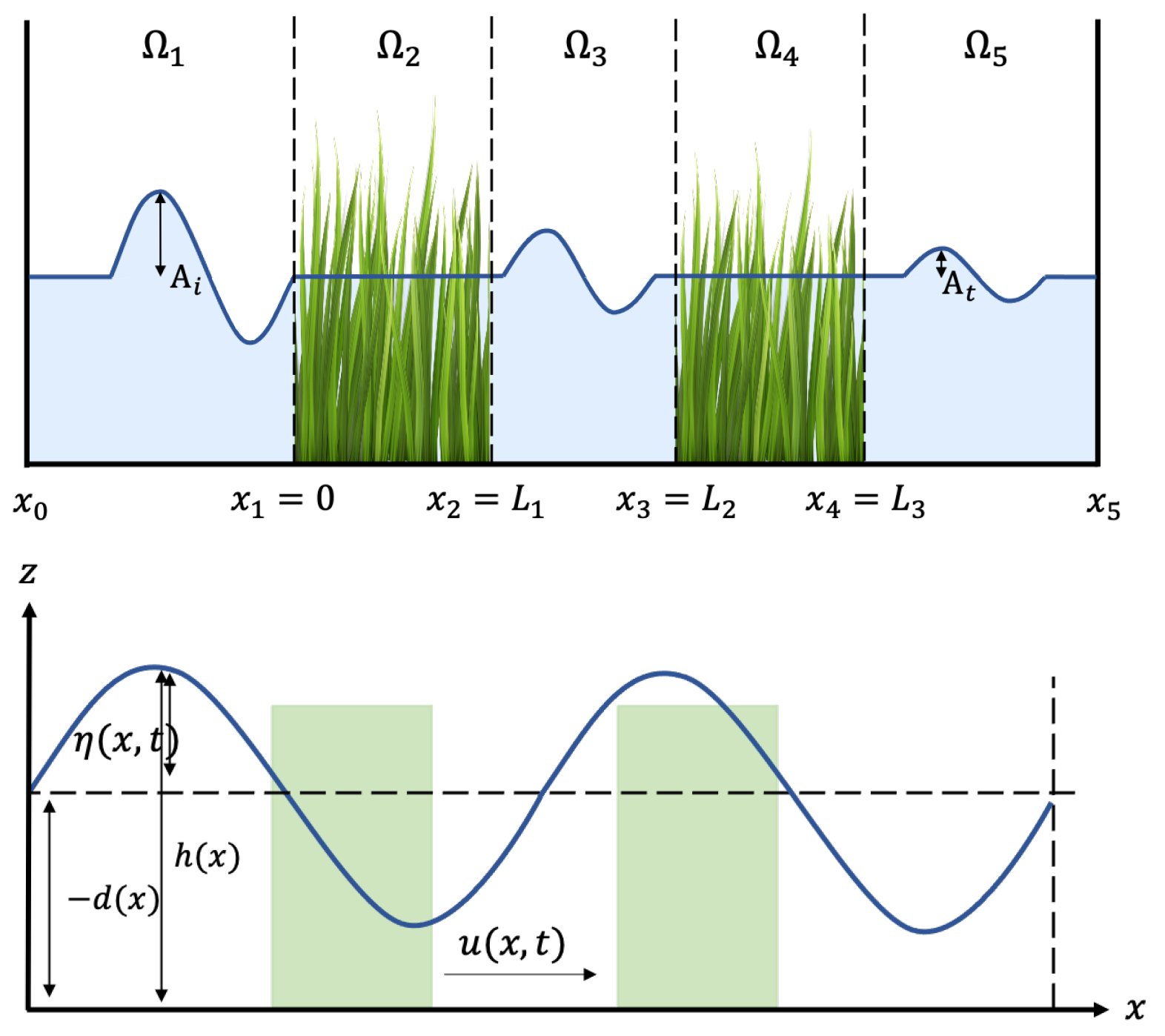
For the 1-D model, we divide the domain of observation into five areas as depicted in Figure 1. The incoming wave enters the observation domain from the left side with the initial amplitude $A_i$ moving towards the right-side with the transmitted amplitude $A_t$. In this 1-D model observation, we consider the bottom profile to be flat, with water depth d. Consider the wave profile for the 1-D model is a function of space x and time t. The SWEs are described as follows.

$${\eta }_t+{\left(hu\right)}_x=0,$$

(1)

$$u_t+g{\eta }_x=0.$$

(2)

In Figure 1, we can see that $d\left(x\right)$ represents the depth of the water and $z=0$ is the still water level. In this observation, the wave enters the domain by a certain period and frequency with the velocity of $u(x,t)$. It will oscillate as far as $\eta (x,t)$ which makes the total water thickness is $h(x,t)=\eta (x,t)+d\left(x\right)$.

Next, we modify the momentum equation to capture the phenomenon. As the wave enters domain ${\Omega }_2$ and ${\Omega }_4$, it will interact with the vegetation, which will cause friction. Therefore, the first modification is the addition of a friction factor, $c_f\omega u$. This particular friction vector is introduced in [54] to allow evaluation of the wave attenuation due to vegetation friction to be performed from knowledge of periodic wave characteristics. The second modification the addition of a diffusion factor. As we know, the diffusion term itself represents damping phenomenon. Therefore, adding a diffusion factor will allow us to capture the attenuation effect caused by the vegetation. Implementing the modifications in the momentum Equation (2) for each domain, we have

$$u_t+g{\eta }_x+c_f\omega u=0,$$

(3)

$$u_t+g{\eta }_x+c_D{u}_{xx}=0,$$

(4)

with piece-wise constant functions of $c_f$ and $c_D$ are described as follow

$$c_f=\left\{\begin{array}{cc}0,& ifx\in {\Omega }_1,{\Omega }_3,{\Omega }_5,\\ f,& ifx\in {\Omega }_2,{\Omega }_4,\end{array}\right.$$

(5)

and

$$c_D=\left\{\begin{array}{cc}0,& ifx\in {\Omega }_1,{\Omega }_3,{\Omega }_5,\\ -D,& ifx\in {\Omega }_2,{\Omega }_4.\end{array}\right.$$

(6)

We use the notation $c_f$ to denote the friction coefficient and $c_D$ to denote the diffusion coefficient, where $\omega$ is the wave frequency and g is the gravitational acceleration.

2.2. Two-Dimensional (2-D) Mathematical Model

In this subsection, we will modify our model even further by constructing the 2-D model. The 2-D model will be beneficial when observing the phenomenon over a real bathymetry profile. For the 2-D model, the observation domain will be divided into three domains ${\Omega }_1,{\Omega }_2,$ and ${\Omega }_3$, with ${\Omega }_2$ is the porous media domain and ${\Omega }_1,{\Omega }_3$ are the non-porous media domains. The 2-D wave profile is a function of the longitudinal distance x, span-wise distance y, and time t. The wave velocity along x-direction is denoted by $u(x,y,t)$ and the wave velocity along y-direction is denoted by $v(x,y,t)$. The initial condition of the velocities are $u(x,y,0)=0$ and $v(x,y,0)=0$, with the initial still water condition is $\eta (x,y,0)=0$. As mentioned before, SWEs are derived from two partial differential equations. Below, Equation (7) represents the mass conservation whereas Equations (8) and (9) are the momentum equations with respect to x and y.

$${\eta }_t+{\left(hu\right)}_x+{\left(hv\right)}_y=0,$$

(7)

$$u_t+g{\eta }_x=0,$$

(8)

$$v_t+g{\eta }_y=0.$$

(9)

As in the case of the 1-D model, Equations (8) and (9) must be modified to capture the phenomenon. Here, we add the same friction and diffusion factor as previously discussed in this paper. Therefore, the governing modified momentum equations for all the three domains are as follows

• Friction term

  $$u_t+g{\eta }_x+c_f\omega u=0,$$

  (10)

  $$v_t+g{\eta }_y+c_f\omega v=0,$$

  (11)

  with

  $$c_f=\left\{\begin{array}{cc}0,& ifx\in {\Omega }_1,{\Omega }_3,\\ f,& ifx\in {\Omega }_2.\end{array}\right.$$

  (12)
• Diffusion term

  $$u_t+g{\eta }_x+c_D{u}_{xx}=0,$$

  (13)

  $$v_t+g{\eta }_y+c_D{v}_{yy}=0,$$

  (14)

  with

  $$c_D=\left\{\begin{array}{cc}0,& ifx\in {\Omega }_1,{\Omega }_3,\\ -D,& ifx\in {\Omega }_2.\end{array}\right.$$

  (15)

3. Analytical Solution

In this section, we will derive the analytical solution for the 1-D SWEs. The analytical solution is in the form of the transmission coefficient $K_t$ which measures the reduction of wave amplitude, hence

$$K_t=\frac{a_t}{a_i}.$$

(16)

Here, $a_i$ refers to the initial amplitude and $a_t$ is the transmitted amplitude. Before we derive the solution for $K_t$, we will construct the solution for $\eta$ and u.

3.1. Solution for $\eta (x,t)$ and $u(x,t)$

First, we derive the solution for $\eta$ and u without the porous media. Recall that we observe the phenomenon in a shallow water environment. Hence, we assume $\eta (x,t)\le d\left(x\right)$ which makes $h(x,t)\approx d\left(x\right)$. In this observation, we also assume $d\left(x\right)$ is a constant through all domains. By implementing these assumptions to Equation (1), we have

$${\eta }_t+d{u}_x=0.$$

(17)

Let $\eta ,u$ be the following functions

$$\eta (x,t)=A\left(x\right)e^{i\omega t},$$

(18)

$$u(x,t)=B\left(x\right)e^{i\omega t}.$$

(19)

Differentiate Equations (18) and (19) with respect to x and t, then substitute the results to the SWEs represented by Equations (2) and (17), we have

$$i\omega A_1\left(x\right)e^{i\omega t}+d{B}_{1x}{e}^{i\omega t}=0,$$

(20)

$$i\omega B_1\left(x\right)e^{i\omega t}+g{A}_{1x}{e}^{i\omega t}=0.$$

(21)

Differentiating Equation (21) over x and substituting it to Equation (20) will give us

$$A_{1xx}+\frac{{\omega }^2}{gd}{A}_1\left(x\right)=0.$$

(22)

By using the method of characteristics, we obtain the solution for Equation (22),

$$A_1\left(x\right)=C_1{e}^{-ikx}+C_2{e}^{ikx},$$

(23)

where $i=\sqrt{(-1)}$, $C_1$ and $C_2$ are undetermined coefficients, and

$$k^2=\frac{{\omega }^2}{gd}.$$

(24)

Next, substituting the derivative of Equation (23) over x to Equation (21) will result in

$$B_1\left(x\right)=\sqrt{\frac{g}{d}}(C_1{e}^{-ikx}-C_2{e}^{ikx}).$$

(25)

Substitute $A_1\left(x\right)$ and $B_1\left(x\right)$, respectively, to Equations (18) and (19), we have the solutions for $\eta$ and u for the domain ${\Omega }_1$ as follow

$${\eta }_1(x,t)=C_1{e}^{-i(kx-\omega t)}+C_2{e}^{i(kx+\omega t)},$$

(26)

$$u_1(x,t)=\sqrt{\frac{g}{d}}(C_1{e}^{-i(kx-\omega t)}-C_2{e}^{i(kx+\omega t)}).$$

(27)

Let $a_i=C_1$ and $a_r=C_2$, where $a_r$ is the reflected amplitude. We have

$${\eta }_1(x,t)=a_i{e}^{-i(kx-\omega t)}+a_r{e}^{i(kx+\omega t)},$$

(28)

$$u_1(x,t)=\sqrt{\frac{g}{d}}(a_i{e}^{-i(kx-\omega t)}-a_r{e}^{i(kx+\omega t)}).$$

(29)

Note that domains ${\Omega }_3$ and ${\Omega }_5$ have the same characteristics as domain ${\Omega }_1$. Therefore, by implementing the exact derivations, we have the solution for $\eta$ and u for domains ${\Omega }_3$ and ${\Omega }_5$ are as follows

$${\eta }_3(x,t)=C_5{e}^{-i(k(x-L_1)-\omega t)}+C_6{e}^{i(k(x-L_1)+\omega t)},$$

(30)

$$u_3(x,t)=\sqrt{\frac{g}{d}}(C_5{e}^{-i(k(x-L_1)-\omega t)}-C_6{e}^{i(k(x-L_1)+\omega t)}),$$

(31)

and

$${\eta }_5(x,t)=C_9{e}^{-i(k(x-L_3)-\omega t)}+C_{10}{e}^{i(k(x-L_3)+\omega t)},$$

(32)

$$u_5(x,t)=\sqrt{\frac{g}{d}}(C_9{e}^{-i(k(x-L_3)-\omega t)}-C_{10}{e}^{i(k(x-L_3)+\omega t)}),$$

(33)

where $C_5,C_6,C_9,$ and $C_{10}$ are undetermined coefficients.

Notice that domain ${\Omega }_5$ is directly connected to the shore and we assume that the wave is absorbed entirely by the shore. This implies that there is no amplitude being reflected from the shore to domain ${\Omega }_5$ which means $a_r=0$. Therefore, if we consider $C_9=a_t$, which is the transmitted amplitude, and $C_{10}=a_r$, then we have

$${\eta }_5(x,t)=a_t{e}^{-i(kx-\omega t)},$$

(34)

$$u_5(x,t)=\sqrt{\frac{g}{d}}(a_t{e}^{-i(kx-\omega t)}).$$

(35)

3.2. Solutions for $\eta (x,t)$ and $u(x,t)$ with Friction Coefficient

In this subsection, we will construct the solutions for $\eta$ and u with porous media represented by friction term. Similarly, by substituting Equations (18) and (19) to the SWEs, we have

$$i\omega A_2\left(x\right)e^{i\omega t}+d{B}_{2x}{e}^{i\omega t}=0,$$

(36)

$$i\omega B_2\left(x\right)e^{i\omega t}+g{A}_{2x}{e}^{i\omega t}+c_f\omega B_2\left(x\right)e^{i\omega t}=0,$$

(37)

then we substitute $B_2\left(x\right)$ from Equation (37) to Equation (36), so that

$$A_{2xx}+\frac{{\omega }^2(1-i{c}_f)}{gd}{A}_2\left(x\right)=0.$$

(38)

By using the same characteristics method and procedures as applied before, the solutions for $A_2\left(x\right)$ and $B_2\left(x\right)$ are

$$A_2\left(x\right)=C_3^{\prime }{e}^{-i{k}_{1}x}+C_4^{\prime }{e}^{i{k}_{1}x},$$

(39)

$$B_2\left(x\right)=\frac{\omega }{k_{1}d}(C_3^{\prime }{e}^{-i{k}_{1}x}-C_4^{\prime }{e}^{i{k}_{1}x}),$$

(40)

where

$$k_1^2=\frac{{\omega }^2(1-i{c}_f)}{gd}.$$

(41)

Therefore, the solutions for domain ${\Omega }_2$ are described as follow

$${\eta }_2(x,t)=C_3^{\prime }{e}^{-i(k_{1}x-\omega t)}+C_4^{\prime }{e}^{i(k_{1}x+\omega t)},$$

(42)

$$u_2(x,t)=\frac{\omega }{k_{1}d}(C_3^{\prime }{e}^{-i(k_{1}x-\omega t)}+C_4^{\prime }{e}^{i(k_{1}x+\omega t)}).$$

(43)

Furthermore, in a similar way, we have the solutions for domain ${\Omega }_4$,

$${\eta }_4(x,t)=C_7^{\prime }{e}^{-i(k_1(x-L_2)-\omega t)}+C_8^{\prime }{e}^{i(k_1(x-L_2)+\omega t)},$$

(44)

$$u_4(x,t)=\frac{\omega }{k_{1}d}(C_7^{\prime }{e}^{-i(k_1(x-L_2)-\omega t)}+C_8^{\prime }{e}^{i(k_1(x-L_2)+\omega t)}).$$

(45)

3.3. Solutions for $\eta (x,t)$ and $u(x,t)$ with Diffusion Coefficient

Similarly, here, we have the solutions for $\eta$ and u with diffusion factor for domain ${\Omega }_2$,

$${\eta }_2(x,t)=C_3{e}^{-i(k_{2}x-\omega t)}+C_4{e}^{i(k_{2}x+\omega t)},$$

(46)

$$u_2(x,t)=\frac{\omega }{k_{2}d}(C_3{e}^{-i(k_{2}x-\omega t)}-C_4{e}^{i(k_{2}x+\omega t)}),$$

(47)

while for domain ${\Omega }_4$,

$${\eta }_4(x,t)=C_7{e}^{-i(k_2(x-L_2)-\omega t)}+C_8{e}^{i(k_2(x-L_2)+\omega t)},$$

(48)

$$u_4(x,t)=\frac{\omega }{k_{2}d}(C_7{e}^{-i(k_2(x-L_2)-\omega t)}-C_8{e}^{i(k_2(x-L_2)+\omega t)}),$$

(49)

where

$$k_2^2=\frac{{\omega }^2}{gd-i\omega c_D}.$$

(50)

In general, the solutions for both $\eta$ and u for each domain are as follow

$$\eta (x,t)=\left\{\begin{array}{cc}{a}_i{e}^{-i(kx-\omega t)}+a_r{e}^{i(kx+\omega t)},& x<0\\ C_3{e}^{-i(k_{j}x-\omega t)}+C_4{e}^{i(k_{j}x+\omega t)},& 0<x<L_1\\ C_5{e}^{-i(k(x-L_1)-\omega t)}+C_6{e}^{i(k(x-L_1)+\omega t)},& L_1<x<L_2\\ C_7{e}^{-i(k_j(x-L_2)-\omega t)}+C_8{e}^{i(k_j(x-L_2)+\omega t)},& L_2<x<L_3\\ a_t{e}^{-i(k(x-L_3)-\omega t)},& x>L_3,\end{array}\right.$$

(51)

$$u(x,t)=\left\{\begin{array}{cc}\sqrt{\frac{g}{d}}(a_i{e}^{-i(kx-\omega t)}-a_r{e}^{i(kx+\omega t)}),& x<0\\ \frac{\omega }{k_{j}d}(C_3{e}^{-i(k_{j}x-\omega t)}-C_4{e}^{i(k_{j}x+\omega t)}),& 0<x<L_1\\ \sqrt{\frac{g}{d}}{e}^{i\omega t}(C_5{e}^{-ik(x-L_1)}-C_6{e}^{ik(x-L_1)}),& L_1<x<L_2\\ \frac{\omega }{k_{j}d}{e}^{i\omega t}(C_7{e}^{-i{k}_j(x-L_2)}-C_8{e}^{i{k}_j(x-L_2)}),& L_2<x<L_3\\ \sqrt{\frac{g}{d}}(a_t{e}^{-i(k(x-L_3)-\omega t)}),& x>L_3,\end{array}\right.$$

(52)

where $j=1,2$ with $k_1^2=\frac{{\omega }^2(1-i{c}_f)}{gd}$ and $k_2^2=\frac{{\omega }^2}{gd-i\omega c_D}$.

Now, we have successfully derived the solutions for $\eta$ and u for each domain. Using this knowledge, we can construct the solution for $K_t$. Notice that in reality, wave elevation and horizontal flux are continuous through all domains. As we can see, both $\eta$ and u have different formula in each domain which is based on whether or not the vegetation is present. Therefore, we must apply ${\eta |}_{x_i^{-}}{=\eta |}_{x_i^{+}}$ and ${u|}_{x_i^{-}}{=u|}_{x_i^{+}}$, where $x_i$ is the discontinue points $0,L_1,L_2,L_3$, for each domain, to maintain wave continuity.

Let $\alpha =1+k/k_j$ and $\beta =1-k/k_j$. By implementing the wave continuity in domain ${\Omega }_1$ and ${\Omega }_2$, we have

$$2a_r=\beta C_3+\alpha C_4,$$

(53)

$$2a_i=\alpha C_3+\beta C_4,$$

(54)

which implies that

$$C_4=\frac{2\alpha a_r-2\beta a_i}{{\alpha }^2-{\beta }^2},$$

(55)

$$C_3=\frac{2\beta a_r-2\alpha a_i}{{\beta }^2-{\alpha }^2}.$$

(56)

Next, for domain ${\Omega }_2$ and ${\Omega }_3$, the results are

$$2C_5=\alpha C_3{e}^{-i{k}_1{L}_1}+\beta C_4{e}^{i{k}_1{L}_1},$$

(57)

$$2C_6=\beta C_3{e}^{-i{k}_1{L}_1}+\alpha C_4{e}^{i{k}_1{L}_1}.$$

(58)

By manipulating Equations (57) and (58), we can express $C_5$ and $C_6$ as follow

$$C_5=\frac{\alpha }{2}\left(\frac{2\beta a_r-2\alpha a_i}{{\beta }^2-{\alpha }^2}\right)e^{-i{k}_j{L}_1}+\frac{\beta }{2}\left(\frac{2\alpha a_r-2\beta a_i}{{\alpha }^2-{\beta }^2}\right)e^{i{k}_j{L}_1},$$

(59)

$$C_6=\frac{\beta }{2}\left(\frac{2\beta a_r-2\alpha a_i}{{\beta }^2-{\alpha }^2}\right)e^{-i{k}_j{L}_1}+\frac{\alpha }{2}\left(\frac{2\alpha a_r-2\beta a_i}{{\alpha }^2-{\beta }^2}\right)e^{i{k}_j{L}_1}.$$

(60)

Moving on to domains ${\Omega }_3$ and ${\Omega }_4$, in a similar way, we yield

$$({\beta }^2-{\alpha }^2)C_8=2\beta C_5{e}^{-ik(L_2-L_1)}-2\alpha C_6{e}^{ik(L_2-L_1)},$$

(61)

$$({\alpha }^2-{\beta }^2)C_7=2\alpha C_5{e}^{-ik(L_2-L_1)}-2\beta C_6{e}^{ik(L_2-L_1)}.$$

(62)

Lastly, for domains ${\Omega }_4$ and ${\Omega }_5$, we have

$$a_t=\frac{k}{k_j}(C_7{e}^{-i{k}_j(L_3-L_2)}-C_8{e}^{i{k}_j(L_3-L_2)}),$$

(63)

$$a_t=C_7{e}^{-i{k}_1(L_3-L_2)}+C_8{e}^{i{k}_1(L_3-L_2)}.$$

(64)

By using all the equations above, we have the final result,

$$K_t=-\frac{4k}{k_j}\frac{({\alpha }^2{\gamma }_4{\gamma }_1-{\beta }^2{\gamma }_2{\gamma }_3)}{{({\alpha }^2-{\beta }^2)}^2({\gamma }_1{\alpha }^2{e}^{i{k}_1(L_3-L_2)}+{\gamma }_3{\beta }^2{e}^{-i{k}_1(L_3-L_2)})},$$

(65)

where

$${\gamma }_1={\beta }^2{e}^{-ik(L_2-L_1)}(e^{-i{k}_j{L}_1}-e^{i{k}_j{L}_1})+e^{ik(L_2-L_1)}({\alpha }^2{e}^{i{k}_j{L}_1}-{\beta }^2{e}^{-i{k}_j{L}_1}),$$

$${\gamma }_2={\alpha }^2{e}^{ik(L_2-L_1)}(e^{i{k}_j{L}_1}-e^{-i{k}_j{L}_1})+e^{-ik(L_2-L_1)}({\alpha }^2{e}^{-i{k}_j{L}_1}-{\beta }^2{e}^{i{k}_j{L}_1}),$$

$${\gamma }_3={\alpha }^2{e}^{-ik(L_2-L_1)}(e^{i{k}_j{L}_1}-e^{-i{k}_j{L}_1})+e^{ik(L_2-L_1)}({\beta }^2{e}^{-i{k}_j{L}_1}-{\alpha }^2{e}^{i{k}_j{L}_1}),$$

$${\gamma }_4={\beta }^2{e}^{ik(L_2-L_1)}(e^{-i{k}_j{L}_1}-e^{i{k}_j{L}_1})-e^{-ik(L_2-L_1)}({\beta }^2{e}^{i{k}_j{L}_1}+{\alpha }^2{e}^{-i{k}_j{L}_1}).$$

We can see that $K_t$ depends on several parameters which are length, friction coefficient $c_f$, and diffusion coefficient $c_D$. The relation between $K_t$ and the parameters will be discussed further in Section 5.

4. Numerical Scheme

In this section, we will discretize our model using the finite volume method on a staggered grid. We will also use an upwind approximation and centered discretization to compute the numerical fluxes. The constructed numerical scheme will be then used for the numerical simulations in Section 5.

4.1. One-Dimension (1-D) Scheme

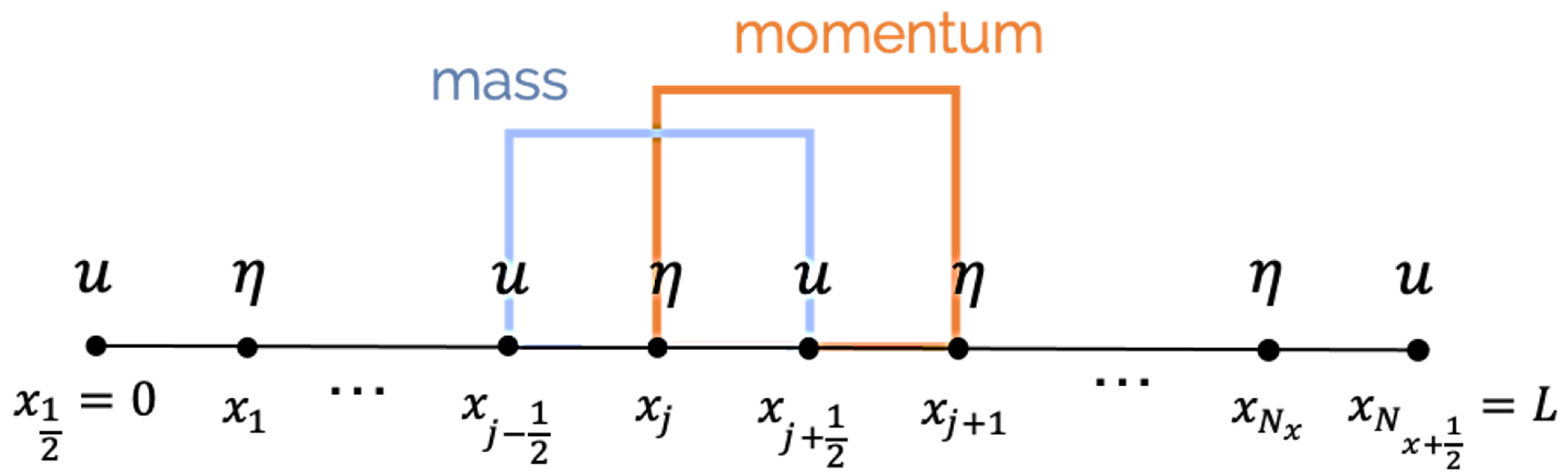
Consider our observation domain to be $\Omega =[0,L]$ and the time interval $t=[0,T]$. The spatial domain is partitioned into $N=\lfloor \frac{L}{\Delta x}\rfloor +1$ cells of the length $\Delta x$ in a staggered way which is $x_{1/2}=0,x_1,\dots ,x_{j-1/2},x_j,x_{j+1/2},\dots ,$ $x_{Nx},x_{Nx+1/2}=L$, as illustrated in Figure 2. Meanwhile, the time interval is divided into $Nt=\lfloor \frac{T}{\Delta t}\rfloor +1$ time steps by the length of $\Delta t$.

In this numerical scheme, we will evaluate the mass conservation Equation (1) in a cell centered at $x_j$ and momentum Equation (2) in cell centered at $x_{j+1/2}$. From this setting, we have the horizontal flow $\eta$ and the water thickness h evaluated in the full grid $x_j$, whereas the wave velocity u is evaluated in the half grid $x_{j+1/2}$. Note that u at the boundary $x=0$ and $x=L$ are always zero. Therefore, by applying the Forward in Time and Center in Space (FTCS) method, we have the following approximations of the 1-D SWEs:

$${\eta }_j^{n+1}={\eta }_j^n-\frac{\Delta t}{\Delta x}(q_{j+1/2}^n-q_{j-1/2}^n),$$

(66)

$$u_{j+1/2}^{n+1}=u_{j+1/2}^n-g\frac{\Delta t}{\Delta x}({\eta }_{j+1}^{n+1}-{\eta }_j^{n+1}),$$

(67)

with $q_{j+1/2}^n{=}^{*}{d}_{j+1/2}^n{u}_{j+1/2}^n,j=1,2,\dots ,N_x$, and $n=1,2,\dots ,N_t$. Here, ${\eta }_j^n$ denotes the approximation of $\eta$ at point $x_j$ and time $t^n$ where $u_{j+1/2}^n$ is the approximation of u at point $x_{j+1/2}$ and time $t^n$. Notice that we evaluate $\eta$ in Equation (67) at $t_{n+1}$ rather than $t_n$. We do this in order to avoid any instability in the scheme. Additionally, according to the Von Neumann stability analysis, the stability condition of numerical scheme (66)–(67) is $0\le \sqrt{g{d}_0}\frac{\Delta t}{\Delta x}\le 1$, with $d_0$ is the flat bottom depth [55,56].

Note that in calculating $q_{j+1/2}^n$, we need the information of $d_{j+1/2}^n$. However, as d shares the same characteristics as h, it is evaluated on the full grid. Thus, we need to approximate the value of d on the half grid, ${}^{*}{d}_{j+1/2}^n$. This is where the upwind approximation will take place. The upwind method will utilize the wave direction to approximate the value of $d_{j+1/2}^n$ as follows

$${}^{*}{d}_{j+1/2}^n=\left\{\begin{array}{cc}{d}_j^n,& u_{j+1/2}\ge 0,\\ d_{j+1}^n,& u_{j+1/2}<0.\end{array}\right.$$

(68)

The upwind approximation works by approximating the value of $d_{j+1/2}$ with the value of d around it. If the wave is moving from left to right, in this case $u_{j+1/2}\ge 0,{\mathrm{then} }^{*}{d}_{j+1/2}^n=d_j^n$, which is the d on its left. This implies that the flux in $x_{j+1/2}$ equals $d_j{u}_{j+1/2}$. The same interpretation applies when the wave is moving towards the left side, $u_{j+1/2}<0$, then ${}^{*}{d}_{j+1/2}^n=d_{j+1}^n$, which is the d on its right. Hence, the flux in $x_{j+1/2}$ equals $d_{j+1}{u}_{j+1/2}$.

Now, as for the modified SWEs, the numerical approximations are as the followings:

• Friction

  $$u_{j+1/2}^{n+1}=\frac{u_{j+1/2}^n-\frac{g\Delta t}{\Delta x}({\eta }_{j+1}^{n+1}-{\eta }_j^{n+1})}{1+\Delta t{c}_f\omega }.$$

  (69)
• Diffusion

  $$u_{j+1/2}^{n+1}=u_{j+1/2}^n-g\frac{\Delta t}{\Delta x}({\eta }_{j+1}^{n+1}-{\eta }_j^{n+1})-c_D\frac{\Delta t}{\Delta x^2}(u_{j+3/2}^n-2u_{j+1/2}^n+u_{j-1/2}^n).$$

  (70)

4.2. Two-Dimension (2-D) Scheme

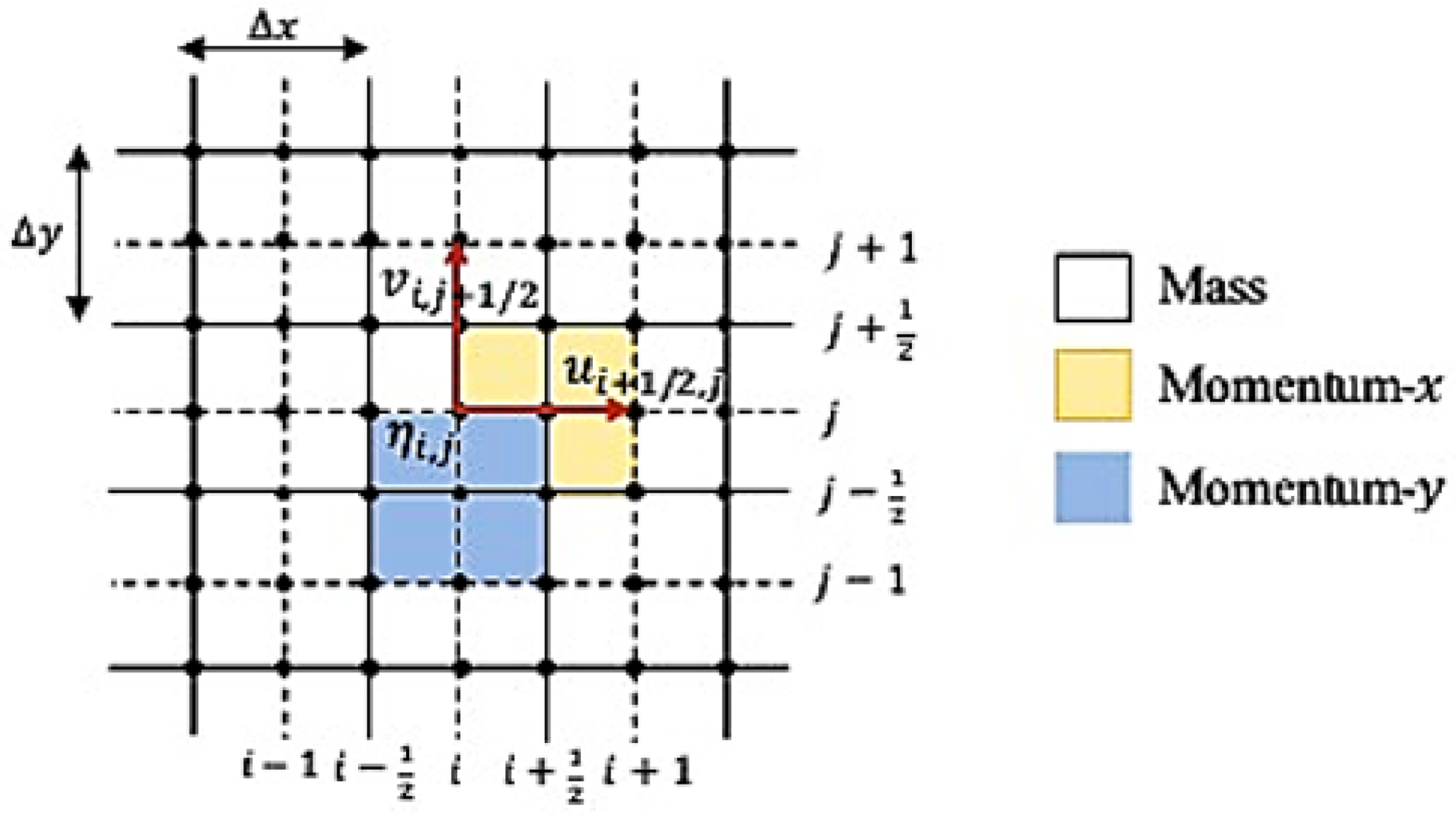
First, we consider the 2-D shallow water equations with the observation domain $\Omega =[0,L_x]{}^{-}[0,L_y]$ and the time interval $t=[0,T]$. The spatial domain is divided using a rectilinear grid of $N_{x^{-}}{N}_y$ and the time interval t is divided into $N_t$ time steps. With the same approach as in the 1-D scheme, we will evaluate $\eta$ and h in the mass conservation equations on the full grid $x_{i,j}$. In contrast, the velocity in the x-direction u and the velocity in y-direction v will be evaluated on the half grid $x_{i-1/2,j}$ and $x_{i,j-1/2}$, respectively, as the Figure 3 shown below.

Here, the indices are $i=1,2,\dots ,N_x$ and $j=1,2,\dots ,N_y$. The approximation of $\eta$ and h at point $x_{i,j}$ and time $t^n$ are represented, respectively, by ${\eta }_{i,j}^n$ and $h_{i,j}^n$. Now, for u, the approximation at point $x_{i+1/2,j}$ and time $t^n$ is denoted by $u_{i+1/2,j}^n$. Meanwhile, at $x_{i,j+1/2}$ and time $t^n$, the approximation of v is denoted by $v_{i,j+1/2}^n$, with $n=1,2,\dots ,N_t$. Consider a scheme at time $t^{n+1}$, the discretization of the 2-D linear SWEs will yield the following equations

$${\eta }_{i,j}^{n+1}={\eta }_{i,j}^n-\frac{\Delta t}{\Delta x}(q_{u(i+1/2,j)}^n-q_{u(i-1/2,j)}^n)-\frac{\Delta t}{\Delta y}(q_{v(i,j+1/2)}^n-q_{v(i,j-1/2)}^n),$$

(71)

$$u_{i+1/2,j}^{n+1}=u_{i+1/2,j}^n-g\frac{\Delta t}{\Delta x}({\eta }_{i+1,j}^{n+1}-{\eta }_{i,j}^{n+1}),$$

(72)

$$v_{i,j+1/2}^{n+1}=v_{i,j+1/2}^n-g\frac{\Delta t}{\Delta y}({\eta }_{i,j+1}^{n+1}-{\eta }_{i,j}^{n+1}),$$

(73)

where $q_{u(i+1/2,j)}^n{=}^{*}{d}_{i+1/2,j}^n{u}_{i+1/2,j}^n$ and $q_{v(i,j+1/2)}^n{=}^{*}{d}_{i,j+1/2}^n{v}_{i,i+1/2}^n$. The Von Neumann stability analysis for the 2-D linear SWEs provides the stability condition for Equations (71)–(73), which is $0\le \Delta t\sqrt{g{d}_0}(\frac{1}{\Delta x^2}+\frac{1}{\Delta y^2})\le 1$ [57].

Next, we need to approximate the value of d on the half grid $x_{i+1/2,j}$ and $x_{i,j+1/2}$. Similarly, using the upwind approximation for all $(i,j)\in \{1,...,N_x\}\times \{1,...,N_y\}$, we have

$${}^{*}{d}_{i+1/2,j}^n=\left\{\begin{array}{cc}{d}_{i,j}^n,& u_{i+1/2,j}\ge 0,\\ d_{i+1,j}^n,& u_{i+1/2,j}<0,\end{array}\right.$$

(74)

$${}^{*}{d}_{i,j+1/2}^n=\left\{\begin{array}{cc}{d}_{i,j}^n,& v_{i,j+1/2}\ge 0,\\ d_{i,j+1}^n,& v_{i,j+1/2}<0.\end{array}\right.$$

(75)

For the vertical components, when the flow is moving up, $v_{i,j+1/2}^n\ge 0$, we use the information from below, which is $d_{i,j}$. However, if the flow is moving towards the bottom, $v_{i,j+1/2}^n<0$, then the information of the upper flow, $d_{i,j+1}$, is used. For the horizontal components, we treat them as described in the 1-D scheme.

As for the modified momentum equations, the discretizations are as follows:

• Friction

  $$u_{i+1/2,j}^{n+1}=\frac{u_{i+1/2,j}^n-g\frac{\Delta t}{\Delta x}({\eta }_{i+1,j}^{n+1}-{\eta }_{i,j}^{n+1})}{1+\Delta t{c}_f\omega },$$

  (76)

  $$v_{i,j+1/2}^{n+1}=\frac{v_{i,j+1/2}^n-g\frac{\Delta t}{\Delta y}({\eta }_{i,j+1}^{n+1}-{\eta }_{i,j}^{n+1})}{1+\Delta t{c}_f\omega }.$$

  (77)
• Diffusion

$$u_{i+1/2,j}^{n+1}=u_{i+1/2,j}^n-g\frac{\Delta t}{\Delta x}({\eta }_{i+1,j}^{n+1}-{\eta }_{i,j}^{n+1})-c_D\frac{\Delta t}{\Delta x^2}(u_{i+3/2,j}^n-2u_{i+1/2,j}^n+u_{i-1/2,j}^n),$$

(78)

$$v_{i,j+1/2}^{n+1}=v_{i,j+1/2}^n-g\frac{\Delta t}{\Delta y}({\eta }_{i,j+1}^{n+1}-{\eta }_{i,j}^{n+1})-c_D\frac{\Delta t}{\Delta y^2}(v_{i,j+3/2}^n-2u_{i,j+1/2}^n+u_{i,j-1/2}^n).$$

(79)

5. Numerical Simulation and Discussion

Here, we will implement our numerical schemes to simulate the wave propagation phenomena for both the 1-D and 2-D models. The simulations will allow us to observe how porous media affects wave amplitude. Furthermore, we will compare the results with those from an experiment and those of the analytical solutions. For the simulations in this research, all parameters, including the axes in the figures, are in SI units.

5.1. One-Dimension (1-D) Numerical Simulations

For the 1-D simulation, we choose $0<x<L$ as the spatial domain, with $L=30$ and water thickness $d=10$, along all x. The porous media will be placed in domains ${\Omega }_2$ and ${\Omega }_4$, where ${\Omega }_2=\left\{x\right|5<x<10\}$ and ${\Omega }_4=\left\{x\right|15<x<20\}$. We consider an incoming monochromatic sinusoidal wave, which enters the observation domain from the left side moving towards the right side. We choose the initial conditions to be the following:

$$\eta (x,0)=0,$$

(80)

$$u(x,0)=0.$$

(81)

For the left boundary condition, we take a monochromatic sinusoidal wave with the initial amplitude $A=0.1$ m and wave frequency $\omega =2\pi$,

$$\eta (0,t)=Asin\left(\omega t\right),$$

(82)

and as for the right boundary, we apply the absorbing boundary condition, with $g=9.81$, as follows

$$u(L,t)=\sqrt{\frac{g}{h}}\eta (L,t).$$

(83)

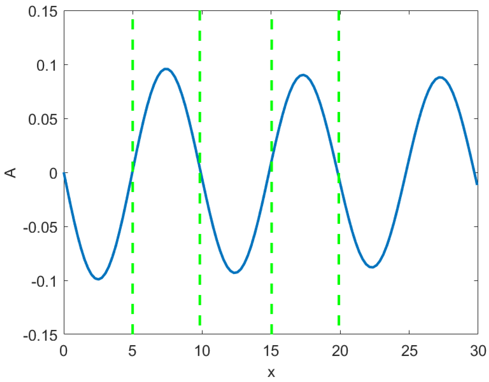
First, we will simulate the wave propagation phenomenon with the friction coefficient. We choose the friction coefficient $c_f=0.32$, the spatial partition $\Delta x=0.2$, and the time partition $\Delta t=\frac{\Delta x}{\sqrt{gd}}$, in order to maintain stability. The result of the 1-D numerical simulation is presented below. The green areas represent the vegetation (porous media) and the blue line represents the surface wave elevation.

From Figure 4, we can see that the wave amplitude is reduced after passing through the vegetation. The reduction of the wave amplitude can be seen more clearly with the numerical transmission coefficient $K_t$ computed from the simulation. The numerical simulation gives us the result of $K_t=0.3767$. This tells us that the porous media reduces the wave amplitude by more than $60\%$ of the initial amplitude.

Now, for the diffusion factor, we set the diffusion coefficient, the spatial partition, and the time partition as $c_D=0.6,\Delta x=0.23$, and $\Delta t=0.01$, respectively. In Figure 5, we can see the outcome of the 1-D numerical simulation.

Notice that after passing through the porous media, there is a slight decrease in the wave amplitude. The numerical simulation gives us the result of the transmission coefficient $K_t=0.8166$. From both results, we can conclude that both models, with friction and diffusion coefficient, have successfully captured the phenomenon of wave reduction caused by the porous media. However, the reduction caused by friction is more significant than diffusion.

In addition, for this 1-D model, we have performed a simulation to evaluate the computational cost of our model and its comparison against an existing model, which is a Boussinesq-type model. Since we are not studying the Boussinesq-type model for wave-vegetation interaction cases, in this comparison, we only simulate the more simple wave phenomenon, which is standing wave. In the simulations, we use a spatial domain of $[0,250]$ with observation time of $T=15$. All the parameters, including $\Delta x$, $\Delta t$, gravity acceleration, and water depth are set to be exactly the same. After simulating both models, it was found that the computational cost for Boussinesq-type model is about $0.651996$ s. Meanwhile, our SWEs give a computational cost of around $0.075074$ s, which is almost 10 times smaller than Boussinesq-type model’s. This finding confirms that our model is much less expensive than another existing model, in this case, Boussinesq-type model.

5.2. Comparing the One-Dimensional (1-D) Numerical and Analytical Result

In this subsection, we will compare the numerical and analytical values of transmission coefficient $K_t$. The numerical $K_t$ is computed in the same way as the analytical $K_t$. We compute the numerical $K_t$ by comparing the maximum value of $\eta$ in domain ${\Omega }_5$ with the maximum value of $\eta$ in domain ${\Omega }_1$. We will compute $K_t$ with different parameters of the porous media. This will help us to understand more about the relationship between the porous media and wave amplitude reduction.

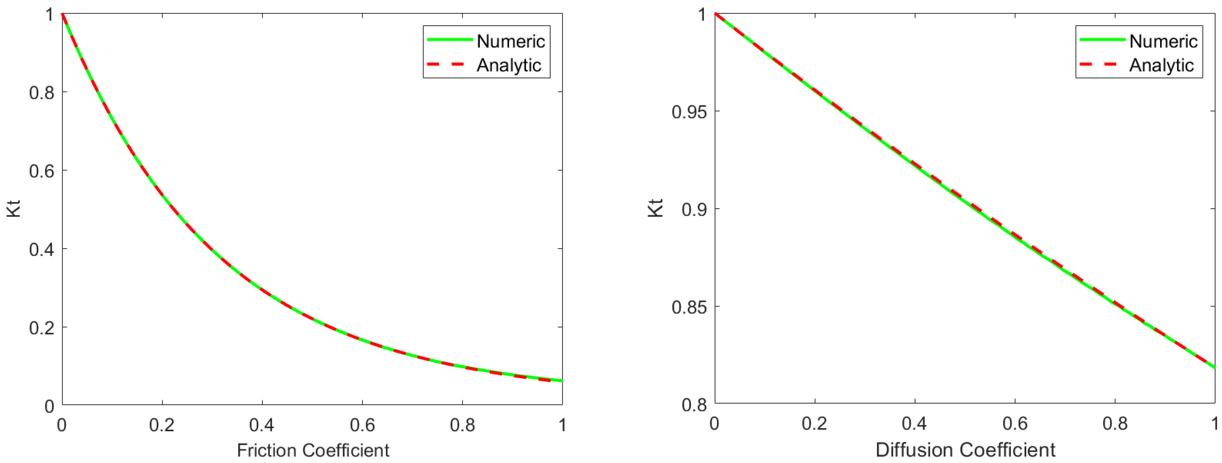
First, we will conduct several numerical simulations using different $c_f$ and $c_D$. The observation domain is $\Omega =\left\{x\right|0<x<20\}$, the water depth is $H=10$, the porous media is located in ${\Omega }_2=\left\{x\right|5<x<10\}$ and ${\Omega }_4=\left\{x\right|15<x<20\}$, while the spatial partition is $\Delta x=0.1$. The incoming wave is set to be $\eta (0,t)=Asin\left(\omega t\right)$, with the amplitude $A=0.1,\omega =2\pi$, and time $T=7$.

The results from the numerical simulations approximate our analytical solutions well when describing the relation between $K_t$ with both $c_f$ and $c_D$, as depicted in Figure 6. After several simulations, we obtain that the RMSE of the numerical approximations towards the analytical solutions is $3.7\times {10}^{-5}$ for friction and $0.874$ for diffusion.

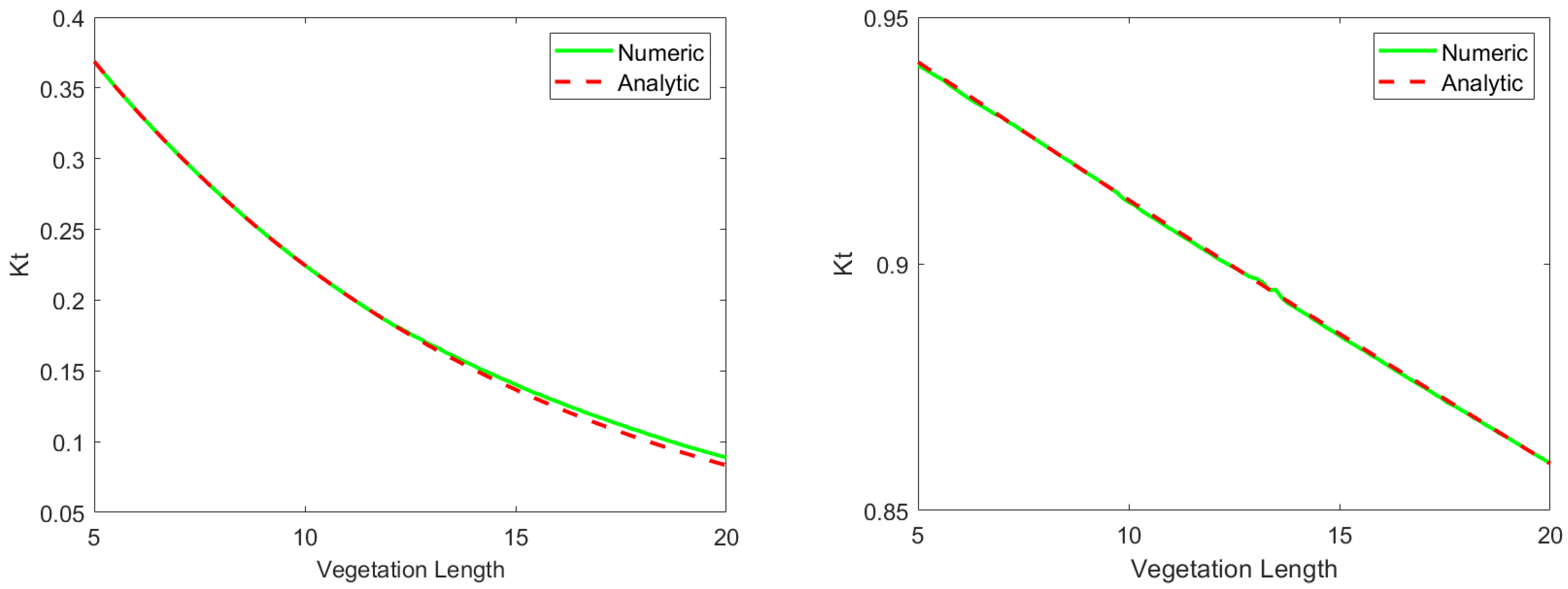
We also compare the numerical and analytical solutions of the relation between transmission coefficient $K_t$ and the vegetation length. We conduct multiple simulations using different vegetation lengths. Similar to the analytical solutions, the numerical solutions give us the result that the relation between the transmission coefficient $K_t$ and the length of vegetation is significant. From Figure 7, we can see that the discrepancy between the numerical and analytical transmission coefficient $K_t$ is hardly noticeable. This implies that our numerical solutions successfully approximate the analytical solutions with the RMSE of $1.8\times {10}^{-4}$ for phenomenon with friction factor and $0.852$ with diffusion. From Figure 6 and Figure 7, we can conclude that $K_t$ has a strong relation with $c_f,c_D$, and the length of vegetation. The transmission coefficient will gradually decrease along with the increase of these parameters.

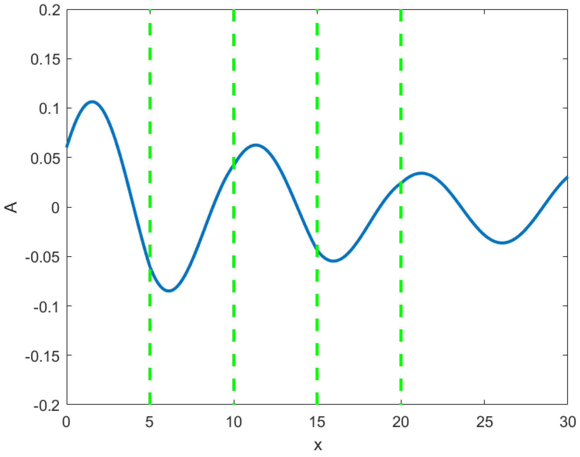
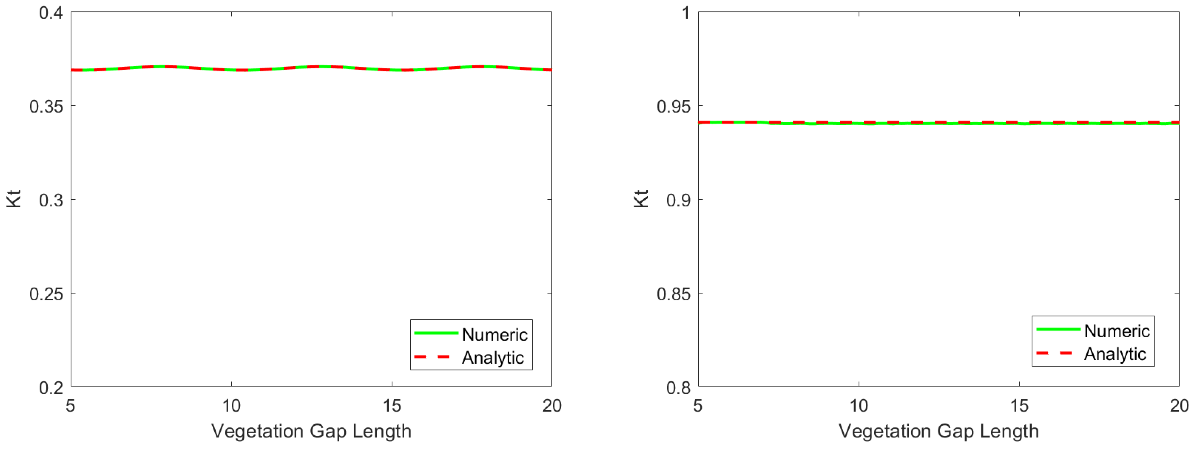
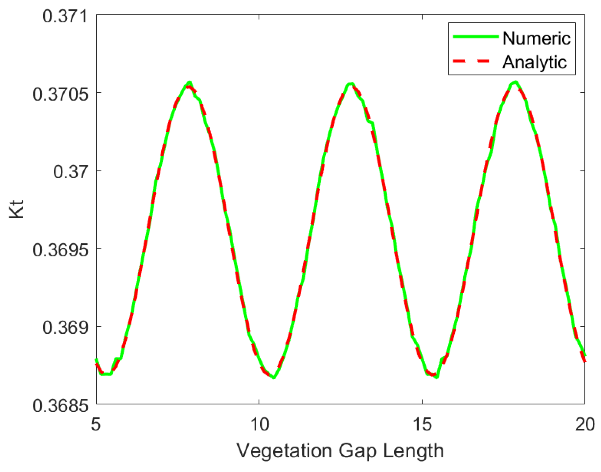
Next, from Figure 8, we can see that $K_t$ remains almost constant throughout the changes of vegetation distance. If we take a closer look to the Figure 8, we will see that transmission coefficient $K_t$ does oscillate over different vegetation distances. The numerical simulation using friction coefficient $c_f$ gives us a clear representation of this phenomenon, as depicted in Figure 9. From these results, we can say that the distance between vegetation patches do not have a significant effect upon $K_t$. The numerical solutions approximate the analytical solutions with RMSE of $2.1\times {10}^{-5}$ for friction, whereas for diffusion, the RMSE is $0.765$.

We can conclude that the transmission coefficient and the distance of the vegetation do not have a particular relation. In other words, the distance between vegetation is insignificant towards the reduction of wave amplitude by the porous media. The results of the numerical approximations towards the analytical solutions are very satisfactory with the RMSE value close to zero. This implies that our numerical scheme is validated, since it successfully approximates our analytical solutions.

5.3. Two-Dimensional (2-D) Numerical Simulations

The 2-D numerical simulation will help us investigate and understand more about the effectiveness of the porous media on the reduction of wave amplitude over an uneven bottom. We have conducted an experiment in Demak and now will compare the experiment results with the numerical results.

Consider a monochromatic wave with period T, which enters the observation domain $\Omega =\left\{(x,y,t)\right|0<x<L_x,0<y<L_y,t<T_{observation}\}$, with the spatial partition $\Delta x$, $\Delta y$, and the time partition $\Delta t$. The initial conditions for the 2-D numerical simulation are as follows:

$$\eta (x,y,0)=0,$$

(84)

$$u(x,y,0)=0,$$

(85)

$$v(x,y,0)=0.$$

(86)

Similar to the 1-D numerical simulations, for the left boundaries, we use

$$\eta (0,y,t)=Asin\left(\omega t\right).$$

(87)

In this 2-D numerical simulation, we are going to stop the simulation before the wave reaches the dry area to avoid any instability. Therefore, any right boundary for this simulation is applicable.

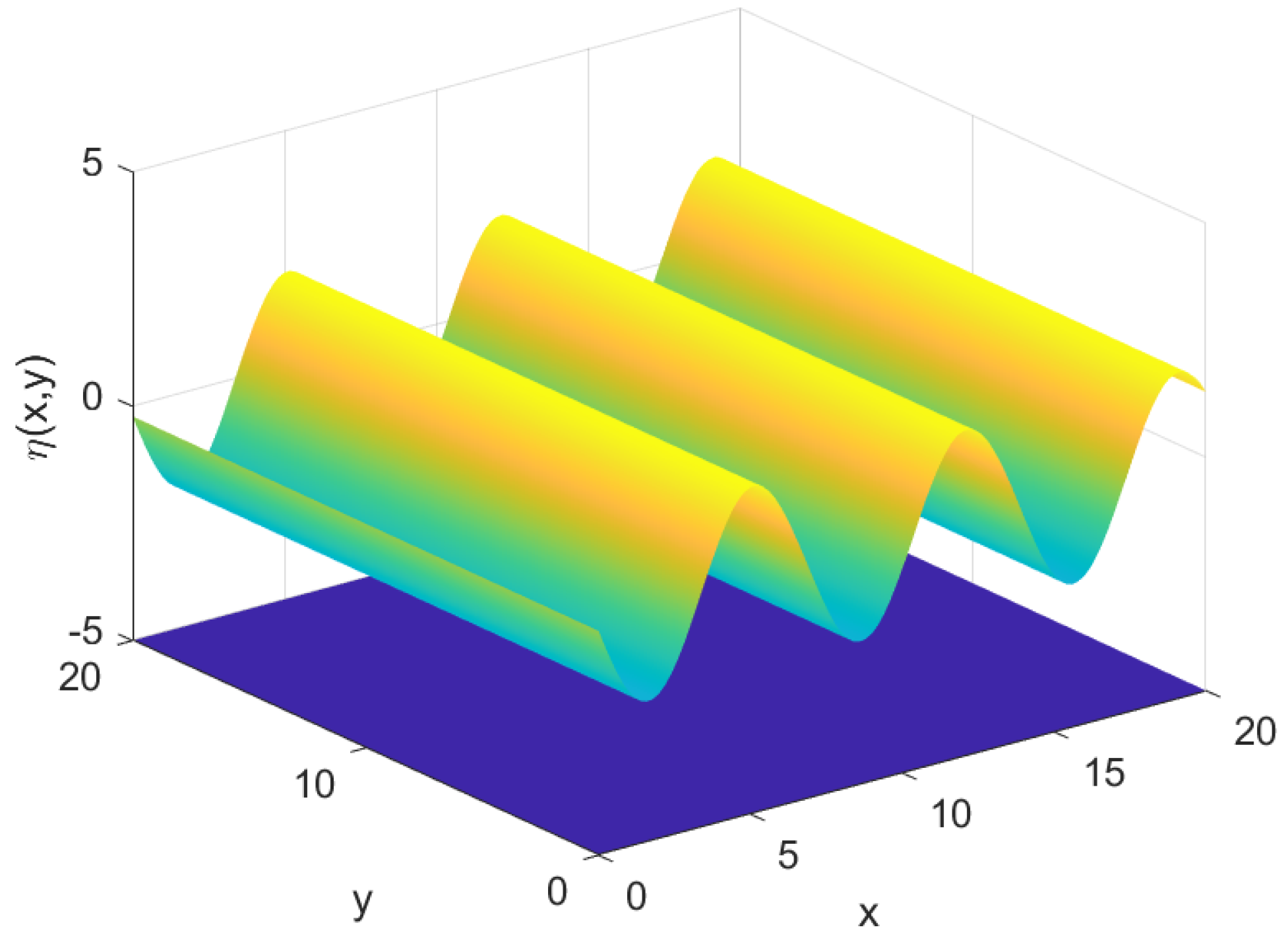
First, we simulate our 2-D scheme over a flat bottom. This is to make sure that our scheme is stable for the entire 2-D simulation. We will simulate a monochromatic sinusoidal wave entering the observation domain. The observation domain is set to be $\Omega =\left\{(x,y,t)\right|0<x<40,0<y<50,t<7\},\Delta x=0.2,\Delta y=0.2,\Delta t=\frac{\Delta x}{\sqrt{gd}}$, with $g=9.81$ and $d=5$.

We consider an incoming wave $\eta (0,y,t)=Asin\left(2.5t\right)$ and $A=1$ is the wave amplitude. Figure 10 gives us the result of the simulation. Notice that the waveform and amplitude remain the same throughout the entire simulation. Therefore, we can conclude that our 2-D model works perfectly in this setting.

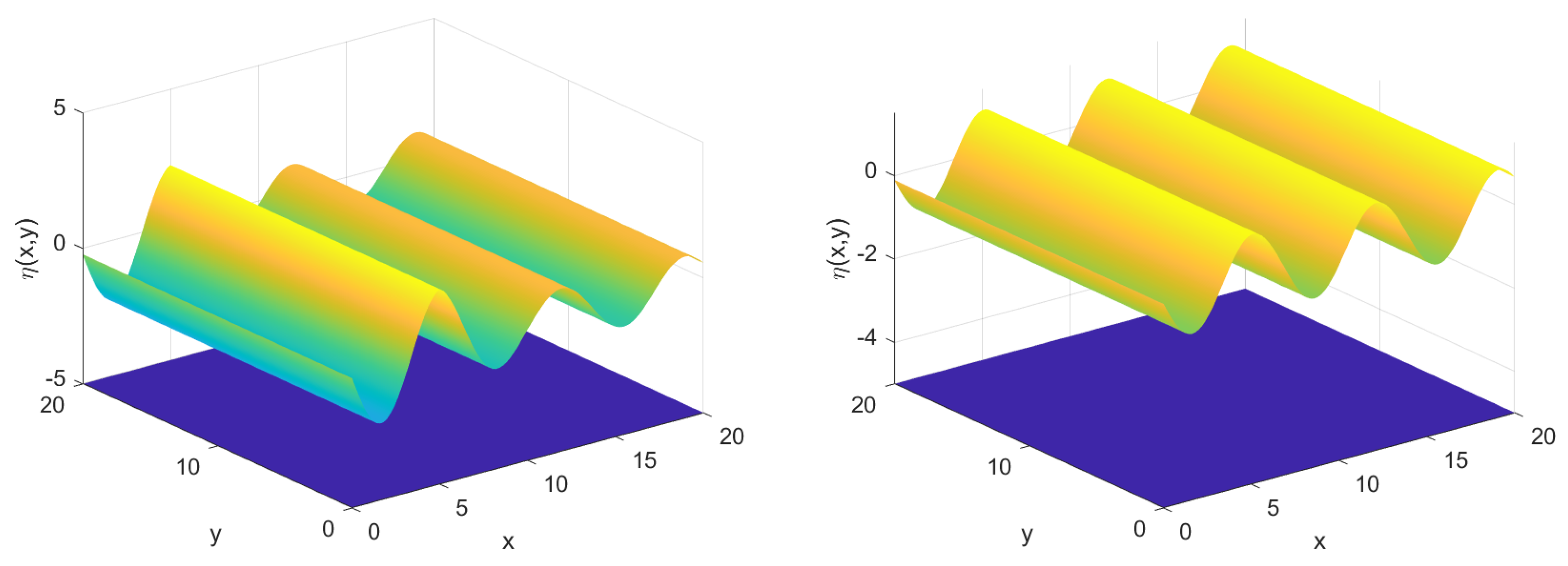
Next, we will simulate the wave propagation phenomenon over a flat bottom profile by adding porous media to our simulation. We are going to implement Equations (76)–(79) with the settings of $\Omega =\left\{(x,y,t)\right|0<x<20,0<y<20,t<5\},\Delta x=0.2,\Delta y=0.2,\Delta t=\frac{\Delta x}{\sqrt{gd}},g=9.81$, and $d=5$. The porous media will take place in ${\Omega }_2=\left\{(x,y)\right|5<x<10,0<y<50\}$, with $c_f=0.32$ and $c_D=0.15$. Consider a monochromatic sinusoidal wave $\eta (0,y,t)=Asin\left(\omega t\right)t$, with $A=1$ and $\omega =2\pi$, which enters the observation domain. We have the results of the numerical simulations as follows.

From Figure 11, we can see that the addition of the porous media, which represented by the green area, causes the wave amplitude to decrease. The result of the simulation with friction captures this phenomenon perfectly, whereas for diffusion, it is slightly harder to observe in plain view. Another way to observe the reduction is by calculating the transmission coefficient. The numerical transmission coefficient $K_t$ computed by our simulation gives us the result of $K_t=0.4966$ for friction and $K_t=0.9574$ for diffusion.

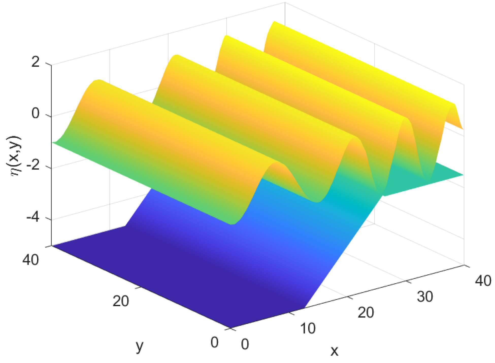
Next, we continue to conduct numerical simulation using a real bathymetry profile. In this simulation, the wave will move from the deeper water level towards the shallower water area. The change in water depth will cause some of the wave properties such as length, height, and velocity to change. This phenomenon is called wave shoaling. The interpretation of this phenomenon can be seen in Figure 12, using an artificial bottom profile.

As we can see in Figure 12, the wave amplitude increases as the wave approaches the shallow water level. Therefore, in order to measure the wave amplitude reduction by the porous media, we cannot use transmission coefficient $K_t$ alone. We need to compare the $K_t$ with the shoaling coefficient $K_s$. $K_s$ measures the ratio of wave heights in two different water levels. The difference between $K_s$ and $K_t$ is that $K_s$ is calculated without any interference of the porous media. We are going to use the analytical shoaling coefficient as stated in [57], which is described as the following,

$$K_s=\frac{H_2}{H_1}=(\frac{\sqrt{g{d}_1}}{\sqrt{g{d}_2}})(\frac{1}{2})=(\frac{d_1}{d_2})(\frac{1}{4}),$$

(88)

where $H_1$ represents the initial wave amplitude at water depth $d_1$, whereas $H_2$ represents the wave amplitude in shallow water level $d_2$.

For the simulation using a real bathymetry profile, we set the domain to be $\Omega =\left\{(x,y,t)\right|0<x<50,0<y<50,0<t<2\},\Delta x=0.25,\Delta y=0.25,\Delta t=\frac{\Delta x}{\sqrt{gd}},g=9.81$. We place the porous media in ${\Omega }_2=\left\{(x,y)\right|5<x<15,0<y<50\}$, the initial wave is $\eta (0,y,t)=Asin\left(15t\right)t$, and the initial amplitude is $A=10$.

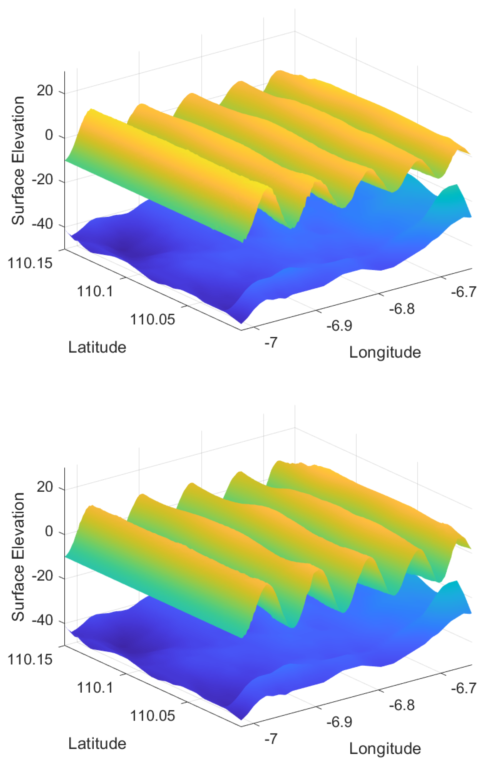
Figure 13 gives us the results of the 2D numerical simulations of wave propagation phenomenon with friction and diffusion coefficient. The wave amplitude reduction was not captured clearly in Figure 13. We can still observe how the porous media reduces the wave amplitude through transmission coefficient $K_t$. The numerical simulation gives us the result of shoaling coefficient $K_s=1.0552$ and friction $K_t=0.5148$, whereas diffusion $K_t=0.8184$. This implies that the porous media reduces the wave amplitude by more than $50\%$ using friction and $23\%$ using diffusion. Therefore, our 2-D numerical model successfully captured the wave amplitude reduction caused by the porous media.

5.4. Comparing the Two-Dimensional (2-D) Numerical Result and Real Experiment Data

Here, we will compare the numerical simulation results with real experiment data. The experiment took place in Demak on 6–7 February 2020. In simulating our numerical solution, we will use the 2-D model and real bathymetry profile of Demak as depicted in Figure 13. We retrieved the bathymetry data from GEBCO with longitude of $[-6.5205-7.0205]$ and latitude of $\left[110.0058110.3059\right]$.

For the numerical simulation with friction factor, we will set the spatial partition to be $\Delta x=\Delta y=0.3$ and $c_f=0.2$. Whereas for diffusion, $\Delta x=\Delta y=0.5$ and $c_D=1$. The friction factor $c_f$ and diffusion factor $c_d$ applied in the two dimensional (2-D) mathematical model are based on the range of $c_f$ and $c_d$ implied in the one dimensional (1-D) mathematical model which gave the minimum error. Furthermore, we iterate $c_f$ and $c_d$ within the given range to fit our actual experiment data in order to achieve the minimum error. The results of both experiment and numerical simulations are shown in

Table 1. Comparison between the Transmission Coefficient $K_t$ obtained using Experimental and Numerical approach.

Date	Time	Water Height		${\mathit{K}}_{\mathit{t}}$ Experimental	${\mathit{K}}_{\mathit{t}}$ Numerical		Error (%)
		Land-Ward	Sea-Ward		Friction	Diffusion	Friction	Diffusion
6 Feb	18.00	63	97	0.65	0.64	0.68	2	4
	18.30	66	100	0.66	0.64	0.68	3	2
	19.00	60	92	0.65	0.64	0.68	2	4
	19.30	58	89	0.65	0.64	0.68	2	4
7 Feb	18.30	91	142	0.64	0.64	0.68	0	5
	19.00	43	69	0.62	0.64	0.68	2	8
	19.30	50	75	0.67	0.64	0.68	4	1
	20.00	57	86	0.66	0.64	0.68	4	2

.

As we can see in Table 1, our numerical $K_t$ approximates the experimental $K_t$ well with errors of less than $10\%$ for both friction and diffusion model. This implies that our 2-D numerical scheme successfully captures the phenomenon and estimates wave attenuation by vegetation over a real bathymetry. Thus, we can say that our model is quite applicable to be used in real coastal areas. Therefore, it can be used to design an effective porous media in the form of vegetation as an actual coastal protection against wave attack. Further, from Table 1, we also can conclude that, in this specific case, the presence of vegetation can help reduce the wave amplitude by more than $30\%$.

In addition, We have also calculated the computational cost of our model for this particular case. The results are different for friction and diffusion model. For model involving friction coefficient, the computational cost is found to be $4.573120$ s, while for model with diffusion term, the computational cost is $2.375985$ s. Despite the fact that the first model gives a computational cost twice as expensive as the second one, but fairly, both models can be executed in a quite short of time. This finding, supported by the comparison of the computational cost between 1-D SWEs and 1-D Boussinesq-type model mentioned previously, can be used to confirm that our model is indeed less expensive than other previous model, especially Boussinesq-type model.

6. Conclusions

From this research, we successfully captured and described the wave attenuation by vegetation phenomenon through the wave transmission coefficient $K_t$ from both the analytical and numerical solutions. Moreover, the numerical scheme is validated by the results from the analytical solutions and real experimental data with the relative error below $10\%$. Through numerous simulations, we can conclude that the wave attenuation factors are friction coefficient $c_f$, diffusion coefficient $c_D$, and vegetation length. These three properties of the porous media profoundly affect $K_t$. If just one of these coefficients increases, then $K_t$ will decrease, therefore, increasing the wave attenuation significantly. Furthermore, there are two additional interesting findings from this research. First, the proportion of $K_t$ reduction caused by the increase of $c_f$ is much higher than $c_D$, which implies that the friction factor affects wave attenuation more than the diffusion factor. Second, the length between vegetation patches does not have a particular effect on $K_t$, which means that the distance between vegetation is relatively insignificant compared to other parameters. All in all, this research can be used as an evaluation tool to determine coastal protection using porous media, specifically mangroves.

References

- Kopp, R.E.; Horton, R.M.; Little, C.M.; Mitrovica, J.X.; Oppenheimer, M.; Rasmussen, D.J.; Strauss, B.H.; Tebaldi, C. Probabilistic 21st and 22nd century sea-level projections at a global network of tide-gauge sites. Earth’s Future 2014, 2, 383–406. [Google Scholar] [CrossRef]
- Kopp, R.E.; DeConto, R.M.; Bader, D.A.; Hay, C.C.; Horton, R.M.; Kulp, S.; Oppenheimer, M.; Pollard, D.; Strauss, B.H. Evolving Understanding of Antarctic Ice-Sheet Physics and Ambiguity in Probabilistic Sea-Level Projections. Earth’s Future 2017, 5, 1217–1233. [Google Scholar] [CrossRef] [Green Version]
- Nauels, A.; Meinshausen, M.; Mengel, M.; Lorbacher, K.; Wigley, T.M.L. Synthesizing long-term sea level rise projections the MAGICC sea level model v2.0. Geosci. Model Dev. 2017, 10, 2495–2524. [Google Scholar] [CrossRef] [Green Version]
- Nauels, A.; Rogelj, J.; Schleussner, C.F.; Meinshausen, M.; Mengel, M. Linking sea level rise and socioeconomic indicators under the Shared Socioeconomic Pathways. Environ. Res. Lett. 2017, 12, 114002. [Google Scholar] [CrossRef] [Green Version]
- Bakker, A.M.R.; Wong, T.E.; Ruckert, K.L.; Keller, K. Sea-level projections representing the deeply uncertain contribution of the West Antarctic ice sheet. Sci. Rep. 2017, 7. [Google Scholar] [CrossRef] [Green Version]
- Wong, T.E.; Bakker, A.M.; Keller, K. Impacts of Antarctic fast dynamics on sea-level projections and coastal flood defense. Clim. Chang. 2017, 144, 347–364. [Google Scholar] [CrossRef]
- Jevrejeva, S.; Moore, J.; Grinsted, A. Sea level projections to AD2500 with a new generation of climate change scenarios. Glob. Planet. Chang. 2012, 80, 14–20. [Google Scholar] [CrossRef]
- Altomare, C.; Crespo, A.; Rogers, B.D.; DomÃnguez, J.M.; Gironella, X.; Gesteira, M. Numerical Modelling of Armour Block Sea Breakwater with Smoothed Particle Hydrodynamics. Comput. Struct. 2014, 130, 34–45. [Google Scholar] [CrossRef]
- Johnson, H. Wave modelling in the vicinity of submerged breakwaters. Coast. Eng. 2006, 53, 39–48. [Google Scholar] [CrossRef]
- Balaji, R.; Kumar, S.S.; Misra, A. Understanding the effects of seawall construction using a combination of analytical modelling and remote sensing techniques: Case study of Fansa, Gujarat, India. Int. J. Ocean Clim. Syst. 2017, 8, 153–160. [Google Scholar] [CrossRef] [Green Version]
- Magdalena, I.; Atras, M.F.; Sembiring, L.; Nugroho, M.A.; Labay, R.S.B.; Roque, M.P. Wave Transmission by Rectangular Submerged Breakwaters. Computation 2020, 8, 56–73. [Google Scholar] [CrossRef]
- Magdalena, I.; Iryanto; Reeve, D. Free-surface long wave propagation over linear and parabolic transition shelves. Water Sci. Eng. 2018, 11, 318–327. [Google Scholar] [CrossRef]
- Pudjaprasetya, S.R.; Magdalena, I. Wave Energy Dissipation over Porous Media. Appl. Math. Sci. 2013, 7, 2925–2937. [Google Scholar] [CrossRef]
- Ondiviela, B.; Losada, I.; Lara, J.; Maza, M.; Galvan, C.; Bouma, T.; Belzen, J. The Role of Seagrass in Coastal Protection in a Changing Climate. J. Coast. Eng. 2013, 87, 158–168. [Google Scholar] [CrossRef]
- Borsje, B.W.; van Wesenbeeck, B.K.; Dekker, F.; Paalvast, P.; Bouma, T.J.; van Katwijk, M.M.; de Vries, M.B. How ecological engineering can serve in coastal protection. Ecol. Eng. 2011, 37, 113–122. [Google Scholar] [CrossRef]
- Vuik, V.; Jonkman, S.N.; Borsje, B.W.; Suzuki, T. Nature-based flood protection: The efficiency of vegetated foreshores for reducing wave loads on coastal dikes. Coast. Eng. 2016, 116, 42–56. [Google Scholar] [CrossRef] [Green Version]
- deVriend, H.J.; van Koningsveld, M.; Aarninkhof, S.G.J.; de Vries, M.B.; Baptist, M.J. Sustainable hydraulic engineering through building with nature. J. Hydro-Environ. Res. 2015, 9, 159–171. [Google Scholar] [CrossRef]
- Temmerman, S.; Meire, P.; Bouma, T.J.; Herman, P.M.J.; Ysebaert, T.; de Vriend, H. Ecosystem-based coastal defence in the face of global change. Nature 2013, 504, 79–83. [Google Scholar] [CrossRef] [PubMed]
- Cuc, N.T.K.; Suzuki, T.; van Steveninck, E.D.R.; Hai, H. Modelling the impacts of mangrove vegetation structure on wave dissipation in Ben Tre Province, Vietnam, under different climate change scenarios. J. Coast. Res. 2015, 31, 340–347. [Google Scholar] [CrossRef] [Green Version]
- Hu, Z.; Suzuki, T.; Zitman, T.; Uittewaal, W.; Stive, M. Laboratory study on wave dissipation by vegetation in combined current-wave flow. Coast. Eng. 2014, 88, 131–142. [Google Scholar] [CrossRef]
- Chen, H.; Ni, Y.; Li, Y.; Liu, F.; Ou, S.; Su, M.; Peng, Y.; Hu, Z.; Wim, U.; Tomohiro, S. Deriving vegetation drag coefficients in combined wave-current flows by calibration and direct measurement methods. Adv. Water Resour. 2018, 122, 217–227. [Google Scholar] [CrossRef] [Green Version]
- Hasselmann, K.; Collins, J.I. Spectral dissipation of finite-depth gravity waves due to turbulent bottom friction. J. Mar. Res. 1968, 26, 1–12. [Google Scholar]
- Möller, I.; Spencer, T.; French, J.R.; Leggett, D.J.; Dixon, M. Wave transformation over salt marshes: A field and numerical modelling study from north Norfolk, England. Estuar. Coast. Shelf Sci. 1999, 49, 411–426. [Google Scholar] [CrossRef]
- Morison, J.R.; O’Brien, M.P.; Johnson, J.W.; Schaaf, S.A. The force exerted by surface waves on piles. J. Pet. Technol. 1950, 2, 149–154. [Google Scholar] [CrossRef]
- Dalrymple, R.; Kirby, J.; Hwang, P. Wave diffraction due to areas of energy dissipation. J. Waterw. Coast. Ocean Eng. 1984, 110, 67–79. [Google Scholar] [CrossRef]
- Mendez, F.J.; Losada, I.J. An empirical model to estimate the propagation of random breaking and nonbreaking waves over vegetation fields. Coast. Eng. 2004, 51, 103–118. [Google Scholar] [CrossRef]
- Suzuki, T.; Zijlema, M.; Burger, B.; Meijer, M.C.; Narayan, S. Wave dissipation by vegetation with layer schematization in SWAN. Coast. Eng. 2012, 59, 64–71. [Google Scholar] [CrossRef]
- Andadari, G.R. Kajian Analitik, Numerik, dan Eksperimen Terhadap Peredaman Gelombang Oleh Vegetasi. [On the Electrodynamics of Moving Bodies]. Bachelor’s Thesis, Institut Teknologi Bandung, Bandung, Indonesia, 2019. (In Indonesian). [Google Scholar]
- Anderson, M.; Smith, J. Wave attenuation by flexible, idealized salt marsh vegetation. Coast. Eng. 2014, 83, 82–92. [Google Scholar] [CrossRef]
- Asano, T.; Deguchi, H.; Kobayashi, N. Interaction between water waves and vegetation. In Proceedings of the 23rd International Conference on Coastal Engineering, Venice, Italy, 4–9 October 1992; Volume 1, pp. 2710–2723. [Google Scholar] [CrossRef]
- John, B.; Shirlal, K.; Rao, S.; Rajasekaran, C. Effect of Artificial Seagrass on Wave Attenuation and Wave Run-up. Int. J. Ocean Clim. Syst. 2016, 7, 14–19. [Google Scholar] [CrossRef]
- Kobayashi, N.; Raichle, A.; Asano, T. Wave Attenuation by Vegetation. J. Waterw. Port Coast. Ocean Eng. 1993, 119. [Google Scholar] [CrossRef]
- Magdalena, I.; Rifatin, H.Q.; Reeve, D.E. Seiches and harbour oscillations in a porous semi-closed basin. Appl. Math. Comput. 2020, 369, 124835. [Google Scholar] [CrossRef]
- Magdalena, I.; Pudjaprasetya, S.R.; Wiryanto, L. Wave interaction with an Immerged Porous Media. Adv. Appl. Math. Mech. 2014, 6, 680–692. [Google Scholar] [CrossRef]
- Hadadpour, S.; Paul, M.; Oumeraci, H. Numerical Investigation of Wave Attenuation by Rigid Vegetation Based on a Porous Media Approach. J. Coast. Res. 2019, 92. [Google Scholar] [CrossRef]
- Verhagen, H. The use of mangroves in coastal protection. In Proceedings of the 8th International Conference on Coastal and Port Engineering in Developing Countries, Chennai, India, 20–24 February 2012. [Google Scholar]
- Augustin, L.N.; Irish, J.L.; Lynett, P. Laboratory and numerical studies of wave damping by emergent and near-emergent wetland vegetation. Coast. Eng. 2009, 56, 332–340. [Google Scholar] [CrossRef]
- Cao, H.; Feng, W.; Hu, Z.; Suzuki, T.; Stive, M.J.F. Numerical modeling of vegetation induced dissipation using an extended mild-slope equation. Coast. Eng. 2015, 110, 258–269. [Google Scholar] [CrossRef]
- Maza, M.; Lara, J.L.; Losada, I.J. A coupled model of submerged vegetation under oscillatory flow using Navier-Stokes equations. Coast. Eng. 2013, 80, 16–34. [Google Scholar] [CrossRef]
- Suzuki, T.; Hu, Z.; Kumada, K.; Phan, L.K.; Zijlema, M. Non-hydrostatic modeling of drag, inertia and porous effects in wave propagation over dense vegetation fields. Coast. Eng. 2019, 149, 49–64. [Google Scholar] [CrossRef]
- Thuy, N.B.; Tanimoto, K.; Tanaka, N.; Harada, K.; Limura, K. Effect of open gap in coastal forest on tsunami run-up – investigations by experiment and numerical simulation. Coast. Eng. 2009, 36, 1258–1269. [Google Scholar] [CrossRef]
- Limura, K.; Tanaka, N. Numerical simulation estimating effects of tree density distribution in coastal forest on tsunami mitigation. Coast. Eng. 2012, 54, 223–232. [Google Scholar] [CrossRef]
- Mancheña, A.G.; Jansen, W.; Uijttewaal, W.S.J.; Reniers, A.J.H.M.; van Rooijen, A.A.; Suzuki, T.; Etminan, V.; Winterwerp, J.C. Wave transmission and drag coefficients through dense cylinder arrays: Implications for designing structures for mangrove restoration. Ecol. Eng. 2021, 54, 223–232. [Google Scholar] [CrossRef]
- Altaie, H.; Dreyfuss, P. Numerical Solution for 2D Depth-Averaged Shallow Water Equations. Int. Math. Forum 2018, 13, 79–90. [Google Scholar] [CrossRef]
- Anastasiou, K.; Chan, C.T. Solution of the 2D Shallow Water Equations Using the Finite Volume Method on Unstructured Triangular Meshes. Int. J. Numer. Methods Fluids 1999, 24, 1225–1245. [Google Scholar] [CrossRef]
- Arakawa, A.; Lamb, V.R. A Potential Enstrophy and Energy Conserving Scheme for the Shallow Water Equations. Mon. Weather Rev. 1981, 109, 18–36. [Google Scholar] [CrossRef] [Green Version]
- Holmes, M.H. Introduction to Numerical Methods in Differential Equations, 1st ed.; Springer: New York, NY, USA, 2007; Volume 52. [Google Scholar] [CrossRef] [Green Version]
- Kurganov, A. Finite-volume schemes for shallow-water-equations. Acta Numer. 2018, 27, 289–351. [Google Scholar] [CrossRef] [Green Version]
- Kurganov, A.; Levy, D. Central-Upwind Schemes for the Saint-Venant System. Math. Model. Numer. Anal. 2002, 36, 397–425. [Google Scholar] [CrossRef] [Green Version]
- Pudjaprasetya, S.R.; Magdalena, I.; Tjandra, S.S. A Nonhydrostatic Two-Layer Staggered Scheme for Transient Waves due to Anti-Symmetric Seabed Thrust. J. Earthq. Tsunami 2016, 11. [Google Scholar] [CrossRef] [Green Version]
- Stelling, G.; Duinmeijer, A. A staggered conservative scheme for every Froude number in rapidly varied shallow water flows. Int. J. Numer. Methods Fluids 2003, 43, 1329–1354. [Google Scholar] [CrossRef]
- Toro, E.F. Riemann Solvers and Numerical Methods for Fluid Dynamics, A Practical Introduction, 3rd ed.; Springer: Berlin/Heidelberg, Germany, 2009. [Google Scholar] [CrossRef]
- Randall, D. The Shallow Water Equations. 2006. Available online: https://www.semanticscholar.org/paper/The-Shallow-Water-Equations-Randall/5b3e977b10cc34444063ed1e38888b86c227f76d (accessed on 21 May 2021).
- Madsen, O.; Rosengaus, M. Spectral Wave Attenuation by Bottom Friction: Experiments. In Proceedings of the 21st International Conference on Coastal Engineering, Costa del Sol-Malaga, Spain, 20–25 June 1988; Volume 1, pp. 849–857. [Google Scholar] [CrossRef]
- Magdalena, I.; Erwina, N.; Pudjaprasetya, S.R. Staggered Momentum Conservative Scheme For Radial Dam Break Simulation. J. Sci. Comput. 2015, 65, 867–874. [Google Scholar] [CrossRef]
- Pudjaprasetya, S.R.; Magdalena, I. Momentum Conservative Schemes for Shallow Water Flows. East Asian J. Appl. Math. 2014, 4. [Google Scholar] [CrossRef]
- Magdalena, I.; Pudjaprasetya, S.R. Numerical Modeling of 2D Wave Refraction and Shoaling. AIP Conf. Proc. 2014, 1589, 480–483. [Google Scholar] [CrossRef]
Figure 1.
Sketch of the 1-D Observation Domain.
Figure 2.
1-D Staggered Grid Scheme.
Figure 3.
2-D Staggered Grid Scheme (Arakawa C-Grid) Scheme.
Figure 4.
Numerical Simulation of the Wave Propagation Phenomenon with Friction-Factor.
Figure 5.
Numerical Simulation of the Wave Propagation Phenomenon with Diffusion-Factor.
Figure 6.
Numerical and Analytical Comparison Between Transmission Coefficient and (left) Friction Coefficient, (right) Diffusion Coefficient, .
Figure 7.
Numerical and Analytical Comparison of Transmission Coefficient and Vegetation Length Relation with (left) Friction Coefficient, (right) Diffusion Coefficient, .
Figure 8.
Numerical and Analytical Comparison of transmission coefficient and Vegetation Distance Relation with (left) Friction Coefficient, (right) Diffusion Coefficient, .
Figure 9.
Oscillates throughout Different Vegetation Distances.
Figure 10.
2-D Numerical Simulation of an Incoming Wave in a Flat Bottom Domain without Porous-Media.
Figure 11.
2-D Numerical Simulation of The Wave Propagation Phenomenon in a Flat Bottom-Profile with (left) Friction-Coefficient, (right) Diffusion-Coefficient, .
Figure 12.
2-D Numerical Simulation of Wave Shoaling using Artificial Bottom-Profile.
Figure 13.
2-D Numerical Simulation of Wave Propagation Phenomenon with Real Bathymetry Profile using (upper) Friction-Coefficient (lower) Diffusion-Coefficient, .