
P System–Based Clustering Methods Using NoSQL Databases


1
Department of Information Systems, ELTE Eötvös Loránd University, 1117 Budapest, Hungary
2
Department of Informatics, J. Selye University, 945 01 Komárno, Slovakia
*
Author to whom correspondence should be addressed.
Computation 2021, 9(10), 102; https://0-doi-org.brum.beds.ac.uk/10.3390/computation9100102
Submission received: 6 August 2021
/
Revised: 17 September 2021
/
Accepted: 18 September 2021
/
Published: 24 September 2021
(This article belongs to the Section Computational Engineering)
Abstract
:Models of computation are fundamental notions in computer science; consequently, they have been the subject of countless research papers, with numerous novel models proposed even in recent years. Amongst a multitude of different approaches, many of these methods draw inspiration from the biological processes observed in nature. P systems, or membrane systems, make an analogy between the communication in computing and the flow of information that can be perceived in living organisms. These systems serve as a basis for various concepts, ranging from the fields of computational economics and robotics to the techniques of data clustering. In this paper, such utilization of these systems—membrane system–based clustering—is taken into focus. Considering the growing number of data stored worldwide, more and more data have to be handled by clustering algorithms too. To solve this issue, bringing these methods closer to the data, their main element provides several benefits. Database systems equip their users with, for instance, well-integrated security features and more direct control over the data itself. Our goal is if the type of the database management system is given, e.g., NoSQL, but the corporation or the research team can choose which specific database management system is used, then we give a perspective, how the algorithms written like this behave in such an environment, so that, based on this, a more substantiated decision can be made, meaning which database management system should be connected to the system. For this purpose, we discover the possibilities of a clustering algorithm based on P systems when used alongside NoSQL database systems, that are designed to manage big data. Variants over two competing databases, MongoDB and Redis, are evaluated and compared to identify the advantages and limitations of using such a solution in these systems.
1. Introduction
One of the main goals of data mining is to observe previously unrecognized correlations and patterns in the designated data set. This procedure involves the use of the different kinds of learning methods, to be specific, reinforcement, supervised, and unsupervised learning. The techniques used in data clustering can be classified into the latter category of these methods. P systems, otherwise known as membrane systems are concurrent models of computation stemming from nature, namely, from the processes in biological cells in living organisms, as the authors of [1] described them. Generally, any nontrivial biological system is a hierarchical construct where an intricate flow of materials and information takes place and which can be interpreted as a computing process.
NoSQL (or non-relational) database systems provide the user with simple, yet efficient mechanisms to store and retrieve large volumes of data—thus these systems are often utilized in big data applications. Some of the frequent operations may be faster in such systems compared to conventional relational databases, as it is discussed by the authors of [2], also yielding better control over availability and improved scaling possibilities. In addition, a secure environment is provided by these systems as well, for the case when working with sensitive data. For instance, the mechanisms of authentication and encryption are directly implemented and immediately available. Two such systems are the widely used MongoDB and Redis database systems. High-level programming languages, such as Python 3—for which the pymongo and redis packages enable the user to access MongoDB and Redis database methods directly—can be a basis of any desired user-defined algorithms aiming to take advantage of the potential of these systems.
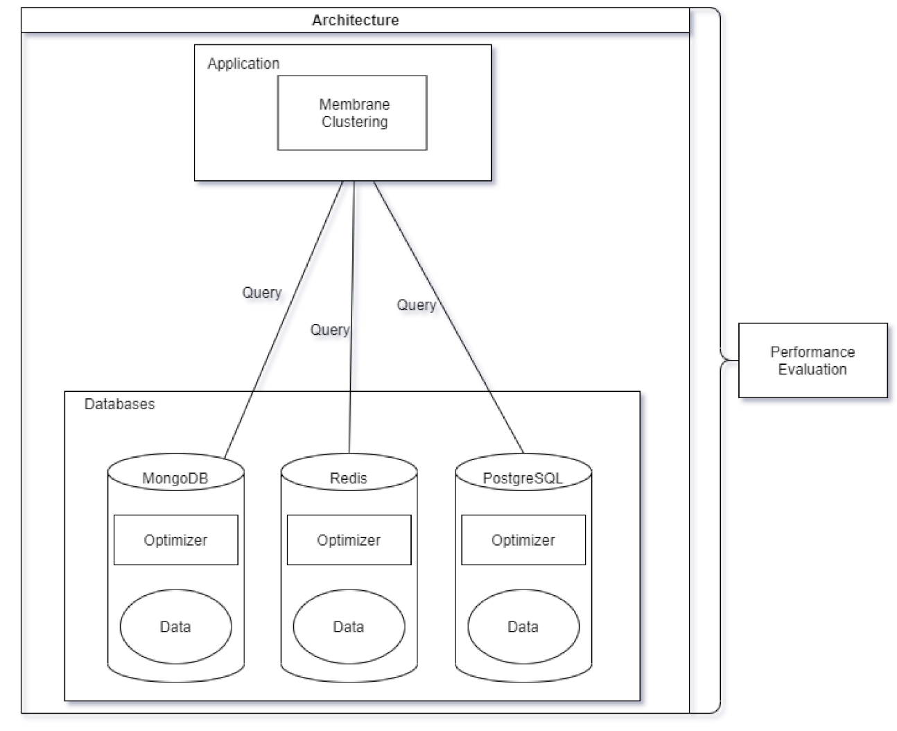
Usually, in real corporal or research environments, the data and the database management system are given, which only solves the optimization of the SQL or NoSQL queries. We suppose that this part of the system, the data, and the database manager are given, so the process must use the database manager. The performance of an application can not be lead back only to the SQL optimization, since the application can use its own methods and functions, that the SQL optimizer can not evaluate, optimize. For this reason, the performance of the applications connected to the database manager can only be measured implicitly with the called database manager as it is illustrated in Figure 1.
For this purpose, we blend the four previously described notions into a single solution, using both MongoDB and Redis. Thus, based on membrane systems with evolutionary rules, more variants (directly utilizing the two NoSQL databases) of an algorithm solving the clustering problem have been implemented and examined. The systems are compared based on experiments on the storage size required to store our data points and the running time and memory usage during the calculations. We make a suggestion about which system and how it could be utilized as a data source for membrane clustering.
The rest of this paper is arranged as follows. In Section 2.1, the previous work related to clustering algorithms is introduced, followed by Section 2.2, Section 2.3 and Section 2.4 discussing the works related to membrane systems, membrane clustering and NoSQL. Section 2.5 outlines the concerning notions in detail. Section 3.1 describes the conducted experiments, with their outcomes presented in Section 3.2. The final conclusions are gathered in Section 4.1. Lastly, in Section 4.2, possibilities are suggested for future work.
2. Materials and Methods
2.1. Clustering Algorithms
In this section, we discuss some fundamental notions and works about clustering algorithms that relate to this paper since in this paper we use a clustering algorithm. Clustering algorithms have the objective of discovering—based on a certain value, a function of goodness—groupings of a specified data set. That is, each data point in this set belongs to a group. The similarity of the members in such a cluster is maximized, while the similarity of the points in separate groups is as low as possible. There are many distinct approaches to solve the clustering problem (centroid-based, density-based, connectivity-based), each bearing its strong points. In some solutions, the number of clusters is given a priori (e.g., the well-known k-means algorithm [3]), while other variations calculate the best possible value automatically (like in the paper [4]).
Some methods result in hard clusters, where each data point is contained in exactly one group; and some in fuzzy partitions, in which case a point may belong to more clusters to a certain extent. The authors of [5] presented a survey of these. Amongst other approaches, evolutionary optimization methods have been utilized as a basis for clustering algorithms to achieve better results compared to rival solutions. Thus, numerous techniques employing simulated annealing (SA), genetic algorithm (GA), artificial bee colony (ABC), differential evolution (DE) and particle swarm optimization (PSO), or even a combination of these as their frameworks, were introduced—many of which have proven to be beneficial over other strategies.
For example, in [6], the authors proposed two new approaches using particle swarm optimization to cluster data. It finds the centroids of a specified number of clusters, then it is used with K-means clustering. The other algorithm uses particle swarm optimization to refine the clusters formed by K-means. The Artificial Bee Colony algorithm is introduced by the authors of [7], which simulates the intelligent foraging behavior of a honey bee swarm. It is used for data clustering on benchmark problems. In [8], the authors described an application of Differential Evolution to automatically cluster large unlabeled data sets. No prior knowledge is required about the data to be classified. It determines the optimal number of partitions of the data.
There are later heuristics that also can be considered: Red Fox Optimization (RFO), Polar Bear Optimization (PBO), and Chimp Optimization Algorithm (ChOA). In the method introduced in [9], the authors used a model of polar bear behaviors as a search engine for optimal solutions. The proposed simulated adaptation to harsh winter conditions is an advantage for local and global search, while the birth and death mechanism controls the population. The authors of [10] proposed a mathematical model of red fox habits, searching for food, hunting, and developing population while escaping from hunters. Their model is based on local and global optimization methods with a reproduction mechanism. In [11], a mathematical model of diverse intelligence and sexual motivation of chimps is proposed. In this regard, four types of chimps entitled attacker, barrier, chaser, and driver are employed for simulating diverse intelligence. This metaheuristic algorithm is designed to further alleviate the problems of slow convergence speed and trapping in local optima when solving high-dimensional problems. Comparing to other examined heuristics, based on [9,10,11], the results of these latest heuristics were the best in some cases while in other experiments PSO received better results, meaning PSO is still a strong heuristic.
2.2. Membrane Systems
In this section, we discuss some fundamental notions and woks about membrane systems or P systems that relate to this paper since in this paper we use a P system–based algorithm. In membrane systems, various types of membranes delimit the parts in a biological system, from the cell membrane to the skin of organisms, and virtual membranes which delimit, for instance, parts of an ecosystem. In biology and chemistry, membranes keep together certain chemicals and leave other chemicals to pass selectively. Such a system takes the form of a certain structure—a tree or an arbitrary graph, in cell-like and tissue-like membrane systems, respectively—consisting of cells as vertices, which work as parallel computing units. Each cell defines a region, containing evolution rules (delineating the calculations that may occur in the system as a sequence of transitions between its states) and a multiset of objects. A step of the computation is determined by choosing from all available rules nondeterministically, in a maximally parallel manner. When a step is applied, the system gets to a novel state or configuration; and the calculation terminates when there is no possibility for any transitions, that is, there are no rules in any of the cells that could be applied. The result of the computation may be defined by the state of a specific cell after the system halts, as they are described by the authors of [12].
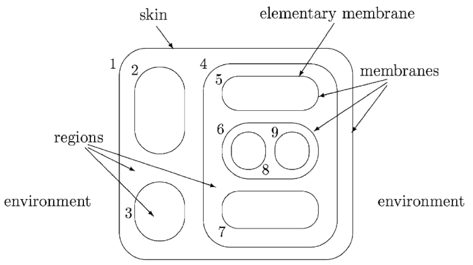
In the following, we describe the principal notions using the example of Figure 2. Membranes are arranged hierarchically in the membrane structure of a P system, embedded in a skin membrane, that separates the system from the environment. A membrane is an elementary membrane if it does not contain any membrane inside. Membranes define regions. In this example, the membranes are labeled by positive integers to make them addressable in the computations. These labels can also be used to identify the regions that the membranes delimit.
Formally P automation with membranes is a construct
where
- V is a finite alphabet of objects;
- is the output alphabet;
- is catalyst;
- is a membrane structure, containing the n membranes;
- are strings representing multisets over V associated with regions of ;
- is a finite set of evolution rules associated with region i for all i;
- is a partial order relation over
Evolution rules are pairs and can be written in the form of , where u is a string over V and where is a special symbol not in V or where is a string over .
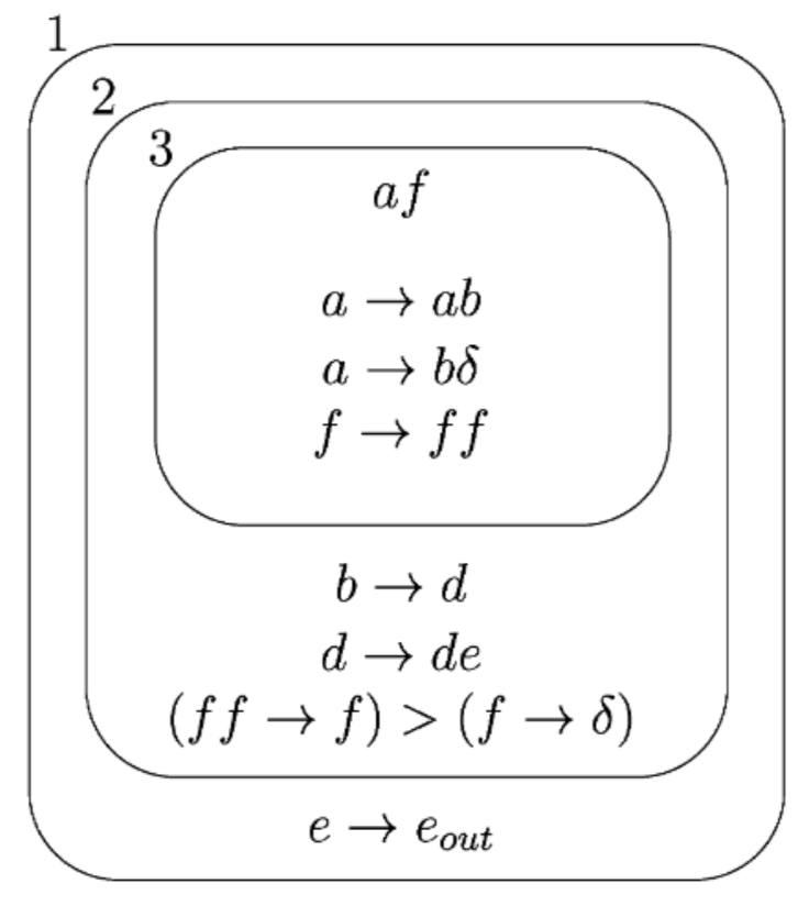
Here is a simple example initial configuration of Figure 3:
where
- , , ;
- ;
- , , ;
- , , ;
- , , ;
P systems, or membrane systems and their possibilities regarding their applications in real-life problems have been in the center of attention of many researchers over the years. They have been successfully utilized to solve numerous problems in distinct fields. Ref. [14] contains ideas on why and how purely communicating P systems can be interpreted as complex natural systems. The author gave a summary of the most relevant results concerning these P systems and provide interpretation in terms of complex systems, proposed open problems, and new directions for future research. The authors used this system in a parallel implementation for image segmenting in [15] with gradient-based edge detection in the CUDA architecture. Researchers utilized membrane system for image processing in [16]. The authors of this work presented the MAQIS membrane algorithm, where they combined membrane computing with a quantum-inspired evolutionary approach. They verified the effectiveness of their system and conducted experiments showing that it outperforms some other approaches.
In [17], the authors performed an overview of the approaches of hardware implementation in the area of P systems. They compared and evaluated quantitative and qualitative attributes of FPGA-based implementations and CUDA-enabled GPU-based simulations. The researchers used membrane computing for computational economics, where the authors of [18] designed a solution for the producer-retailer problem based on PDP systems and simulated the models in the framework by P-Lingua and MeCoSim. The authors of [19] presented the problem of spiking neural P systems having some shortcomings in numerical calculations. They combined third-generation neural network models, SNP systems with membrane computing, proposing spiking neural membrane computing models (SNMC models) to improve the implementation of SNP systems.
In [20], the authors analyzed the problems of the matrix representation of SNP systems and represented some variants of SNP systems. Based on a novel compressed representation for sparse matrices they also provided a new simulation algorithm and concluded which SNP system variant better suits their new compressed matrix representation. Boolean propositional satisfiability (SAT) problem is a widely studied NP-complete problem. In [21] the authors proposed a new algorithm for SAT problem which uses a simplification rule, the splitting rule for the traditional membrane computing algorithm of SAT problem. Based on the article, this approach can reduce time and space complexity.
P systems with antiport rules simulate register machines. In [22] the authors demonstrated three universal antiport P systems of bounded size and presented universal antiport P systems. The authors of [23] constructed simulating time Petri net to retain important characteristics of the Petri net model, that the firings of the transitions can take place in any order, and it is not needed to introduce maximal parallelism in the Petri net semantics, so they exploited the gain in computational strength obtained by the introduction of the timing feature for Petri nets.
In [24], the authors introduced the notion of a P automaton with one-way communication, a concept related both to P systems and the traditional concept of automata. They show that for any recursively enumerable language, a P automaton and a certain type of projection can be constructed such that the given language is obtained as the image of the set of accepted input multiset sequences of the P automaton. The authors of [25] proposed and preliminarily investigated the possibility of transforming a configuration of a P system into another configuration, employing a given set of rules acting both on the membranes and on the multisets of objects.
In [26], the authors constructed P colony simulating interactive processes in a reaction system, where P colonies are abstract computing devices modeling communities of very simple reactive agents living and acting in a jointly shared environment, and reaction systems were proposed as components representing basic chemical reactions that take place in a shared environment. As the last example, the authors of [27] utilized membrane computing for self-reconfigurable robots. They tested the method with computer simulations and real-world experiments too.
2.3. Membrane Clustering
In this section, we discuss some works that utilized membrane systems or P systems for clustering that relate to this paper since in this paper we use a P system–based clustering algorithm. Membrane computational models were proposed as a basis for algorithms in cluster analysis as well. Many variants of the clustering problem were solved with the help of membrane systems as frameworks, achieving highly competitive results in a lot of cases compared to their counterparts based on other approaches, in the terms of their performance and stability. The mentioned types of clustering include automatic, multi-objective, or kernel-based clustering and most proposed mechanisms use a centroid-based approach.
In [28], the authors presented a classification algorithm involving GPUs, allocating dependent objects and membranes to the same threads and thread blocks to decrease the communication between these threads and thread blocks and to allow GPUs to maintain the highest occupancy possible. In [29], the authors presented a review of 65 nature-inspired algorithms used for automatic clustering with their main components in the formulation of the metaheuristics.
In [30], the authors proposed a multiobjective clustering framework for fuzzy clustering where they designed a tissue-like membrane system. They also used artificial and real-life data for the evaluation and compared it with other techniques. To handle non-spherical cluster boundaries, the authors of [31] introduced a kernel-based membrane clustering algorithm: KMCA. It uses a tissue-like P system to determine the optimal cluster centers. The paper also includes comparisons with other algorithms. In [32], the authors introduced a clustering membrane system, named PSO-CP. It uses a cell-like P system with active membranes based on particle swarm optimization.
Most of the mentioned methods utilize nature-inspired metaheuristics—i.e., differential evolution or particle swarm optimization [33]—to describe the rules of evolution in the system that define the processes of the computation. The notion of simulated annealing has also been employed with similar intents by the authors of [34], where a partition-based clustering algorithm under the framework of membrane computing is proposed. It is based on a tissue-like P system, which is used to exploit the optimal cluster centers for a data set. The authors evaluated their approach on artificial and real-life data sets and compared it with approaches based on k-means. In the end, after surveying the related works about membrane clustering, we decided to base our algorithm on the solution presented in [35], which is going to be described in more detail.
2.4. NoSQL
In the following section, we explore some of the works that investigated NoSQL, MongoDB, and Redis too. As the authors of [36] describe Redis, Redis is a data structure server with an in-memory data set for speed. It is not a simple key-value store, it implements data structures allowing keys to containing for example binary-safe strings, hashes, sets, and sorted sets, or lists. Based on [37] the developers of MongoDB aimed to create a database that worked with documents, usually with JSON in this case, and that was fast, scalable, and easy to use.
The authors of [38] used a combination of NoSQL databases applied to information management systems to replace traditional databases like Oracle, comparing the traditional database system with the combination of MongoDB and Redis and presented the performance comparison of these two schemas. In [39], the authors compared different NoSQL databases and evaluated their performance according to the typical usage for storing and retrieving data. They tested 10 NoSQL databases using a mix of operations with Yahoo! Cloud Serving Benchmark to understand how performance is affected by each database type and their internal mechanisms and to understand the capability of the examined databases for handling different requests. Based on their work, MongoDB, Redis, Scalaris, Tarantool, and OrientDb are optimized for read operations among the 10 databases evaluated, which is important for our work, since we are going to inspect the databases while handling read requests for clustering.
The authors of [40] proposed a comparative classification model that relates requirements to techniques and algorithms employed in NoSQL databases. Their NoSQL Toolbox allows deriving a simple decision tree to help filter potential system candidates based on central application requirements. In [41] authors compared MongoDB, Cassandra, Redis and Neo4j. They found that write and delete operations are fast for MongoDB, Redis, and Cassandra, while the read operation is comparatively slow in Cassandra. They also discussed how these databases work in a distributed environment.
According to [42] NoSQL databases can be divided into four categories: key-value store, document store, column family, and graph database. Based on [43], graph databases should not be evaluated according to the scenarios used in the analysis of the other types of NoSQL databases, because the usage of links between records requires a different approach. We decided to use MongoDB and Redis, considering this and the evaluations above.
Besides the works discussed above, there are already many comparisons available about the performance of the NoSQL databases. In this paper, we are interested in the utilization of NoSQL databases for P system-based clustering and how these databases perform when using them under P system-based clustering. So we conducted experiments where we inspect this algorithm while using the NoSQL databases as data sources. This issue had not been discussed in the related works.
2.5. The Used Algorithm
In this section, we describe the implemented algorithm used in this paper, which is based on the foundation introduced in [35]. Its goal is to attain a solution to a clustering problem, detailed in the following. Given a data set , composed of n data points. These points are laid out in a d-dimensional Euclidean space, i.e., for each point in X, . The number of the required clusters, K, is known a priori. However, no prior information is available with respect to the likeness of the points in X.
The objective is to find a grouping for the data points, such that all points belong to one of K distinct groups. The similarity of the data points inside a group, and the dissimilarity of the points between different groups, are maximized. The resemblance amongst the points is defined by a certain similarity measure: a clustering validity index. The algorithm in the mentioned paper [35] describes a tissue-like membrane system model with evolutionary and communicational rules as its basis to acquire a solution to the previously defined clustering problem.
Definition 1.
A tissue-like membrane system or tissue P system of degree is a construct
where
- O is a finite, non-empty alphabet of objects;
- μ describes the (graph) structure, containing the p nested cells;
- is a finite multiset of objects over O, contained by cell i of μ in the initial state of the calculation;
- is a finite set of evolutionary rules contained by cell i of μ;
- is finite set of communicational rules between the cells of μ; and finally
- specifies the cell accommodating the output of the computation (if , the region outside the outer cell contains the output).
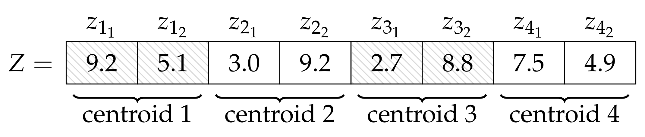
The succession of steps, as changes in the state of the system, form the computation itself. In these steps, the applicable rules are selected and then applied in every cell in a maximally parallel manner. The objects in each cell are evolved according to their own evolution rules and—through the help of communication rules—the achieved results of the other cells. Local best objects in each cell and the global best object over all of the cells are updated, stored, and utilized during the steps. The centroids of the K clusters are denoted by the objects contained in each cell. An object is a vector containing the K potential cluster centroids. These are d-dimensional points in a Euclidean space, thus . An example of Z can be seen in Figure 4. In the initial state of our algorithm, every single centroid contained in the objects of each cell is equal to a randomly chosen data point from the data set X.
The main component of the system is the evolutionary rules. They define the alterations that take place during the steps of the algorithm. In [35], the mechanisms introduced in the PSO method [33] provide the foundation of these rules that move the cluster centroids. For each object i contained in cell j (denoted by ), the following changes are applied during the computation:
The values above are input parameters of the method; while are random real numbers from the range of 0 to 1. In the implementation these are generated by the random python module. The value of w is calculated as follows:
where and are input parameters, the latter indicating the number of steps taken by the system. The value t corresponds to the number of steps taken at the given moment.
Lastly, in Equation (1), the object denotes the best position of the object found thus far, stands for the local best object in cell i, and is a randomly selected object (from the set of obtained—through the communicational rules—best objects of all other cells in the system), called the external best object. The aforementioned three objects and the global best object are calculated (and compared) based on a specific measure of quality—the clustering validity index. The FCM (Fuzzy C-Means) measure is employed in our case, since it produces generally good outcomes, while it can be efficiently calculated. indicates this value for K clusters, defined below.
In the preceding equation, stands for the Euclidean norm and the values of the fuzzy partition matrix u are the following:
Last, but not least, the computation defined so far terminates, when the amount of steps taken reaches the value specified in . At this point, the desired cluster centroids are contained in the global best object, with which the data points can be classified into the appropriate groups. The following algorithm, that was used for the experiments, first initializes the cells and the best position values for each object. After that, the objects of the cells are evolved and the best positions are updated. Lastly, the global best position is updated. This is repeated until reaching steps. The global best positions are found as the optimal cluster centers.
Pseudo code:
BEGIN
Initialize cells and best positions
WHILE step < tmax DO
FOR each cell DO
FOR each object DO
CALL update_best_position()
END
END
FOR each cell DO
IF best in cell < global best THEN
Update global best
END
END
Increase step
END
RETURN global best positions
END
FUNCTION update_best_position() BEGIN
Calculate w using Equation~(2)
Evolve object using Equation~(1)
Calculate partition matrix using Equation~(4)
Calculate FCM using Equation~(3)
IF FCM for given object < best so far THEN
Update best position for object
END
END
The maximal clustering performance was analyzed over different configurations of the system with Davies–Bouldin, Calinski–Harabasz and Silhouette indexes. We also experienced with the parameters of the algorithm used in this paper and measured with the Calinski–Harabasz index how these should be set in our previous paper [44]. We reached good average clustering validity scores with the combination of , , , , , . In the experiments we used these parameters.
Using a simple example object: , denoted by and the suggested input parameters, we present the first step of the evolution of the object.
First, we calculate w using Equation (2):
Since the steps are indexed from zero and we are in the first, here .
Here we suppose that we found as the best position of the object, as a local best object in the cell and is a randomly selected object.
Now adding the components, we get the velocity:
Lastly, we get the evolved object by adding the velocity:
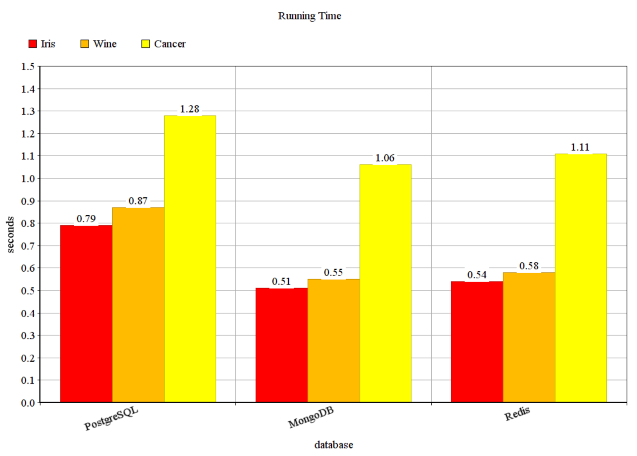
In our previous paper [44], we made some experiments using the PostgreSQL database management system on three different datasets (Iris, Wine Recognition, and Breast Cancer Wisconsin (Diagnostic) datasets) from the well-known UCI Machine Learning Repository [45]. However, in big data applications, usually, NoSQL systems are utilized, since some of the frequent operations may be faster in such systems, as it is already mentioned earlier and as it is discussed in [2]. In Figure 5, some preliminary measurements can be seen, comparing the running times measured in the previous paper using PostgreSQL with the measurements made for this paper using the MongoDB and Redis database management systems. Since the NoSQL database management systems perform much better, the results of this experiment also prove the need for the change of the database management system supporting the clustering. The Iris dataset contains 150 points in 4 dimensions, the Wine dataset 178 points in 13 dimensions, and the cancer dataset 569 points in 30 dimensions. To compare the NoSQL database management systems, later we generated larger datasets.
3. Results
3.1. Experiments
The algorithm used in this paper was implemented in Python 3, with the help of the pymongo and the redis packages for directly accessing the MongoDB and Redis databases. The data points used by the P system in the experiments are structured in the following way. In MongoDB, a collection, which is a JSON document, corresponds to a collection of points. In this document, each line corresponds to a point, where the dimensions of the point are listed with their values.
Example data points in MongoDB:
{“d1”: 5.68, “d2”: 0.35, “d3”: 3.12, …}
{“d1”: −0.83, “d2”: 3.67, “d3”: 1.12, …}
{“d1”: −6.48, “d2”: −7.1, “d3”: 4.89, …}
…
In Redis, each point corresponds to a list, where the elements of the list correspond to the positions of the point in the different dimensions. The key of each list is built up by the name of the point collection and the point identifier delimited by: symbol.
Example data points in Redis:
collection1:point1 5.68 0.35 3.12 …
collection1:point2 −0.83 3.67 1.12 …
collection1:point3 −6.48 −7.1 4.89 …
…
To test our solutions with larger data sets, we generated data sets of 10,000, 20,000 data points in 100–500 dimensions for the memory usage experiments and 100,000, 200,000, 300,000 data points in 10, 20, 30 dimensions for the running time experiments using the make_blobs function of the sklearn [46] python module. We loaded the data by generating JSON files, then importing them into MongoDB. In the case of Redis, we connected to the database through python and loaded the data by calling the lpush Redis operation. To query the databases we used the find MongoDB operation and the lrange Redis operation. During the calculation, each point was stored in numpy arrays.
Memory usage during the calculation was measured by the RSS of the memory_info function of the Process in the psutil python module. RSS is the “Resident Set Size”, the non-swapped physical memory a process has used. The measurements were made on Intel(R) Core(TM) i5-1035G1 CPU with 8 GB RAM.
3.2. Evaluation
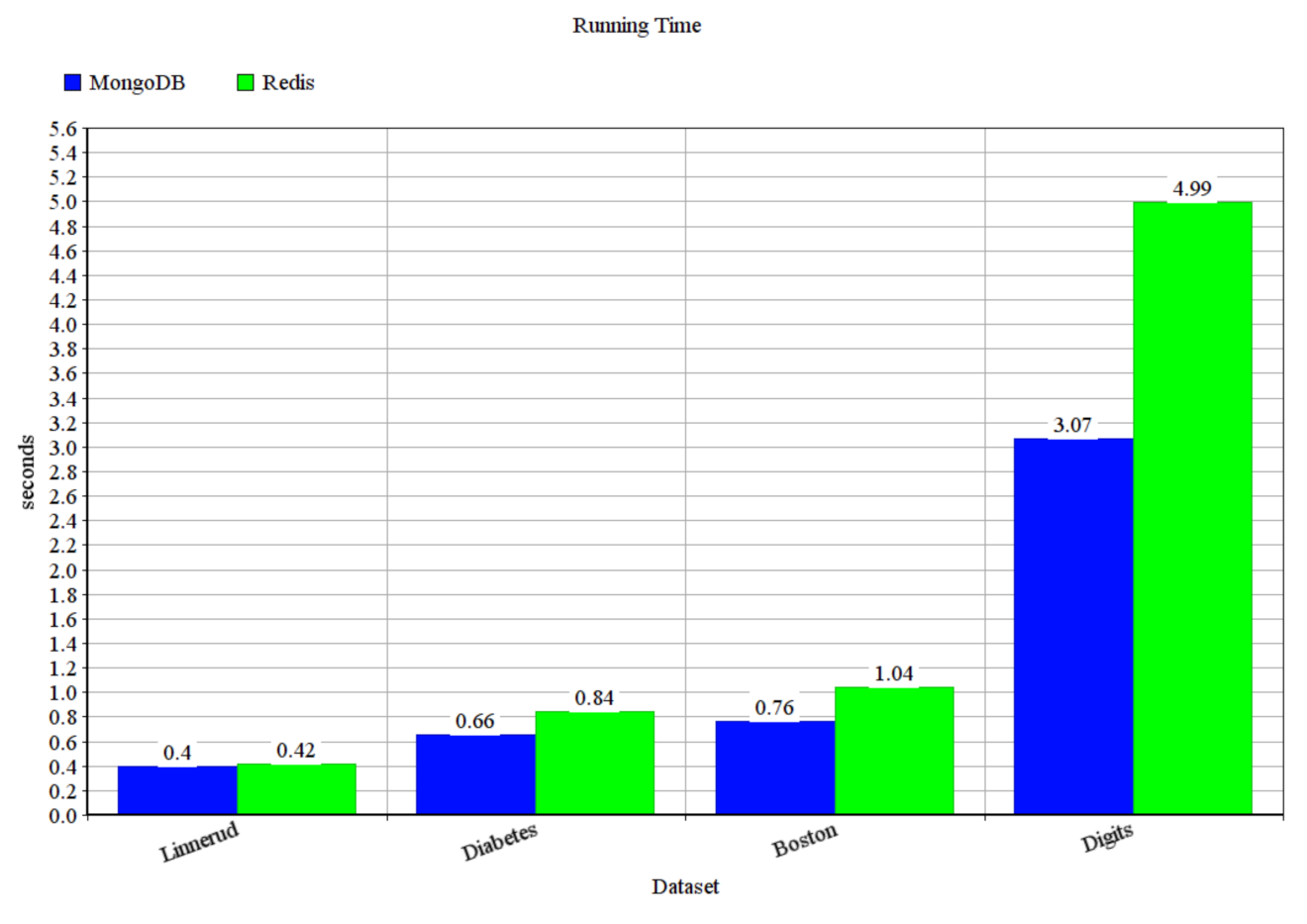
To compare the performance of MongoDB and Redis NoSQL database management systems serving as data sources for our membrane clustering solution, we measured the size required to store the data points, the running time, and the memory consumption of the systems. First, we made some experiments with more well-known datasets: Linnerud containing 20 points in 3 dimensions, Diabetes containing 442 points in 10 dimensions, Boston containing 506 points in 13 dimensions, and Digits containing 1797 points in 64 dimensions from the UCI Machine Learning Repository [45]. The results are presented in Figure 6, where it can be seen that MongoDB performs better than Redis. However, since we use NoSQL database management systems, we are more interested in using them on larger datasets. In the following experiments, we used our generated datasets for this purpose.
In Figure 7, we can inspect the storage size in MongoDB and Redis after loading our data points in kilobytes for the different combinations of the number of data points and point dimensions. It can be seen, that MongoDB could store the data in a much smaller size, moreover, it scales much better than Redis, in this aspect. When storing 100,000 data points in 10 dimensions, the difference is small, but in MongoDB, the storage size is already smaller. When storing 300,000 data points in 30 dimensions, the difference grew much larger, favoring MongoDB.
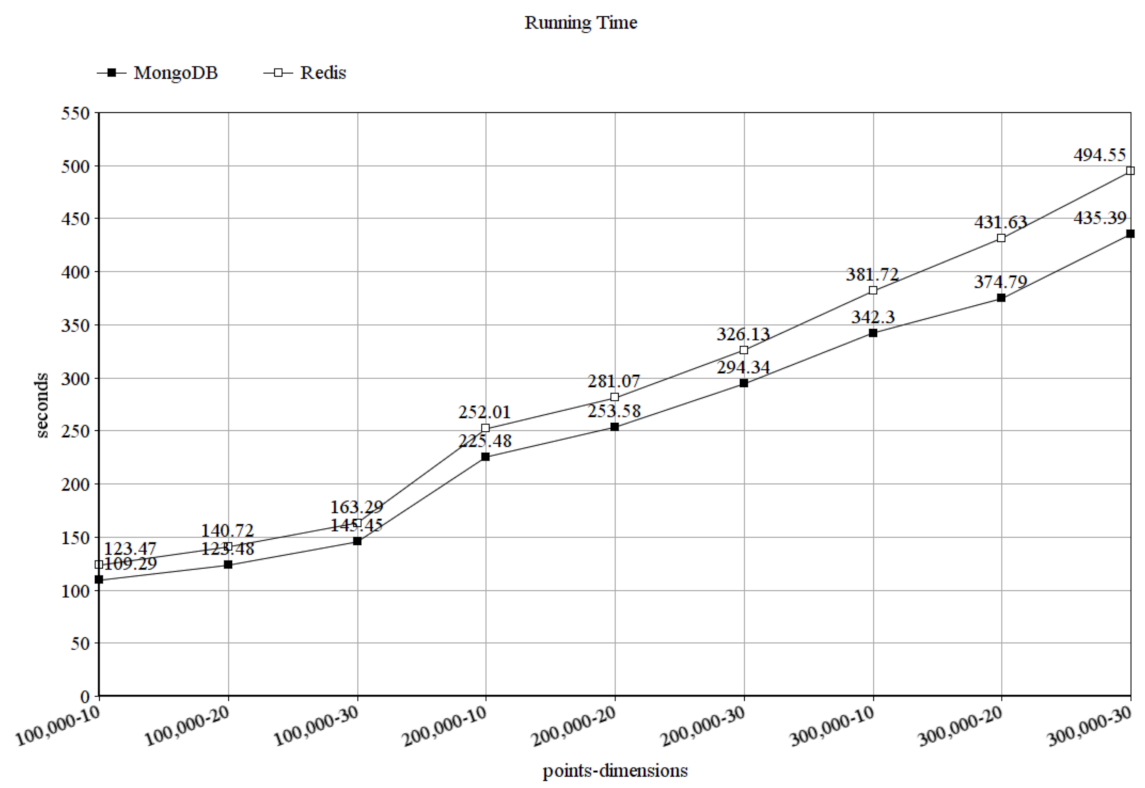
Based on our experiments, in Figure 8 we can see that MongoDB was also faster than Redis while solving the membrane clustering task and it scaled better than Redis. Since the running time is measured while running the same algorithm with different databases, this means that MongoDB loads the data faster than Redis. The figure shows how much time it took to solve the clustering problem in seconds, again with the different combinations of the number of data points and point dimensions. Here, the difference is not that great, compared to the measurements in storage size, but it can be seen, that again, when using 100,000 data points in 10 dimensions, MongoDB was slightly faster than Redis; however, when using 300,000 data points in 30 dimensions, the difference slightly grew and it would grow further in case of more points and dimensions.
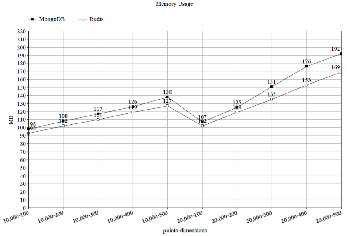
To measure the memory usage, we increased the number of dimensions to 100–500, because the difference in the memory usage stayed similar when we just increased the number of data points. In Figure 9, showing the memory usage in bytes, it can be seen that MongoDB used more memory than Redis and also Redis scaled better in this aspect. While Redis is an in-memory database, meaning it loads all data that it wants to work with into the memory, the memory usage of MongoDB could be decreased by loading smaller data chunks into the memory and write intermediate states of the membranes to disk. However, of course, it would increase the running time, since disk operations are usually very expensive.
4. Discussion and Conclusions
4.1. Conclusions
In this paper, we were experimenting with how to use a membrane clustering algorithm over NoSQL database management systems and which of these systems should be used for such purposes. Since the methods and functions of an application can not be evaluated and optimized by the SQL optimizer, we conducted some experiments using MongoDB and Redis, connected to our membrane clustering algorithm, with generated data sets and evaluated them, based on the storage size of the stored data points in these systems, the running time, and memory usage while solving the membrane clustering task. In conclusion, based on the results of our experimental comparison, both MongoDB and Redis have their advantages and disadvantages. Overall, considering the disadvantage of MongoDB can be decreased in the cost of the running time, we would recommend using MongoDB as a data source for membrane clustering data points.
4.2. Future Work
Considering that membrane systems are parallel computing models, the algorithm should also be tested with parallel implementation. To do this, python gives some possibilities for parallel computing, but big data platforms like Spark could also be used to distribute the computing to computational nodes. Considering the data source, as we mentioned MongoDB working with smaller data chunks, other database management systems or data models should be evaluated or, if we do not already have all data to cluster, membrane clustering with data flows could also be investigated. Furthermore, the integration of other evolutionary optimization techniques into our current solution should be tested.
Author Contributions
Conceptualization, P.L.-K., T.T. and A.K.; methodology, P.L.-K., T.T. and A.K.; software, P.L.-K., T.T.; validation, P.L.-K., T.T. and A.K.; investigation, P.L.-K., T.T. and A.K.; writing—original draft preparation, P.L.-K., T.T. and A.K.; writing—review and editing, P.L.-K., T.T. and A.K.; supervision, A.K.; project administration, A.K. All authors have read and agreed to the published version of the manuscript.
Funding
The project has been supported by the European Union, co-financed by the European Social Fund (EFOP-3.6.3-VEKOP-16-2017-00002). This research was also supported by grants of “Application Domain Specific Highly Reliable IT Solutions” project that has been implemented with the support provided from the National Research, Development and Innovation Fund of Hungary, financed under the Thematic Excellence Programme TKP2020-NKA-06 (National Challenges Subprogramme) funding scheme.
Institutional Review Board Statement
Not applicable.
Informed Consent Statement
Not applicable.
Data Availability Statement
Conflicts of Interest
The authors declare no conflict of interest.
Abbreviations
The following abbreviations are used in this manuscript:
| SA | Simulated Annealing |
| GA | Genetic Algorithm |
| ABC | Artificial Bee Colony |
| DE | Differential Evolution |
| PSO | Particle Swarm Optimization |
| RFO | Red Fox Optimization |
| PBO | Polar Bear Optimization |
| ChOA | Chimp Optimization Algorithm |
| CUDA | Compute Unified Device Architecture |
| MAQIS | Membrane Algorithm with Quantum-Inspired Subalgorithms |
| FPGA | Field Programmable Gate Arrays |
| PDP | Programmed Data Processor |
| MeCoSim | Membrane Computing Simulator |
| SNP | Spiking Neural P Systems |
| SNMC | Spiking Neural Membrane Computing |
| SAT problem | Boolean Satisfiability Problem |
| KMCA | Kernel-based Membrane Clustering Algorithm |
| PSO-CP | Particle Swarm Optimization Cell-like P system |
| FCM | Fuzzy C-Means |
| RSS | Resident Set Size |
| UCI | University of California, Irvine |
References
- Păun, G. Computing with Membranes. J. Comput. Syst. Sci. 2000, 61, 108–143. [Google Scholar] [CrossRef] [Green Version]
- Li, Y.; Manoharan, S. A performance comparison of SQL and NoSQL databases. In Proceedings of the 2013 IEEE Pacific Rim Conference on Communications, Computers and Signal Processing (PACRIM), Vancouver, BC, Canada, 27–29 August 2013; pp. 15–19. [Google Scholar]
- MacQueen, J. Some methods for classification and analysis of multivariate observations. In Proceedings of the 5th Berkeley Symposium on Mathematical Statistics and Probability, Oakland, CA, USA, 1 January 1967; Volume 1, pp. 281–297. [Google Scholar]
- Hamerly, G.; Elkan, C. Learning the k in k-means. In Advances in Neural Information Processing Systems; MIT Press: Cambridge, MA, USA; London, UK, 2004; pp. 281–288. [Google Scholar]
- Xu, R.; Wunsch, D. Survey of clustering algorithms. IEEE Trans. Neural Netw. 2005, 16, 645–678. [Google Scholar] [CrossRef] [PubMed] [Green Version]
- van der Merwe, D.W.; Engelbrecht, A.P. Data clustering using particle swarm optimization. In Proceedings of the 2003 Congress on Evolutionary Computation (CEC ’03), Canberra, ACT, Australia, 8–12 December 2003; Volume 1, pp. 215–220. [Google Scholar] [CrossRef]
- Karaboga, D.; Ozturk, C. A novel clustering approach: Artificial bee colony (ABC) algorithm. Appl. Soft Comput. 2010, 11, 652–657. [Google Scholar] [CrossRef]
- Das, S.; Abraham, A.; Konar, A. Automatic clustering using an improved differential evolution algorithm. IEEE Trans. Syst. Man Cybern. Part A Syst. Hum. 2007, 38, 218–237. [Google Scholar] [CrossRef]
- Połap, D. Polar bear optimization algorithm: Meta-heuristic with fast population movement and dynamic birth and death mechanism. Symmetry 2017, 9, 203. [Google Scholar] [CrossRef] [Green Version]
- Połap, D.; Woźniak, M. Red fox optimization algorithm. Expert Syst. Appl. 2021, 166, 114107. [Google Scholar] [CrossRef]
- Khishe, M.; Mosavi, M.R. Chimp optimization algorithm. Expert Syst. Appl. 2020, 149, 113338. [Google Scholar] [CrossRef]
- Păun, G. Membrane Computing—An Introduction; Springer: Berlin/Heidelberg, Germany, 2002. [Google Scholar]
- Păun, G.; Rozenberg, G. A guide to membrane computing. Theor. Comput. Sci. 2002, 287, 73–100. [Google Scholar] [CrossRef] [Green Version]
- Csuhaj-Varjú, E. Communicating P Systems: Bio-inspired Computational Models for Complex Systems. In Proceedings of the CEUR Workshop Proceedings, Oravská Lesná, Slovakia, 18–22 September 2020; pp. 3–8. [Google Scholar]
- Díaz-Pernil, D.; Berciano, A.; PeñA-Cantillana, F.; GutiéRrez-Naranjo, M.A. Segmenting images with gradient-based edge detection using membrane computing. Pattern Recognit. Lett. 2013, 34, 846–855. [Google Scholar] [CrossRef]
- Zhang, G.; Gheorghe, M.; Li, Y. A membrane algorithm with quantum-inspired subalgorithms and its application to image processing. Nat. Comput. 2012, 11, 701–717. [Google Scholar] [CrossRef]
- Zhang, G.; Shang, Z.; Verlan, S.; Martínez-del Amor, M.Á.; Yuan, C.; Valencia-Cabrera, L.; Pérez-Jiménez, M.J. An overview of hardware implementation of membrane computing models. ACM Comput. Surv. (CSUR) 2020, 53, 1–38. [Google Scholar] [CrossRef]
- Sánchez Karhunen, E.; Valencia Cabrera, L. Membrane Computing Applications in Computational Economics. In Proceedings of the BWMC 2017: 15th Brainstorming Week on Membrane Computing, Andalusia, Spain, 31 January–3 February 2017; pp. 189–214. [Google Scholar]
- Liu, X.; Ren, Q. Spiking Neural Membrane Computing Models. Processes 2021, 9, 733. [Google Scholar] [CrossRef]
- Martínez-del Amor, M.Á.; Orellana-Martín, D.; Pérez-Hurtado, I.; Cabarle, F.G.C.; Adorna, H.N. Simulation of Spiking Neural P Systems with Sparse Matrix-Vector Operations. Processes 2021, 9, 690. [Google Scholar] [CrossRef]
- Hao, L.; Liu, J. Enhanced Membrane Computing Algorithm for SAT Problems Based on the Splitting Rule. Symmetry 2019, 11, 1412. [Google Scholar] [CrossRef] [Green Version]
- Csuhaj-Varjú, E.; Margenstern, M.; Vaszil, G.; Verlan, S. On small universal antiport P systems. Theor. Comput. Sci. 2007, 372, 152–164. [Google Scholar] [CrossRef] [Green Version]
- Battyányi, P.; Vaszil, G. Description of membrane systems with time Petri nets: Promoters/inhibitors, membrane dissolution, and priorities. J. Membr. Comput. 2020, 2, 341–354. [Google Scholar] [CrossRef]
- Csuhaj-Varjú, E.; Vaszil, G. P automata or purely communicating accepting P systems. In Workshop on Membrane Computing; Springer: Berlin/Heidelberg, Germany, 2002; pp. 219–233. [Google Scholar]
- Csuhaj-Varjú, E.; Nola, A.D.; Păun, G.; Pérez-Jiménez, M.J.; Vaszil, G. Editing configurations of P systems. Fundam. Inform. 2008, 82, 29–46. [Google Scholar]
- Ciencialová, L.; Cienciala, L.; Csuhaj-Varjú, E. P colonies and reaction systems. J. Membr. Comput. 2020, 2, 269–280. [Google Scholar] [CrossRef]
- Bie, D.; Gutiérrez-Naranjo, M.A.; Zhao, J.; Zhu, Y. A membrane computing framework for self-reconfigurable robots. Nat. Comput. 2019, 18, 635–646. [Google Scholar] [CrossRef]
- Muniyandi, R.C.; Maroosi, A. A Representation of Membrane Computing with a Clustering Algorithm on the Graphical Processing Unit. Processes 2020, 8, 1199. [Google Scholar] [CrossRef]
- José-García, A.; Gómez-Flores, W. Automatic clustering using nature-inspired metaheuristics: A survey. Appl. Soft Comput. 2016, 41, 192–213. [Google Scholar] [CrossRef]
- Peng, H.; Shi, P.; Wang, J.; Riscos-Núñez, A.; Pérez-Jiménez, M. Multiobjective fuzzy clustering approach based on tissue-like membrane systems. Knowl.-Based Syst. 2017, 125. [Google Scholar] [CrossRef]
- Yang, J.; Chen, R.; Zhang, G.; Peng, H.; Wang, J.; Riscos-Núñez, A. A. A kernel-based membrane clustering algorithm. In Enjoying Natural Computing; Springer: Berlin/Heidelberg, Germany, 2018; pp. 318–329. [Google Scholar]
- Wang, L.; Liu, X.; Sun, M.; Qu, J. An Extended clustering membrane system based on particle swarm optimization and cell-like P system with active membranes. Math. Probl. Eng. 2020, 2020, 5097589. [Google Scholar] [CrossRef] [Green Version]
- Kennedy, J. Particle Swarm Optimization. In Encyclopedia of Machine Learning; Sammut, C., Webb, G.I., Eds.; Springer: Boston, MA, USA, 2010. [Google Scholar] [CrossRef]
- Jiang, Y.; Peng, H.; Huang, X.; Zhang, J.; Shi, P. A novel clustering algorithm based on P systems. Int. J. Innov. Comput. Inf. Control. IJICIC 2014, 10, 753–765. [Google Scholar]
- Peng, H.; Wang, J.; Shi, P.; Riscos-Núñez, A.; Pérez-Jiménez, M.J. An automatic clustering algorithm inspired by membrane computing. Pattern Recognit. Lett. 2015, 68, 34–40. [Google Scholar] [CrossRef]
- Macedo, T.; Oliveira, F. Redis Cookbook: Practical Techniques for Fast Data Manipulation; O’Reilly Media, Inc.: Sebastopol, CA, USA, 2011. [Google Scholar]
- Plugge, E.; Hows, D.; Membrey, P.; Hawkins, T. The Definitive Guide to MongoDB: A Complete Guide to Dealing with Big Data Using MongoDB; Apress: New York, NY, USA, 2015. [Google Scholar]
- Punia, Y.; Aggarwal, R. Implementing Information System Using MongoDB and Redis. Int. J. Adv. Trends Comput. Sci. Eng. 2014, 3, 16–20. [Google Scholar]
- Abramova, V.; Bernardino, J.; Furtado, P. Experimental evaluation of NoSQL databases. Int. J. Database Manag. Syst. 2014, 6, 1. [Google Scholar] [CrossRef]
- Gessert, F.; Wingerath, W.; Friedrich, S.; Ritter, N. NoSQL database systems: A survey and decision guidance. Comput. Sci.-Res. Dev. 2017, 32, 353–365. [Google Scholar] [CrossRef]
- Gupta, A.; Tyagi, S.; Panwar, N.; Sachdeva, S.; Saxena, U. NoSQL databases: Critical analysis and comparison. In Proceedings of the IEEE 2017 International Conference on Computing and Communication Technologies for Smart Nation (IC3TSN), Gurgaon, India, 12–14 October 2017; pp. 293–299. [Google Scholar]
- Indrawan-Santiago, M. Database research: Are we at a crossroad? Reflection on NoSQL. In Proceedings of the IEEE 2012 15th International Conference on Network-Based Information Systems, Melbourne, VIC, Australia, 26–28 September 2012; pp. 45–51. [Google Scholar]
- Armstrong, T.G.; Ponnekanti, V.; Borthakur, D.; Callaghan, M. LinkBench: A database benchmark based on the Facebook social graph. In Proceedings of the 2013 ACM SIGMOD International Conference on Management of Data, New York, NY, USA, 22–27 June 2013; pp. 1185–1196. [Google Scholar]
- Tarczali, T.; Lehotay-Kéry, P.; Kiss, A. Membrane Clustering Using the PostgreSQL Database Management System. In Proceedings of the SAI Intelligent Systems Conference; Springer: Berlin/Heidelberg, Germany, 2020; pp. 377–388. [Google Scholar]
- Dua, D.; Graff, C. UCI Machine Learning Repository. Available online: http://archive.ics.uci.edu/ml (accessed on 27 July 2021).
- Pedregosa, F.; Varoquaux, G.; Gramfort, A.; Michel, V.; Thirion, B.; Grisel, O.; Blondel, M.; Prettenhofer, P.; Weiss, R.; Dubourg, V.; et al. Scikit-learn: Machine Learning in Python. J. Mach. Learn. Res. 2011, 12, 2825–2830. [Google Scholar]
Figure 1.
System architecture.

Figure 2.
Example membrane structure [13].
Figure 2.
Example membrane structure [13].

Figure 3.
Example initial configuration [13].
Figure 3.
Example initial configuration [13].

Figure 4.
An example of an object in the system, with values and .

Figure 5.
Running time in seconds.

Figure 6.
Running time in seconds.

Figure 7.
Storage size in megabytes.

Figure 8.
Running time in seconds.

Figure 9.
Memory usage in megabytes.

Publisher’s Note: MDPI stays neutral with regard to jurisdictional claims in published maps and institutional affiliations. |
© 2021 by the authors. Licensee MDPI, Basel, Switzerland. This article is an open access article distributed under the terms and conditions of the Creative Commons Attribution (CC BY) license (https://creativecommons.org/licenses/by/4.0/).
Share and Cite
MDPI and ACS Style
Lehotay-Kéry, P.; Tarczali, T.; Kiss, A. P System–Based Clustering Methods Using NoSQL Databases. Computation 2021, 9, 102. https://0-doi-org.brum.beds.ac.uk/10.3390/computation9100102
AMA Style
Lehotay-Kéry P, Tarczali T, Kiss A. P System–Based Clustering Methods Using NoSQL Databases. Computation. 2021; 9(10):102. https://0-doi-org.brum.beds.ac.uk/10.3390/computation9100102
Chicago/Turabian StyleLehotay-Kéry, Péter, Tamás Tarczali, and Attila Kiss. 2021. "P System–Based Clustering Methods Using NoSQL Databases" Computation 9, no. 10: 102. https://0-doi-org.brum.beds.ac.uk/10.3390/computation9100102
Note that from the first issue of 2016, this journal uses article numbers instead of page numbers. See further details here.