
Assessment of SQL and NoSQL Systems to Store and Mine COVID-19 Data


1
Polytechnic of Coimbra, Coimbra Institute of Engineering (ISEC), 3030-199 Coimbra, Portugal
2
Centre of Informatics and Systems of University of Coimbra (CISUC), 3030-290 Coimbra, Portugal
3
FATEC Mogi das Cruzes, São Paulo Technological College, Mogi das Cruzes 08773-600, Brazil
*
Author to whom correspondence should be addressed.
Computers 2022, 11(2), 29; https://0-doi-org.brum.beds.ac.uk/10.3390/computers11020029
Submission received: 15 December 2021
/
Revised: 11 February 2022
/
Accepted: 15 February 2022
/
Published: 21 February 2022
Abstract
:COVID-19 has provoked enormous negative impacts on human lives and the world economy. In order to help in the fight against this pandemic, this study evaluates different databases’ systems and selects the most suitable for storing, handling, and mining COVID-19 data. We evaluate different SQL and NoSQL database systems using the following metrics: query runtime, memory used, CPU used, and storage size. The databases systems assessed were Microsoft SQL Server, MongoDB, and Cassandra. We also evaluate Data Mining algorithms, including Decision Trees, Random Forest, Naive Bayes, and Logistic Regression using Orange Data Mining software data classification tests. Classification tests were performed using cross-validation in a table with about 3 M records, including COVID-19 exams with patients’ symptoms. The Random Forest algorithm has obtained the best average accuracy, recall, precision, and F1 Score in the COVID-19 predictive model performed in the mining stage. In performance evaluation, MongoDB has presented the best results for almost all tests with a large data volume.
1. Introduction
The human species has already witnessed several pandemics during its existence. A pandemic is an epidemic occurring on a scale that crosses international boundaries, usually affecting many people [1]. In December 2019, the first case of COVID-19, the most recent pandemic, appeared in China. The clinical features of the first patients to be infected with COVID-19 included lower respiratory tract illness with fever, dry cough, and dyspnea. COVID-19 was declared a pandemic in March 2020 and quickly became a worldwide public health and social security hazard [2]. Today, the virus is still responsible for severe impacts, with a continuous increase in the confirmed number of cases and deaths. According to the World Health Organization (WHO), about 250 million people were infected, including more than 5 million deaths [3].
The advent of COVID-19 vaccine has significantly reduced confirmed cases, hospitalizations, and deaths. In Israel, vaccine effectiveness against symptomatic SARS-CoV-2 infection, hospitalizations, and deaths exceeded 96% across all age groups, including older ages (75 plus years old) [4]. Despite the improvements, we are still far from being safe from this pandemic, so we must continue to make efforts and work together on the way out. Moreover, while the world is still reeling from the COVID-19 pandemic, public health organizations are already promoting in-depth studies that scrutinize the characteristics of the current health crisis to prevent another one in the future.
Artificial Intelligence (AI) methods have been successfully used to solve many problems in healthcare. Healthcare organizations are currently capable of collecting a large amount of data that can be used to generate helpful insights once mined. Data Mining is an advanced artificial intelligence technique used for discovering novel, useful, and valid hidden patterns or knowledge from datasets [5,6]. The acquired knowledge through this process has been improving work efficiency and strengthening decision-making. Data Mining is gaining popularity in distinct research fields due to its boundless applications and approaches [7].
In this work, Data Mining algorithms were used in classification problems to extract insights from the collected data and develop a COVID-19 predictive model with suitable accuracy. In the experiments, we apply Decision Tree, Naive Bayes, Neural Network, and Logistic Regression algorithms using Orange Data Mining [8] to mine the data.
Over the years, the evolution of organizations has led to the need to respond quickly to new environmental and market challenges. In addition, the massive volume of stored data requires databases adapted to corporate needs that efficiently process the entire datasets.
Non-relational databases, known as NoSQL databases, have emerged to fill this gap [9]. NoSQL technology helps programmers and IT professionals manage the new challenges of the models and the diversity of data types. Unpredictable data are processed extremely effectively, achieving a very fast query runtime. In addition, NoSQL databases bring additional features that distinguish them from relational databases, known as SQL databases. Namely, they do not require rigid database schema to be defined and retain easy horizontal scalability [10].
In this paper, we evaluate one SQL database, Microsoft SQL Server [11], and two of the most popular NoSQL databases, MongoDB [12] and Cassandra [13]. This evaluation was performed using real COVID-19 datasets by comparing the different databases in terms of query runtime, RAM consumed, CPU percentage used, and data storage size.
COVID-19 took everyone by surprise and has posed tremendous challenges to many aspects of human lives and activities, causing damage worldwide. Therefore, the human population must be prepared for the eventuality of the next pandemic. The motivation of this work is to present the best data technology to store, handle, and mine COVID-19 data, create a COVID-19 predictive model, and select the best algorithm. Therefore, the first goal of this work is to create a COVID-19 database and mine it to extract insights from the data. The second goal is evaluating which of the different used databases is the best for storing and mining COVID-19 data.
The remaining sections are organized as follows. Section 2 reviews related work on SQL versus NoSQL databases and Data Mining on COVID-19 data. Section 3 describes Data Mining and the algorithms used in the experiments. Section 4 describes creating the database and inserting the data into databases. Section 5 presents the evaluation of Data Mining algorithms and database systems. Finally, Section 6 presents the conclusions and proposes future work.
2. Related Work
This work focuses on two main areas: SQL and NoSQL databases, and Data Mining. We used SQL (Microsoft SQL Server) and NoSQL (MongoDB and Cassandra) databases to store COVID-19 data, and Data Mining algorithms were applied. Therefore, this section reviews works previously published in these areas.
2.1. SQL versus NoSQL Databases
There are multiple papers published regarding SQL and NoSQL databases. Some of these papers focused on comparing differences between NoSQL databases over relational databases, such as [14,15,16], and others on the performance comparison between NoSQL and SQL databases using the same data, such as [9,10,17].
In [14,15,16], the authors describe both database’s types of properties and NoSQL advantages and weaknesses over relational databases. Despite the positive conclusions, the authors are missing experimental tests to support their approaches. In [9], the authors analyzed SQL and NoSQL systems to serve cloud serving loads or decision supports. In [10], the authors compared key-value store implementations on NoSQL and SQL databases and concluded that not all NoSQL databases perform better than SQL databases. However, they are generally optimized for key-value stores. Recently, in 2021, Chakraborty et al. [17] studied a COVID-19 Genome Sequence big dataset where they concluded that Cassandra and MongoDB performed well compared to MySQL using unstructured data.
Other common approaches consist of performance comparison between different NoSQL databases, such as [18,19,20,21]. For example, the authors compared the performance using different workloads to analyze, read and update NoSQL databases such as MongoDB and Cassandra. They showed that Cassandra obtained the best results for almost all scenarios against MongoDB. Distinct from these works, we use more metrics to study the performance, such as query runtime, memory used, percentage of CPU used, and storage size.
2.2. Data Mining on COVID-19 Data
COVID-19 is a controversial subject due to its negative impact (social, economic, etc.) worldwide. As a result, multiple papers have been published regarding this issue [5,6,22,23,24,25,26,27]. In addition, a significant amount of research has been put forward using artificial intelligence on COVID-19 data.
Different Data Mining algorithms have been used regarding different COVID-19 data prediction models. In the studies [5,22,23,24] Decision Trees were the best algorithm in the prediction models with accuracies of 99.85%, 94.99%, 98.7%, and 99.98%, respectively. In [6,25,26,27], different algorithms such as K-Nearest Neighbor, Logistic Regression, Bayesian Network, and Random Forest proved to be the best in prediction models with accuracies of 98%, 87%, 89.31%, and 90.83%, respectively. These studies were beneficial for combat against COVID-19, with the accuracies reaching high values—between 99.98% [24] and 87% [25]. The good results from the different models show that the development of exact prediction models can be a good investment to help fight against pandemics. Despite the relevant results, some of these studies are scarce on data size, which prevents any relevant conclusions from being drawn. Our work addresses these state-of-the-art limitations by creating a richer data structure based on diverse data sources.
Other common approaches are dataset analysis using Data Mining, such as in [28,29]. The authors used Data Mining visualization tools to analyze the different variables and distribution of the data using plots to find the hidden pattern in the COVID-19 data.
Our key contributions are to assist in selecting the right database to work with COVID-19 data and support building a framework to mine COVID-19 data.
3. Data Mining
Nowadays, there are a variety of terms used to describe the process of Data Mining. However, all these terms share knowledge acquisition (Knowledge Discovery) from datasets in common. Knowledge Discovery has been defined as the “non-trivial extraction of implicit, previously unknown and potentially useful information from data” [30]. It is a process in which Data Mining forms just one part, albeit a central one [30]. For Fayyad et al. [31], Data Mining is a step in the knowledge discovery in the databases process that consists of applying data analysis and discovery algorithms that produce particular patterns of enumeration or models over the data. Currently, Data Mining is one of the most promising technologies because of the exponential growth of data [32]. In the end, a vast dataset has no relevance unless meaning can be extracted from it. In other words, it is not useful to have data in a large volume if we cannot take advantage of them.
Orange Data Mining was the platform selected to perform the classification tests. It is an open-source data visualization, machine learning, and Data Mining toolkit. This choice was made because Orange Data Mining has positive reviews when analyzing big data, it is easy to work with, and it is an open-source software tool.
In the following subsection, we present and briefly describe the algorithms used in Data Mining tests.
3.1. Algorithms
Orange Data Mining provides a vast Data Mining algorithm’s range. Naïve Bayes, Decision Tree, Random Forest, and Logistic Regression were used in this study as state-of-the-art [5,6,22,23,24,25,26,27]. The following subsections briefly describe each of these algorithms.
3.1.1. Naïve Bayes
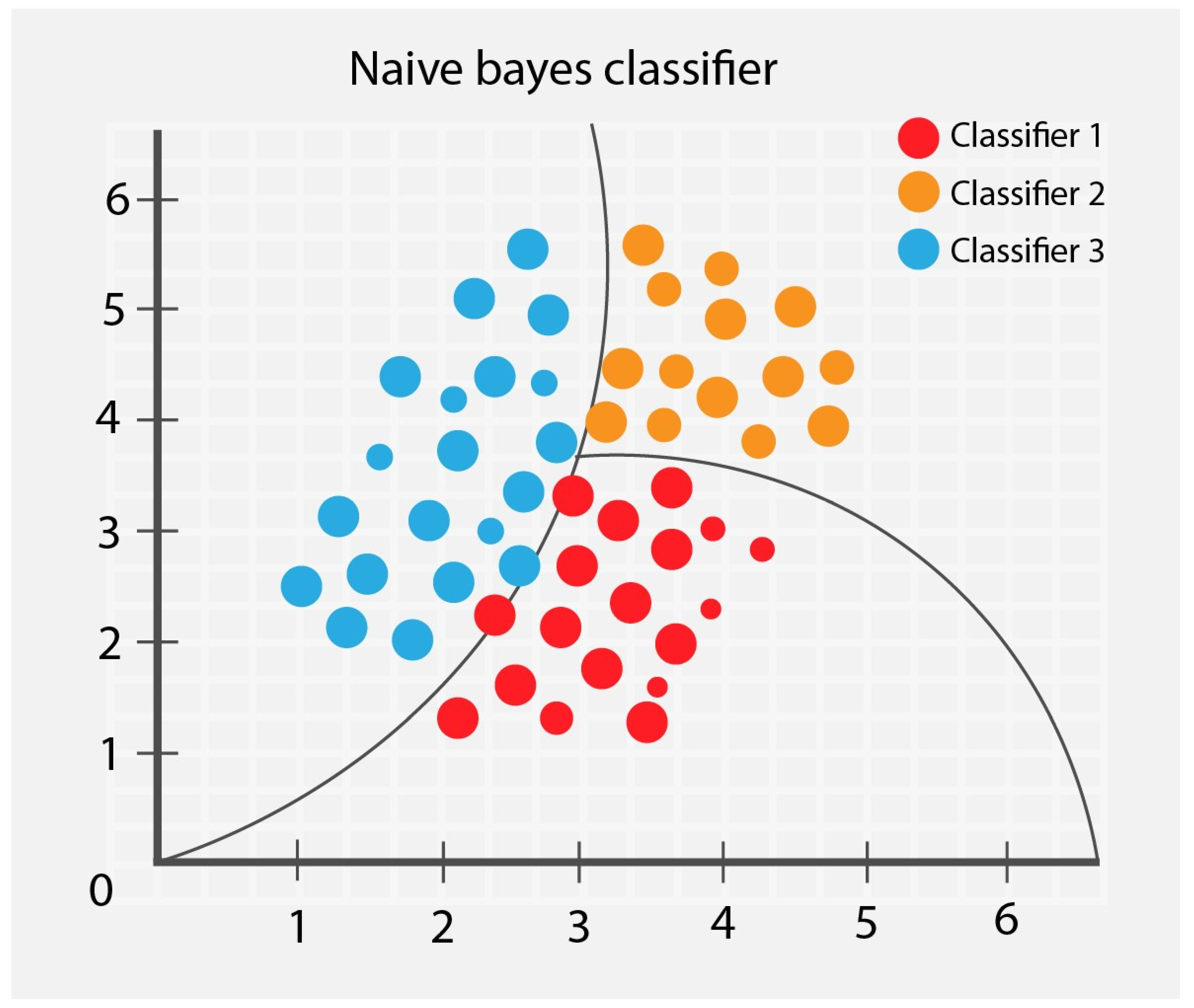
Naïve Bayes is a statistical technique based on Thomas Bayes’ theorem. According to Bayes’ theorem, it is possible to find the probability of a particular event to occur, given a chance of another that has already occurred [32]. This algorithm involves fewer computations than other algorithms because it determines the conditional input probabilities and the observed output and quickly analyzes the relationship between the input and the output. This algorithm is noticeable in the initial detection stage and can be useful in the infection’s diagnosis or harmful diseases [33]. Naïve Bayes assumes that all features are independent, which makes the algorithm fast.
In Orange, Naïve Bayes [34] is a fast and simple probabilistic classifier based on Bayes’ theorem with the feature independence assumption.
Figure 1 shows an example of a Naïve Bayes classifier.
3.1.2. Decision Tree
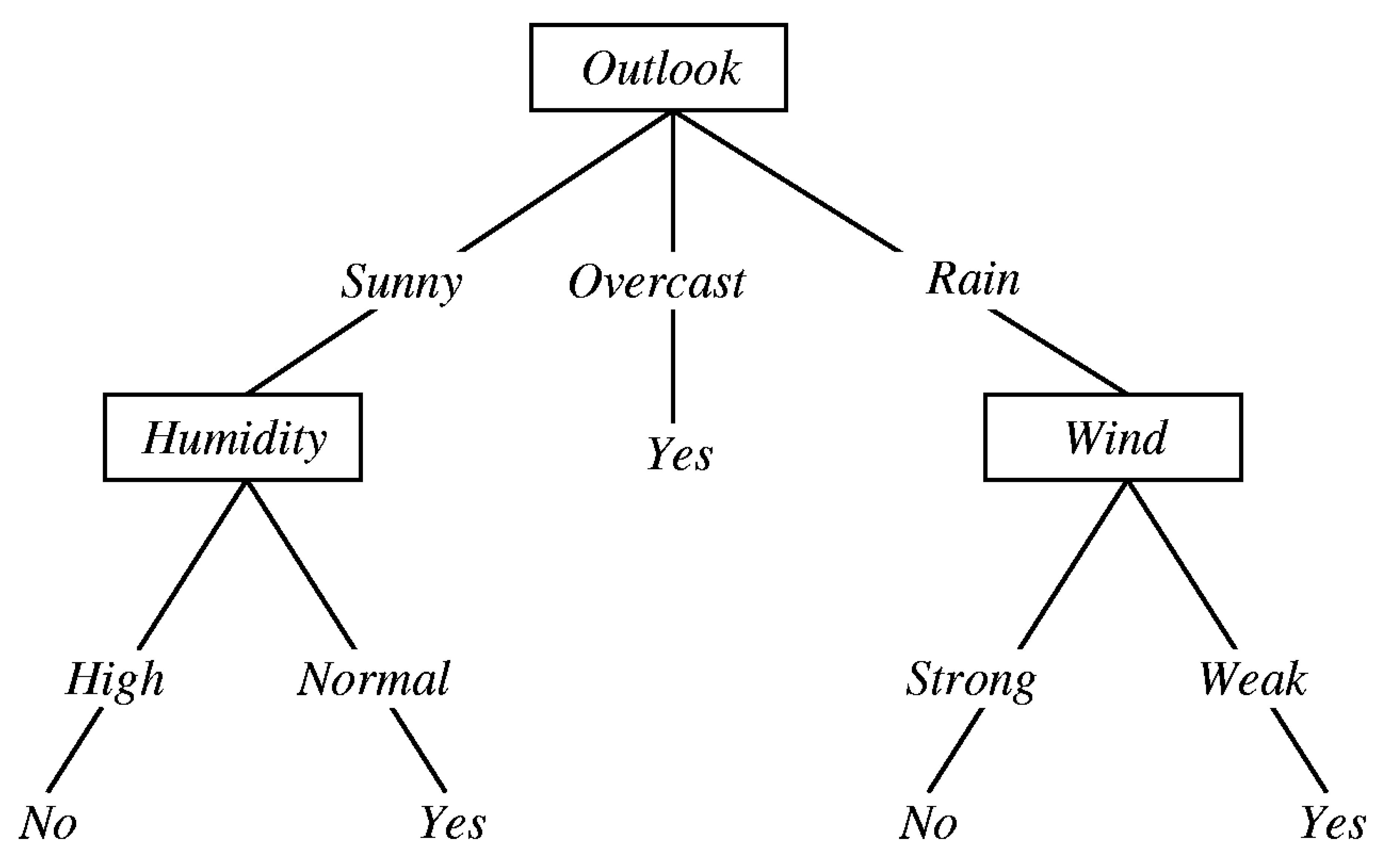
A Decision Tree is an algorithm where the nodes represent data instead of decisions. Each branch contains attributes set or classification rules associated with a particular class label, found at the branch end. These rules can be expressed in an ‘if-then’ clause, where each data value forms a clause. Each additional piece of data helps the model predict which set the subject belongs more accurately. This information can be used in a larger decision-making model [32]. The decision trees succeed since it is an effortless technique that requires no configuration parameters and usually has a good assertiveness degree. However, despite being a powerful technique, a detailed data analysis is needed to ensure good results [30].
In Orange, the Decision Tree [34] is a simple algorithm with forwarding pruning that splits the data into nodes by class purity (information gain for categorical and mean squared error (MSE) for numeric target variable). A node is 100% impure when it is split evenly 50/50 and 100% pure when all of its data belongs to a single class.
Figure 2 shows an example of an Outlook decision tree. The diagram illustrates the basic flow of the decision tree for decision making with labels (Rain (Yes), No Rain (No)).
3.1.3. Random Forest
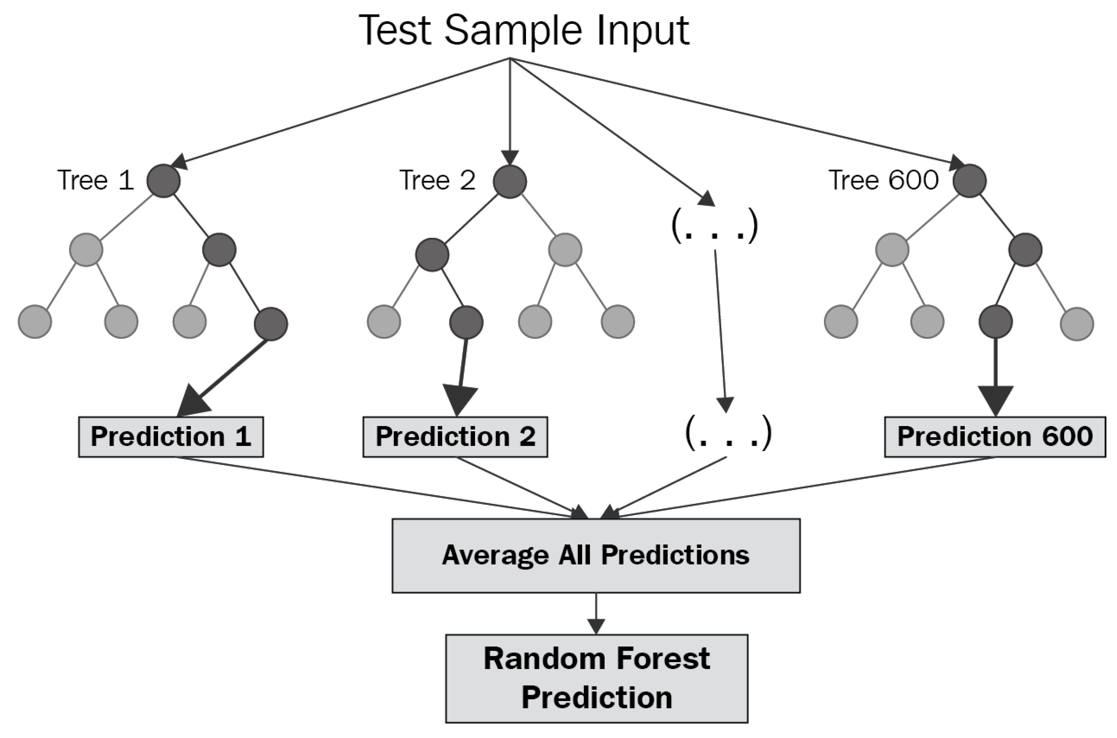
Random Forest is a supervised learning algorithm. It builds multiple decision trees and merges them to obtain a more accurate and stable prediction. Random forests are a combination of a tree or more predictors. Each tree depends on the values of a random vector sampled independently and with the same distribution for all trees in the forest [35]. One considerable advantage of the Random Forest algorithm is that it can be used for classification and regression problems, which form the most current machine learning systems.
In Orange, the Random Forest [34] prediction uses a decision trees ensemble.
Figure 3 shows an example of a random forest prediction test sample. The trees in random forests are run in parallel, and there is no interaction between these trees while building the trees. It combines the result of multiple predictions, which aggregates many decision trees.
3.1.4. Logistic Regression
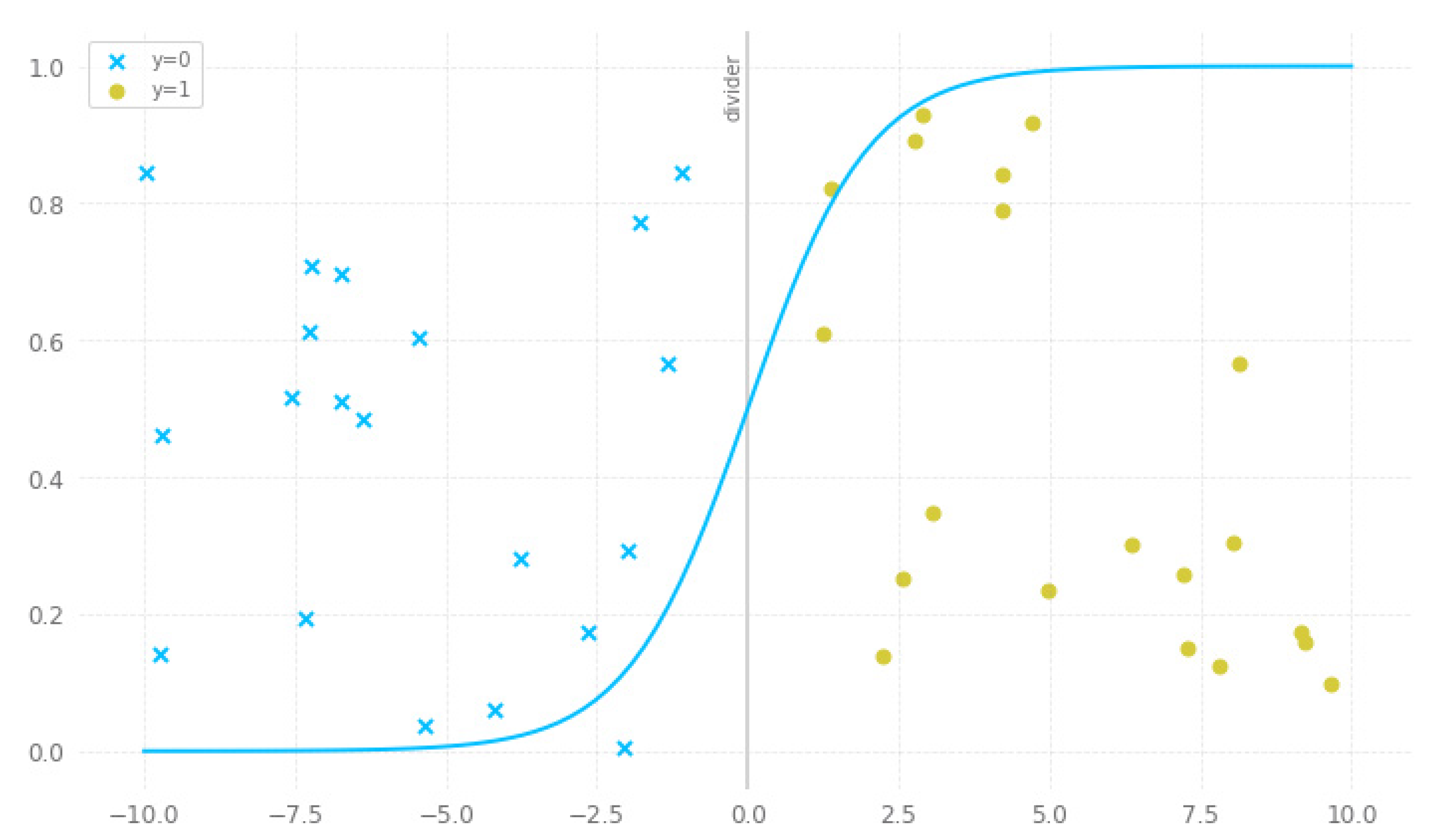
Logistic Regression is a statistical machine learning algorithm similar to linear Regression. It classifies the data by considering outcome variables on extreme ends and draws a logarithmic line that distinguishes them. Logistic regression produces a logistic curve limited between 0 and 1. The main advantage is to avoid confounding effects by analyzing the association of all variables together [36].
In Orange, the Logistic Regression [34] is a classification algorithm with LASSO (L1) or ridge (L2) regularization. The critical difference between these two is the penalty term. Ridge regression adds “square magnitude” of a coefficient as penalty term to the loss function. The experiments used ridge (L2) regularization because it is the Orange Data Mining default parameter.
Figure 4 shows an example of logistic regression. The core of logistic regression is the sigmoid function. The sigmoid function maps a continuous variable to a closed set [0, 1], which then can be interpreted as a probability. Every data point on the right-hand side is interpreted as y = 1 and every data point on the left-hand side is inferred as y = 0.
4. Data Modeling
In software engineering, data modeling is the process of creating a data model for an information system to define and organize data. It is a crucial tool to accelerate application development and extract value from data. Data modeling was needed to create our Microsoft SQL Server database in this work.
This section describes the ETL (Extraction Transformation Loading) process to load the database. ETL is a data integration type divided into three steps (extraction, transformation, and loading) used to combine different sources [37]. Usually, this process is used to construct a Data Warehouse [38], but nothing prevents it from loading data into a relational database [39].
Data Extraction
COVID-19 data were collected from different sources such as hospitals, digital publications, associations working with COVID-19, etc. All datasets collected are either CSV (comma-separated values, simple text file in which commas or other symbols separate information) or XML (extensible markup language, text files that use custom tags to describe the structure of the document) files.
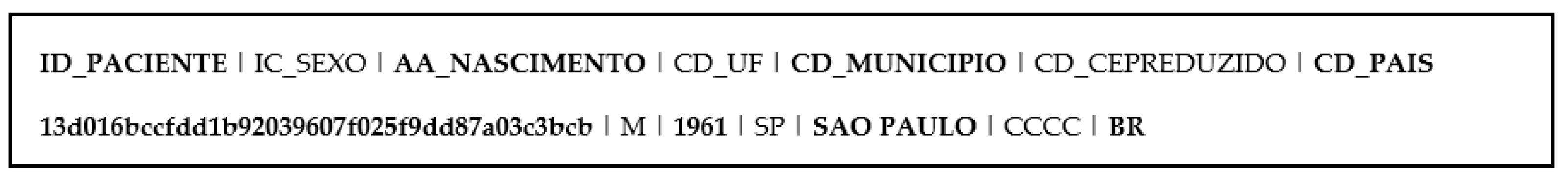
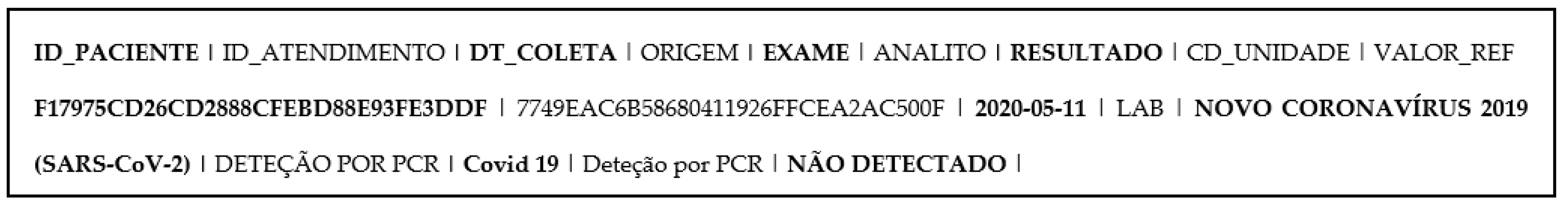
The hospital datasets possess the most significant number of records (https://repositoriodatasharingfapesp.uspdigital.usp.br/handle/item/2 (accessed on 16 July 2021)). For that reason, they were used for the SQL and NoSQL experimental tests. These data were collected from four different Brazilian hospitals who made the data available for research, namely Hospital das Clínicas da Faculdade de Medicina da Universidade de São Paulo, Grupo Fleury, Hospital Israelita Albert Einstein, and Hospital Sírio-Libanês, within the scope of the COVID-19 Data Shared Brazil project (https://fapesp.br/14956/o-repositorio-covid-19-datasharingbr-dados-abertos-no-combate-a-pandemia (accessed on 16 July 2021)). It is essential to highlight the free access to these data to develop studies such as this one, particularly when Brazil has the third highest number of positive COVID-19 cases in the world. These data have two main datasets which describe patients and exams performed by these patients. A sample of the two datasets is shown in Figure 5 and Figure 6. The patients’ dataset has 563,552 records, seven features, and its size is 30.8 MB, and the exams dataset has 26,651,926 records, nine features, and its size is 3.99 GB. These datasets gave rise to three tables, one for patients and two for exams. The first exam table, “Exame,” contains all the exams performed by the four different hospitals (it has 26,651,926 records and nine features), and the second, “ExameCovid,” includes all the exams performed to COVID-19 by the four different hospitals. It has 935,960 records and eight features. One of the features was removed because it does not have data for the COVID exams (value range feature).
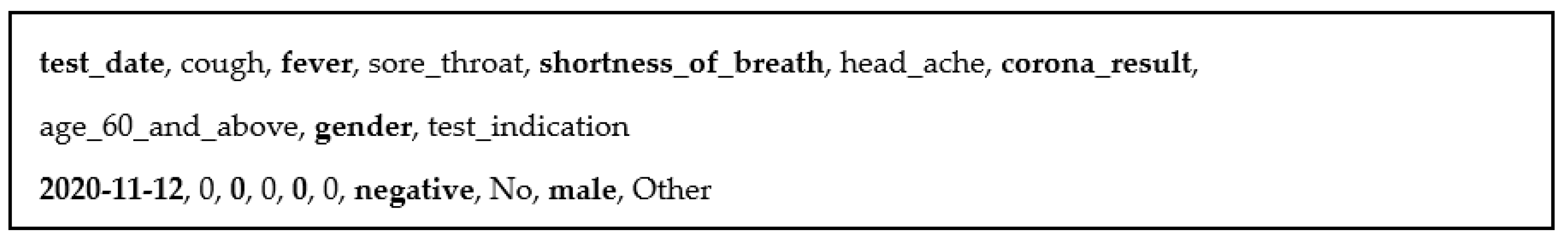
The ‘Corona tested individuals’ datasets were collected from an investigator’s GitHub (https://github.com/nshomron/covidpred (accessed on 16 July 2021)). It has two similar datasets with COVID-19 exams and patient’s symptoms: Corona tested individuals 1 has 2,742,596 records, ten features, and its size is 119 MB, and Corona tested individuals 2 has 278,848 records, ten features, and its size is 12.6 MB. The datasets include cough, fever, sore throat, shortness of breath, headache, and test results. These two datasets were put together, creating a CovidSymptoms table with 3,021,444 records and ten features. These data were used in the Data Mining classification tests because of the interesting features. A sample of the data is shown in Figure 7.
The collected datasets contain diversified information such as the number of cases, deaths, vaccinated patients, hospitalized patients, and recovered patients in several countries worldwide updated by day.
These data are spread over the tables (RegistoEuropaTeste, RegistoMundoWorldwide, RegistoMundoWho, RegistoMundoJRC, RegistoMundoOwid, RegistoUSA, RegistoVacinacaoMundoS and RegistoCasosEstimadosUSAS) of the database.
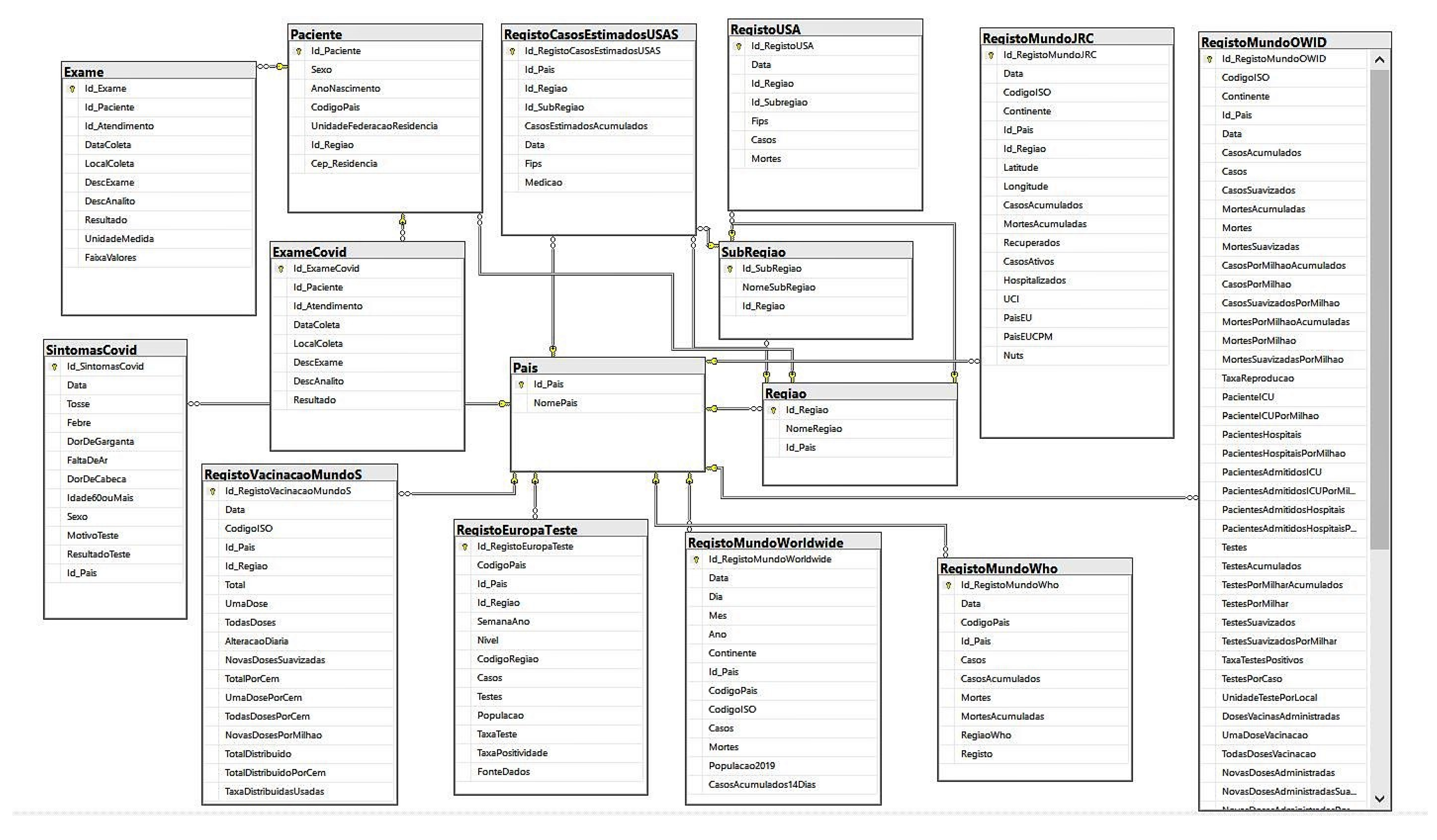
All extracted datasets were analyzed to build a relational data model where all datasets could be interconnected. This relational data model was built to create a database containing all data. The relational model was built to combine all extracted datasets, thus developing a relational model of the COVID-19 pandemic with data from different sources. As all datasets extracted had information about the country, region, or sub-region of the data in their records, three tables were created, one for Countries, one for Regions, and one for Sub-Regions (each sub-region belongs to a region and each region belongs to a country). Subsequently, through these tables, it was possible to interconnect the remaining tables (tables with data from COVID-19) and, consecutively, build the relational model, which would be used to create the database in Microsoft SQL Server. The entity-relationship model is shown in Figure 8.
Note that both MongoDB and Cassandra are NoSQL databases with different structures. MongoDB is a non-relational document-oriented database that uses collections instead of tables and documents instead of rows (records). Cassandra is a columnar non-relational database; its structure is similar to the usual relational model using tables and rows. The relational model of the COVID-19 pandemic was used to create MongoDB and Cassandra databases, with the objective of making the model of the three databases (SQL Server, MongoDB, and Cassandra) similar as possible to run the performance tests. Note that the models will never be alike because NoSQL databases use a different storage pattern than SQL databases. NoSQL databases are non-relational databases that do not need fixed table schemas and scale horizontally, thus avoiding join operations. On the other hand, SQL databases, which are relational, need relationships to store data and scale vertically, thus mostly requiring join operations.
In the case of MongoDB, the GUI (Graphical User Interface) MongoDB Compass was used to create the database, which had several collections added to it. Then, the data were imported through CSV files exported from Microsoft SQL Server to load these collections. An identical approach was taken with Cassandra using the cqlsh shell, a command-line interface to interact with Cassandra.
The final database contains 15 tables and 32,809,945 records, as illustrated above in Figure 8.
5. Experimental Evaluation
This section contains two subsections, one for Data Mining Experiments and one for Databases Experiments. The tests run on a computer with Windows 10, Intel Core i7-8750H 2.20 GHz processor, 16 GB RAM, and 256 GB SSD. SQL and NoSQL databases evaluated versions are SQL Server version 2017, MongoDB version 4.4, and Cassandra version 3.11.10.
5.1. Data Mining Experiments—Classification Tests
The Orange Data Mining platform performed all classification tests in version 3.2.9. These tests used the table SymptomsCovid because of the interesting features in it. This table has 3,021,444 records and 11 features. The features used for these tests were Gender, Age60orOlder, TestReason, Headache, Fever, Cough, SoreThroat, ShortnessOfBreath, and TestResult.
Classification tests were performed to create a suitable and helpful COVID-19 predictive model. The main goal of this model is to predict patients’ symptoms and patients’ test results based on the data features used. All these tests were performed with the cross-validation technique with ten subsets, nine for training and one for testing. Regarding the parameters of the algorithms, the default values provided by Orange Data Mining were used.
First, a precise test classification result and each patient symptom were carried out, and later the features were concatenated. Concatenation is appending one string to the end of another string.
Description of each singular classification test:
- I—Target: TestResult; 3 Possibilities: Negative (0), Positive (1), Inconclusive (2);
- II—Target: Cough; 2 Possibilities: Positive (1), Negative (0);
- III—Target: Fever; 2 Possibilities: Positive (1), Negative (0);
- IV—Target: SoreThroat; 2 Possibilities: Positive (1), Negative (0);
- V—Target: ShortnessOfBreath; 2 Possibilities: Positive (1), Negative (0);
- VI—Target: Headache; 2 Possibilities: Positive (1), Negative (0).
Description of each concatenated classification test:
- VII—Target: CoughTestResult; 6 Possibilities: Positive for cough and Negative for test result (10), Positive for both (11), Positive for cough and Inconclusive for test result (12), Negative for both (00), Negative for cough and Positive for test result (01), Negative for cough and Inconclusive for test result (02);
- VIII—Target: FeverTestResult; 6 Possibilities: Positive for fever and Negative for test result (10), Positive for both (11), Positive for fever and Inconclusive for test result (12), Negative for both (00), Negative for fever and Positive for test result (01), Negative for fever and Inconclusive for test result (02);
- IX—Target: SoreThroatTestResult; 6 Possibilities: Positive for sore throat and Negative for test result (10), Positive for both (11), Positive for sore throat and Inconclusive for test result (12), Negative for both (00), Negative for sore throat and Positive for test result (01), Negative for sore throat and Inconclusive for test result (02);
- X—Target: ShortnessOfBreathTestResult; 6 Possibilities: Positive for shortness of breath and Negative for test result (10), Positive for both (11), Positive for shortness of breath and Inconclusive for test result (12), Negative for both (00), Negative for shortness of breath and Positive for test result (01), Negative for shortness of breath and Inconclusive for test result (02);
- XI—Target: HeadacheTestResult; 6 Possibilities: Positive for headache and Negative for test result (10), Positive for both (11), Positive for headache and Inconclusive for test result (12), Negative for both (00), Negative for headache and Positive for test result (01), Negative for headache and Inconclusive for test result (02);
- XII—Target: CoughShortnessOfBreathTestResult; 12 Possibilities: Negative for all (000), Negative for cough and shortness of breath and Positive for test result (001), Negative for cough and test result and Positive for shortness of breath (010), Negative for cough and Positive for shortness of breath and test result (011), Positive for cough and Negative for shortness of breath and test result (100), Positive for cough and test result and Negative for shortness of breath (101), Positive for cough and shortness of breath and Negative for test result (110), Positive for all (111), Negative for cough and shortness of breath and Inconclusive for test result (002), Positive for cough, Negative for shortness of breath and Inconclusive for test result (102), Negative for cough, Positive for shortness of breath and Inconclusive for test result (012), Positive for cough and shortness of breath and Inconclusive for test result (112);
- XIII—Target: FeverHeadacheTestResult; 12 Possibilities: (000), (001), (010), (011), (100), (101), (110), (111), (002), (102), (012), (112);
- XIV—Target: SoreThroatShortnessOfBreathTestResult; 12 Possibilities: (000), (001), (010), (011), (100), (101), (110), (111), (002), (102), (012), (112).
Accuracy, Recall, Precision, and F1 Score were the classification evaluation metrics used in the experiments. Accuracy is the proportion of actual results among the number of the total cases examined:
where TP, FN, FP, and TN represent the number of true positives, false negatives, false positives, and true negatives, respectively.
Accuracy = (TP + TN)/(TP + FP + FN + TN)
A recall is the ratio of correctly predicted positive observations to the predicted positive observations:
Recall = TP/(TP + FN)
Precision is the ratio of correctly predicted positive observations to the total predicted positive observations:
Precision = TP/(TP + FP)
F1 Score is the weighted average of Precision and Recall:
F1 Score = 2 × (Precision × Recall)/(Precision + Recall).
Table 1, Table 2 and Table 3 show the accuracy, precision, and F1 Score results for the tests with singular targets, respectively. The Recall results were similar to the Accuracy results, and for that reason, a table was not created for Recall. The last column of all tables shows the average of the results (arithmetic mean).
In Table 1, all algorithms had outstanding accuracies. Random Forest was the best algorithm in all tests, obtaining accuracy between 99.6% when predicting breath shortness and 92.8% when predicting the COVID-19 test result. In some tests, Decision Trees has obtained the same accuracy as Random Forest (III, IV, and V) and Logistic Regression in V. The small decrease in accuracy when the COVID-19 test result is predicted since there are tests with inconclusive results. If the tests were only positive or negative, the accuracy would be higher.
In Table 2, all algorithms had remarkable precisions. Naïve Bayes was the best algorithm in four of six (III, IV, V, VI), and Random Forest was the best in 2 of 6 tests (I and II). The test with the best precision predicted breath shortness with 99.4%.
In Table 3, all algorithms had a great F1 Score and other metrics. Random Forest was the best algorithm in three of six tests (I, II, and V) and Logistic Regression (IV, V, VI). Naïve Bayes was the best in the test III. The test with the best F1 Score was when predicting breath shortness with 99.4%.
This first singular test set calculated average accuracy, precision, and F1 Score for each algorithm to select the best. The best algorithm was Random Forest, with an average accuracy of 96.88%, an average precision of 95.97%, and an average F1 Score of 96.15%. Second, Logistic Regression with an average accuracy of 96.77%, an average precision of 95.6%, and an average F1 Score of 95.87%. In third, the Decision Tree with an average accuracy of 96.60%, an average precision of 95.17%, and an average F1 Score of 95.85%. Finally, in fourth, Naïve Bayes with an average accuracy of 95.28%, an average precision of 95.73%, and an average F1 Score of 95.43%.
Table 4, Table 5 and Table 6 show the accuracy, precision, and F1 Score results for the tests with concatenated targets, respectively. It should be stated that Table 1 and Table 4 show the accuracy results. Table 2 and Table 5 show the precision results. Table 3 and Table 6 show the F1 Score results for the singular and concatenated classification tests made.
In Table 4, all algorithms show significant accuracies. The small decrease in this test is because fewer features predict more concatenated features. Despite that, the accuracy remained high. In all tests, Random Forest was the best algorithm, obtaining an accuracy between 92.4% when predicting shortness of breath combined with the test result and 89.0% when predicting the fever combined with headache and test result. Decision Trees has obtained the same accuracy as Random Forest (VII, VIII, X, XI, XII, XIII, and XIV).
In Table 5, all algorithms show good precisions. Random Forest and Decision Tree were the best algorithms in 6 of 8 tests (VII, IX, X, XI, XII, and XIV), and Naïve Bayes was the best in two of eight tests (VIII and XIII). The test with the best precision was when predicting breath shortness concatenated with a test result of 90.4%.
In Table 6, all algorithms had a good F1 Score. Random Forest and Decision Tree were the best algorithms in 6 of 8 tests (VII, IX, X, XI, XII, and XIV), and Naïve Bayes was the best in two of eight tests (VII and XII). The test with the best F1 Score was when predicting breath shortness, concatenated with a test result of 91.3%.
This second concatenated test set calculated average accuracy, precision, and F1 Score for each algorithm to select the best. The best algorithm was Random Forest, with an average accuracy of 90.68%, an average precision of 87.95%, and an average F1 Score of 89.03%. In second, Decision Tree with an average accuracy of 90.66%, an average precision of 87.95%, and an average F1 Score of 89.02%. In third, Naïve Bayes with an average accuracy of 89.91%, an average precision of 87.16%, and an average F1 Score of 88.39%. Finally, in fourth, Logistic Regression, with an average accuracy of 90.15%, an average precision of 86.40%, and an average F1 Score of 87.78%.
5.2. SQL and NoSQL Database Experiments
These experiments performed six queries on different databases (Microsoft SQL Server, MongoDB, and Cassandra). The objective was to evaluate each query’s runtime, RAM used, and CPU percentage. We also evaluated databases scalability using a dataset with a double number of records. The dataset used in these experiments was the hospital data, consisting of Patients and Exams datasets. The tests were performed for each query three times, and the final result is the average of these three executions. It should be mentioned that there exists a reset between each run to eliminate cache effects, and therefore the three executions have similar results.
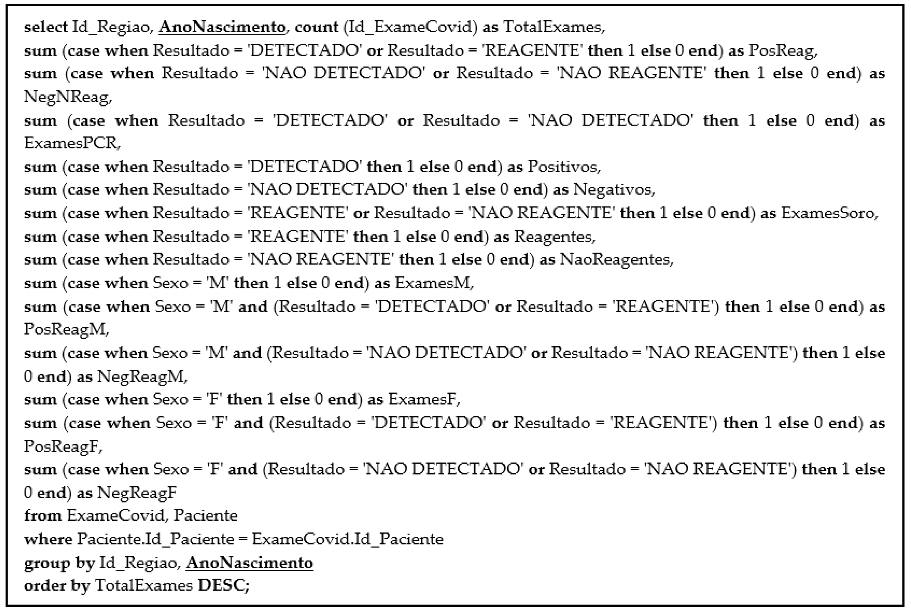
Two complex queries were created to extract valuable insights from the two tables, Patient (563,552 records) and CovidExam (935,960 records). The first query (Query Region—Query 1), in Figure 9, returns different sets of sums, excluding the underline. There are fifth sums:
- The first set is the total counts performed for COVID-19 (PCR and serological tests): how many of these tests were detected or reactive to COVID-19 and how many were not seen or not reactive COVID-19;
- The second set is the total number of PCR tests: how many of these tests were detected by COVID-19, and how many were not seen by COVID-19;
- The third set is the total number of serological tests: how many of these tests were reactive to COVID-19, and how many were non-reactive to COVID-19;
- The fourth set is the total tests performed on male patients: how many of these tests were detected or reactive to COVID-19, and how many of these tests were not seen or not reactive to COVID-19;
- Finally, the fifth set is the total tests performed on female patients: how many of these tests were not detected or not reactive to COVID-19.
All these sets are grouped by the Id of the patient’s region.
The second query (Query RegionYear—Query 2) in Figure 9 includes the underline returns the same as the first query, but it is also grouped by the patient’s birth year.
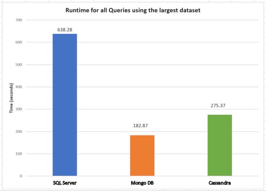
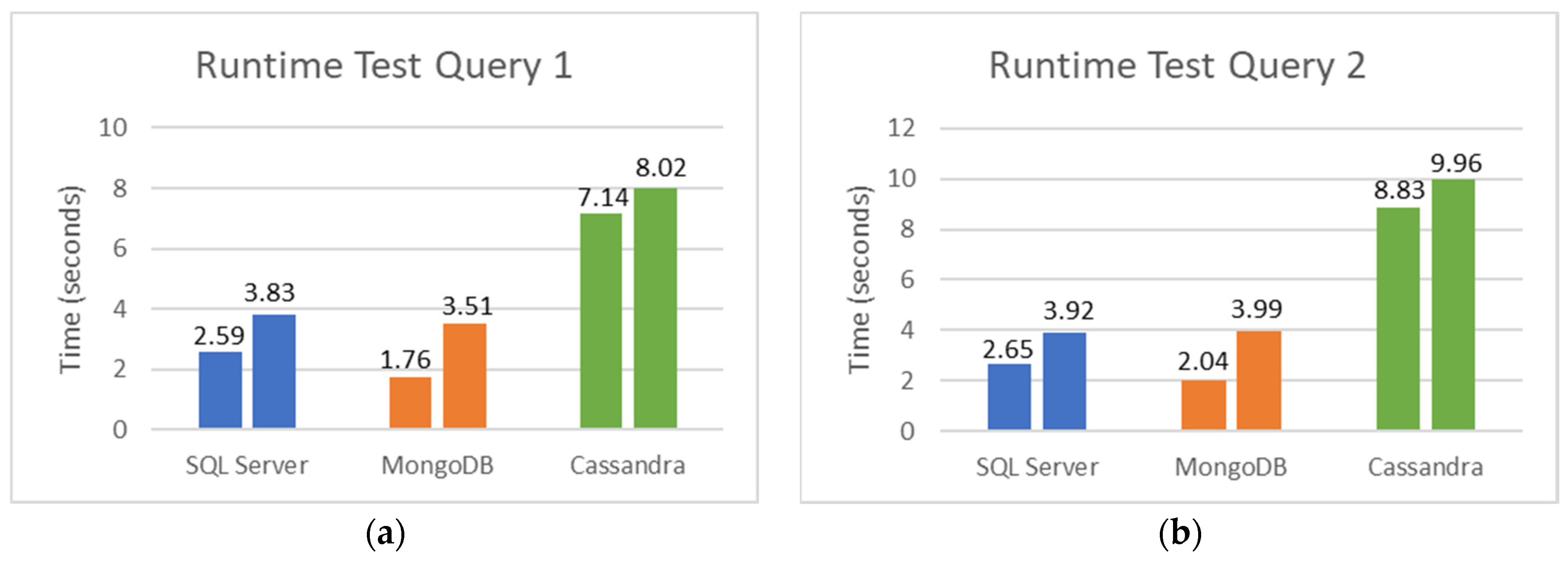
Figure 10a,b show the runtime results for Query 1 and Query 2, respectively, during their execution in different databases. The scalability was assessed using ExamCovidPatient with 467,980 records (first test) and 935,960 records (second test). Analyzing the results, the performance of MongoDB is better than Microsoft SQL Server and better than Cassandra. In this case, we use one single table (ExamCovidPatient) to avoid the join operation on NoSQL databases.
For example, using Query 1, MongoDB presents the best results (1.76 s) compared to SQL Server (2.59 s) and Cassandra (7.14 s), using the smallest dataset. The runtime of SQL Server has an overhead of 1.47 times compared to MongoDB and Cassandra shows an even worse overhead of 4.05 times. This is because MongoDB is a distributed database by default, which allows horizontal scalability without any changes to application logic.
Analyzing the database scalability when the size increases two times, we expect a linear increase in runtime. However, all the databases show good scalability, presenting an increase in the runtime of only 1.99 (MongoDB), 1.49 (SQL Server), and 1.12 (Cassandra). In this case, we can conclude that all databases perform well when we increase the workload. Query 2 results are similar with only an insignificant increase in the runtime of all databases because of added complexity.
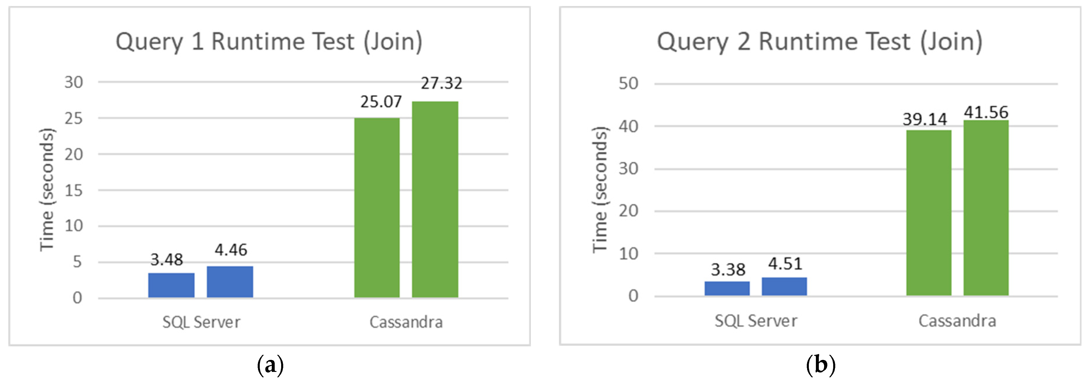
We also tested MongoDB with join queries, but it did not execute the queries in a reasonable amount of time. These tests show that MongoDB would take a very long time to execute the intended query, and further confirm that MongoDB is inadequate to join queries but performs very well in large datasets. Cassandra was connected to Apache Spark version 3.1.2. and it ran the join queries without any problems but with a significant execution time.
Figure 11a,b show the runtime results for Query 1 and Query 2, respectively, using SQL Server and Cassandra with joint operations. The runtime increases in both databases, but it is more noticeable in Cassandra because of mentioned weaknesses of NoSQL databases in these cases.
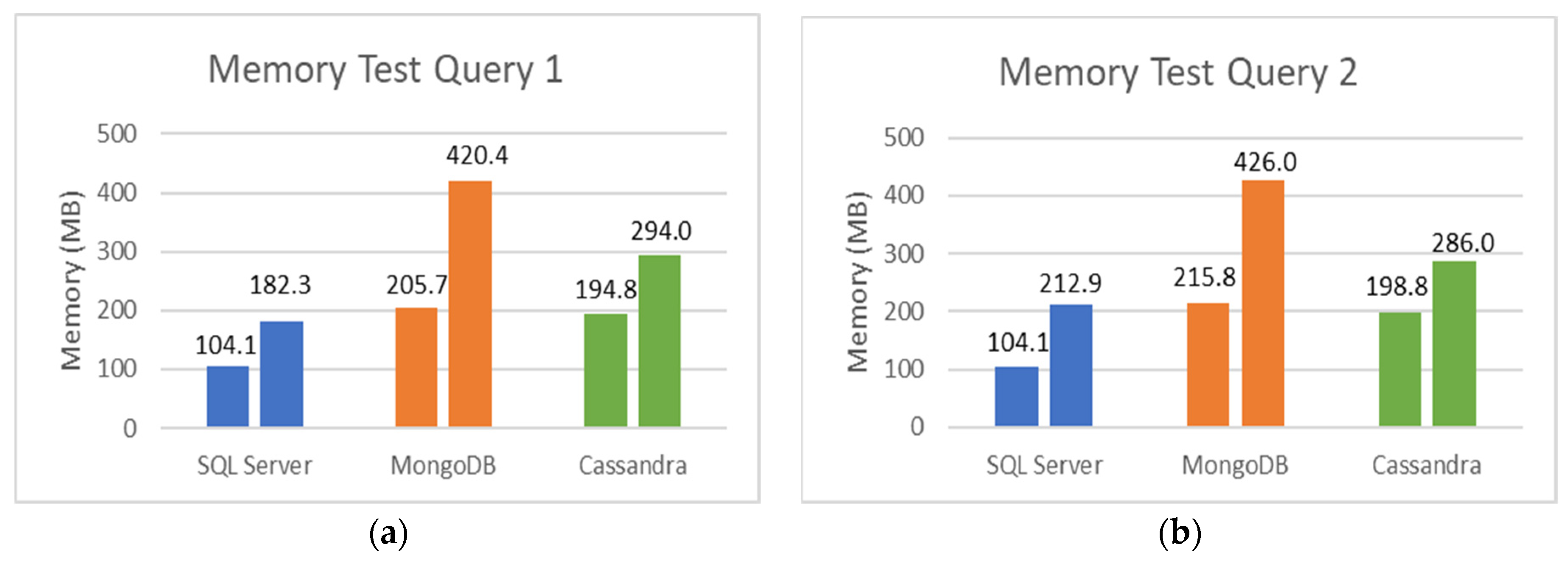
Figure 12a,b show the RAM usage for Query 1 and Query 2 during execution in different databases. Microsoft SQL Server used less memory than MongoDB and Cassandra in both queries. Using MongoDB, the difference is from a minimum of 101.6 MB to a maximum of 238.11 MB. This difference is marginal with Cassandra, where the minimum difference is 73.1, and the maximum is 111.7 MB when compared to SQL Server RAM use. This might be due to MongoDB and Cassandra’s use of data replication.
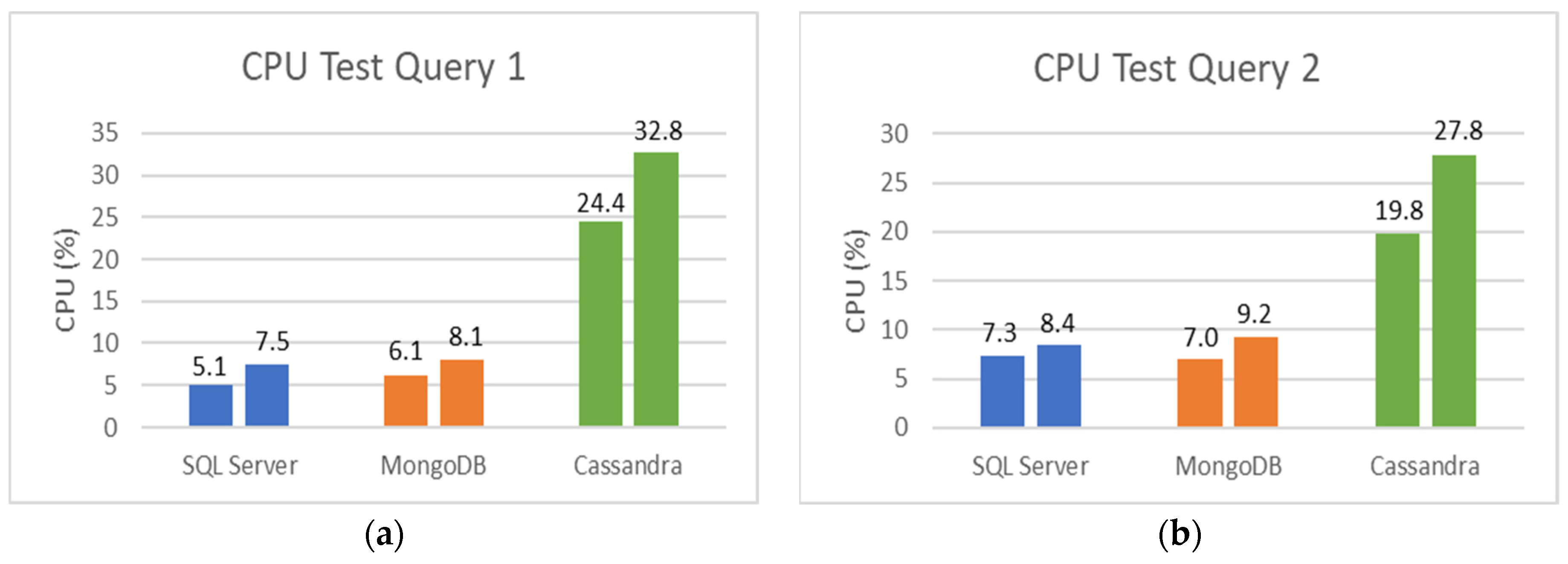
Figure 13a,b show the percentage of CPU usage results for Query 1 and Query 2, respectively, during its execution in the different databases. Microsoft SQL Server was observed to use less CPU than MongoDB and Cassandra when executing both queries with a maximum difference of 1.19× and 4.78×, respectively.
The third query (Query Orange—Query 3) was selected using an activated audit trail that controlled all the selects made in the Microsoft SQL Server database. When Orange Data Mining was connected to Microsoft SQL Server, and the Data Mining tests (classification tests) were performed, the audit trail controlled all queries that Orange needed to make in the database to perform the tests. Therefore, the third query evaluated was the query audit showed. This query, in Figure 14, outputs the number of records in table SymptomsCovid.
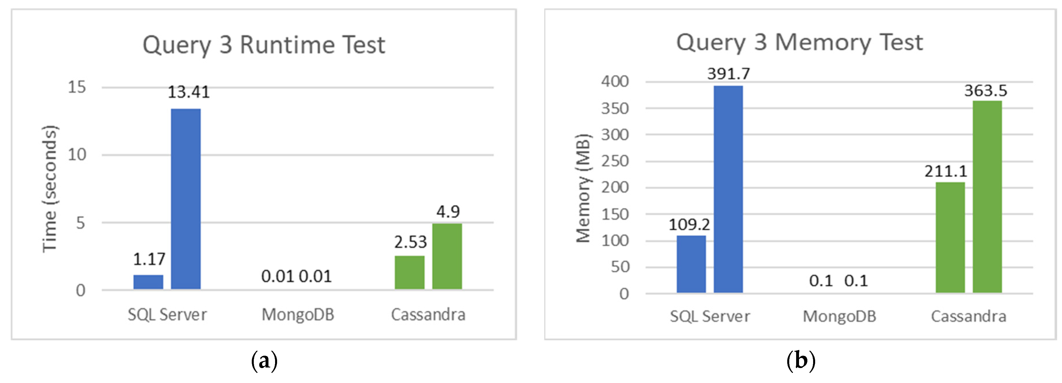
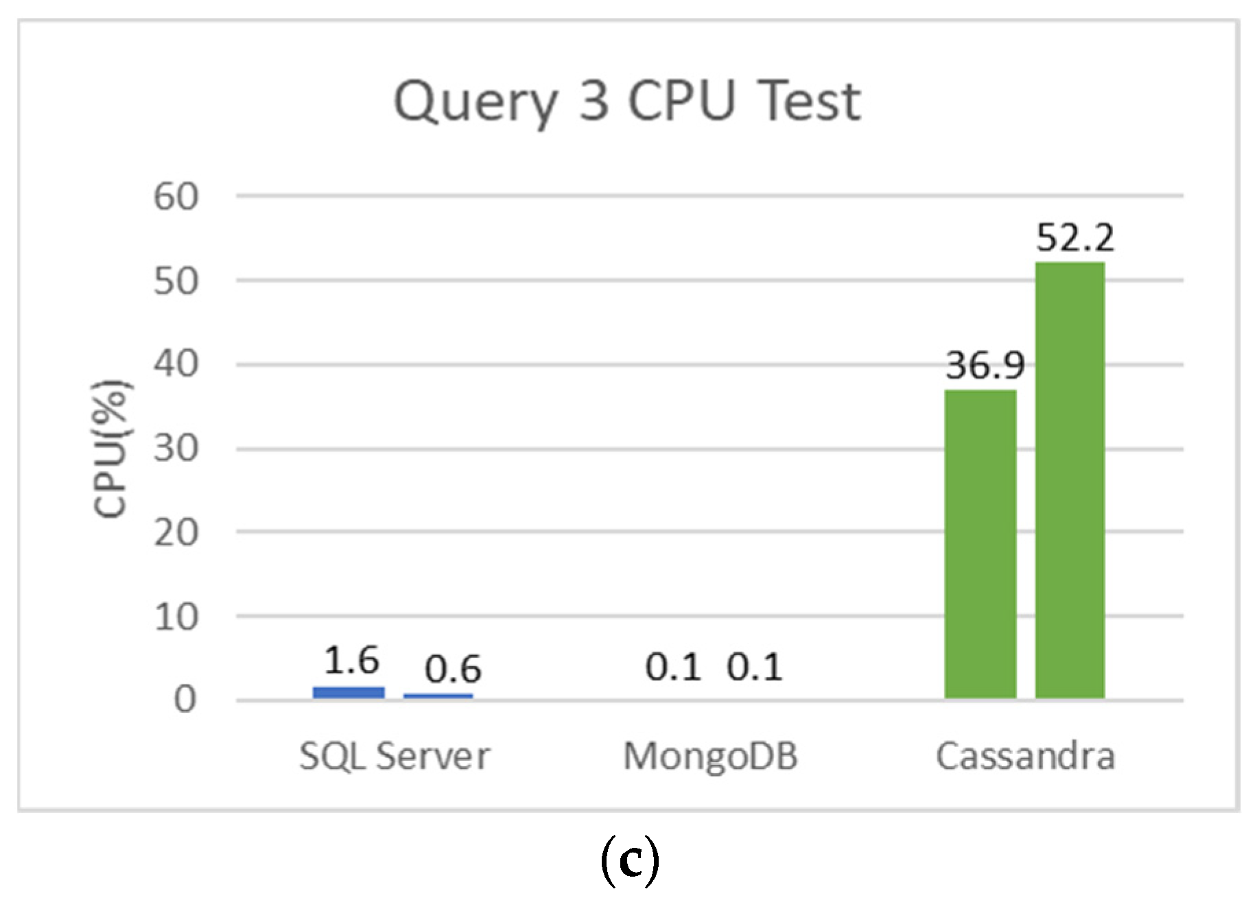
Figure 15a–c show the Query 3 results during its execution using the different databases. The scalability was assessed using SymptomsCovid with 1,510,722 records in the first test and 3,021,444 records in the second test. The results from Figure 15a show that MongoDB and Cassandra were much better than Microsoft SQL Server in runtime as expected, since NoSQL databases rely on denormalization and try to optimize for the denormalized case. This factor makes queries much faster because data are stored in the same place (table or collection), and there is no need to perform a join. The relational model used by SQL Server proves to be quite harmful to queries in databases such as Query 3. It should be noted that SQL Server presents a maximum runtime overhead of 1341× compared to MongoDB (13.41/0.01).
In Figure 15b, Microsoft SQL Server is shown to be the database that uses more memory for this query. Finally, according to Figure 15c, none of the databases used much CPU (%) to execute this query, except Cassandra.
Considering the low number of records, a new table was created and named FactosExame (joint between Paciente table and Exame table), containing 16 fields and 26,651,928 records.
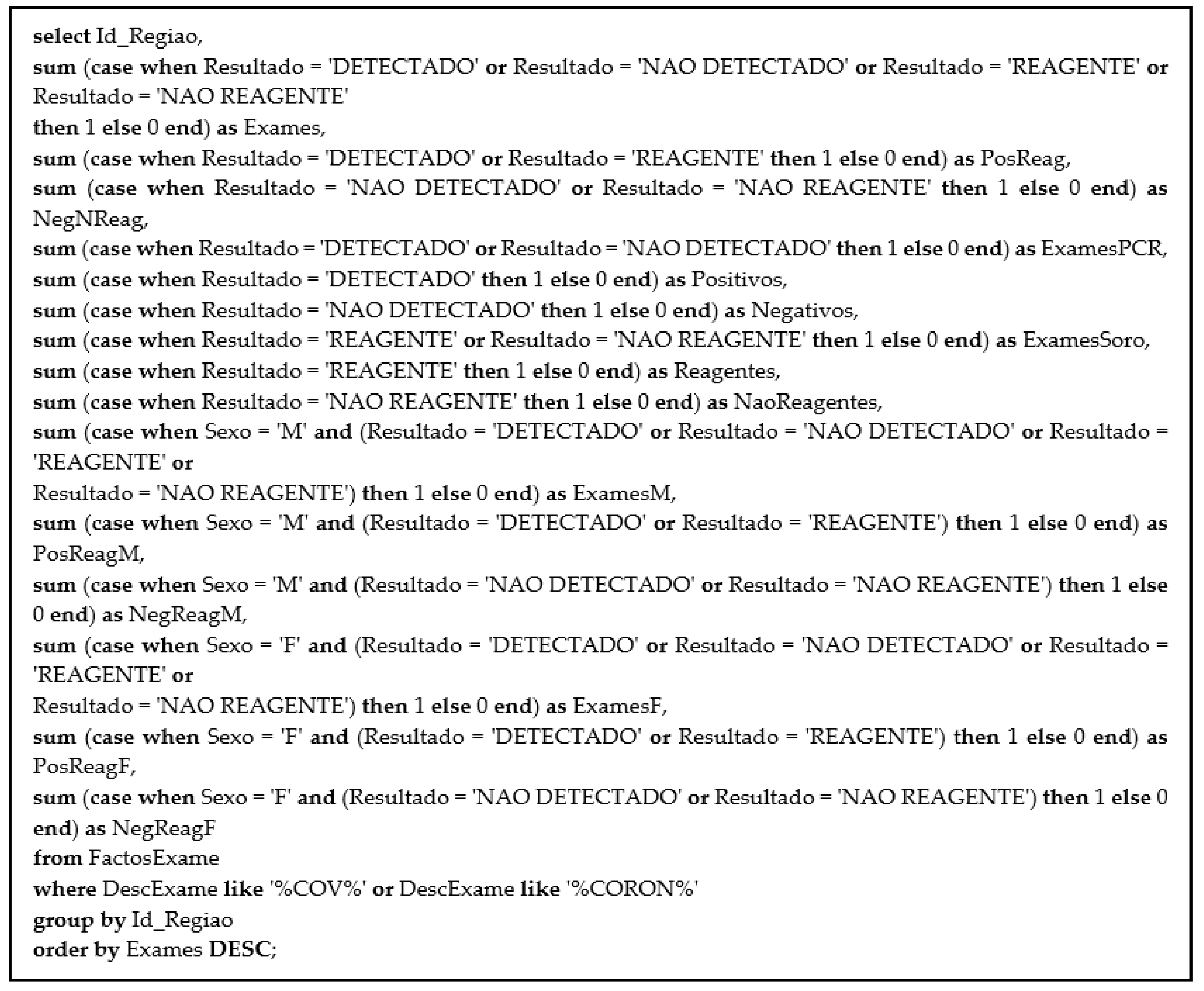
The fourth query (Query ExamFacts), in Figure 16, is very similar to the first query (Query 1). The only difference is that there is no join because the information is gathered in one table containing all the hospital exams. The scalability was assessed using FactsExam (Exam plus Patient) with 13,325,964 records (first test) and 26,651,928 records (second test).
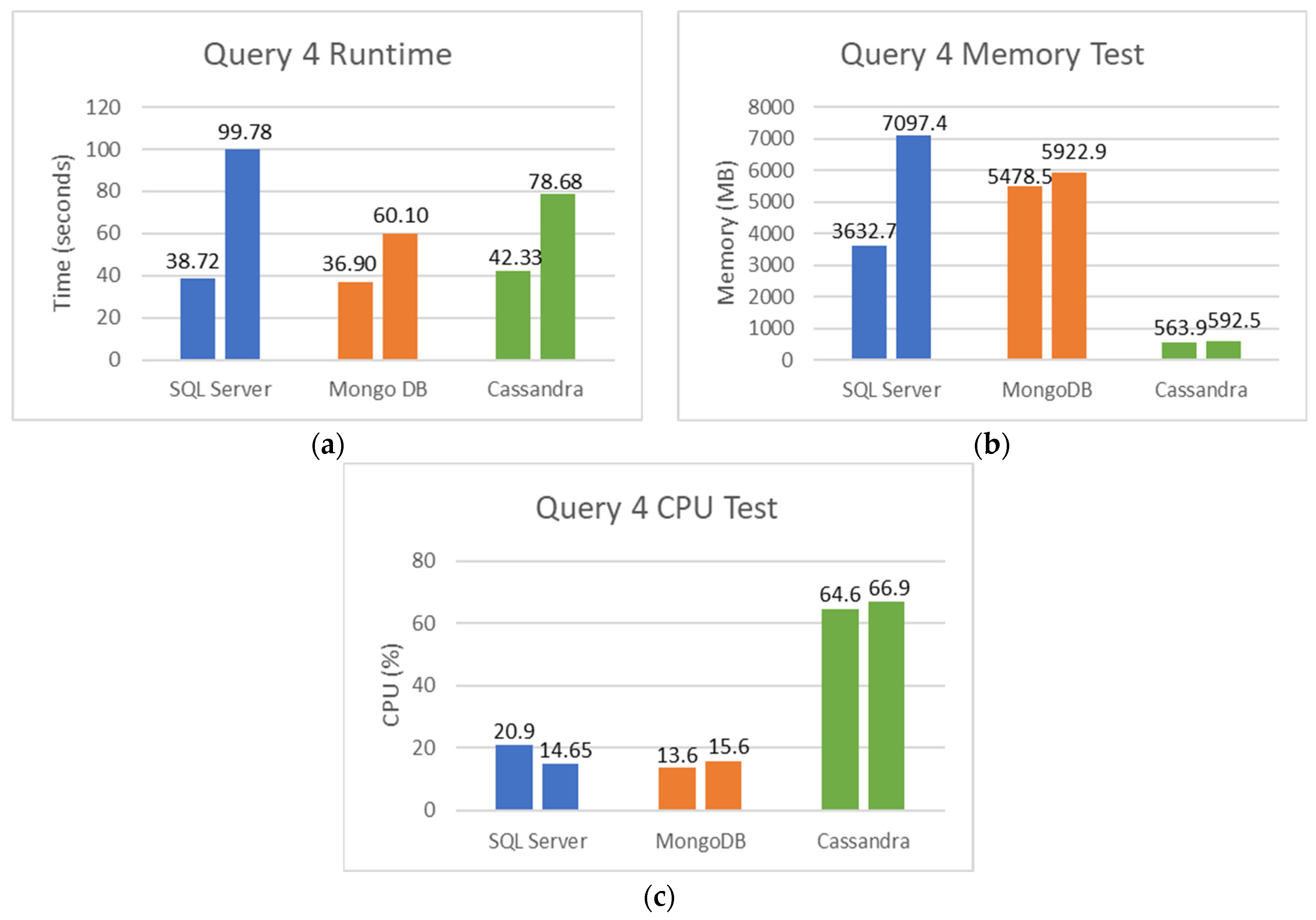
Figure 17a–c show the runtime, memory used, and CPU percentage used for the fourth query during its execution in the different databases.
The results from Figure 17a show that SQL Server was the slowest to execute the query using the most extensive dataset (1.66× quiet than MongoDB and 1.26× than Cassandra). This is due to the limitations of SQL Server working with a large amount of data. On the other hand, MongoDB was faster than Cassandra by about 18 s (i.e., 1.31× faster).
In Figure 17b, the results for the most extensive dataset show that SQL Server is the database that needed more memory to execute the query, followed by MongoDB with less than 1174.5 MB. Cassandra was by far the one that needed to use the least amount of memory, with a difference of 6504.9 MB for SQL Server and 5330.4 MB for MongoDB. SQL Server scales vertically, which means that increasing components such as RAM or CPU enable the increase of the load on a single machine. This explains the high memory values by SQL Server. MongoDB keeps all data in its caches, and it will not release them until it reaches the in-memory storage maximum threshold, which is by default 50% of physical RAM minus 1 GB. This means its memory will increase continuously when data are written or read. MongoDB will not free memory unless another process asks for it [36]. This explains the high memory values used by MongoDB.
In Figure 17c, SQL Server needs less CPU usage during the query execution for the largest dataset. Comparing the two NoSQL Databases, MongoDB used much less CPU percentage than Cassandra, separated by a difference of 4.28 times. The small CPU percentage obtained by MongoDB might be because MongoDB correctly made indexing.
Comparing the two NoSQL databases, it is possible to observe from the results in these last experiments that MongoDB was faster than Cassandra. MongoDB keeps all its data in cache memory, thus using more memory and consecutively using a lower CPU percentage. On the other hand, as Cassandra uses little memory, it does not keep its data in the cache, thus needing to use high values of CPU percentage to complete the execution of the query. For this reason, Cassandra is a bit slower when running the query.
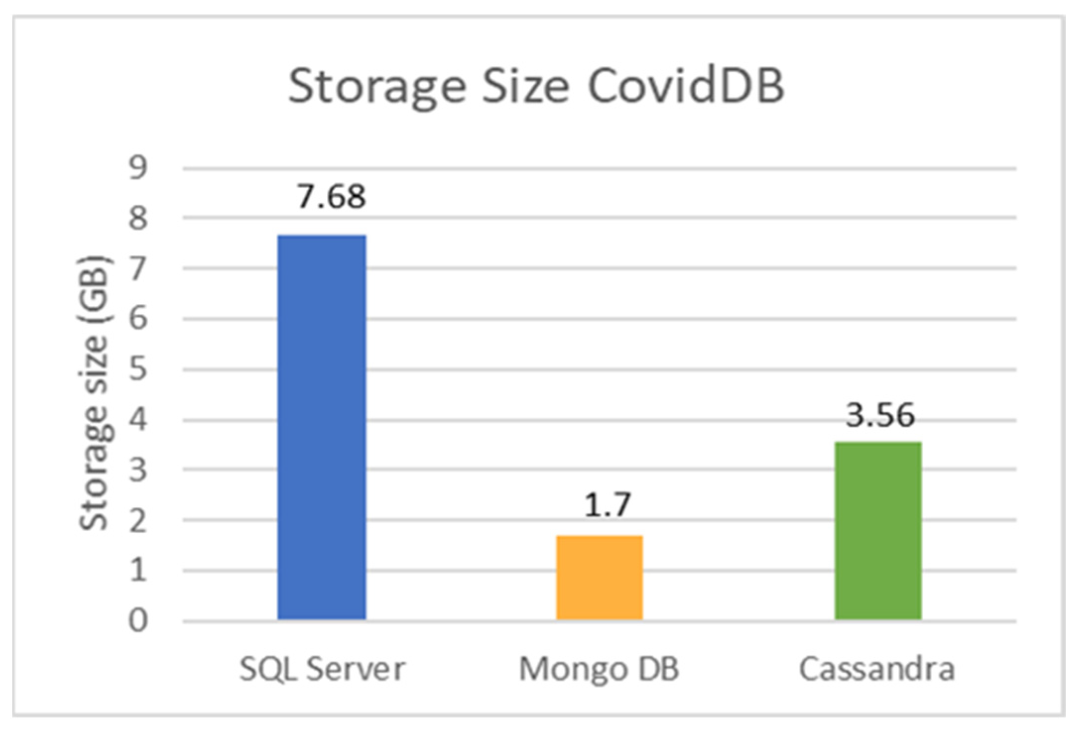
We also evaluate the storage size of each database when storing the most extensive dataset, and the results are illustrated in Figure 18. This figure shows that MongoDB was the best performing solution, followed by Cassandra and, lastly, Microsoft SQL Server (more 4.51× than MongoDB and 2.16× than Cassandra). MongoDB’s better performance is due to the WiredTiger storage engine that compresses data and indexes by default. Otherwise, the storage would be more significant.
We are interested in testing the databases with more complex queries that need more processing power. Therefore, we define two more queries: Query 5 and Query 6.
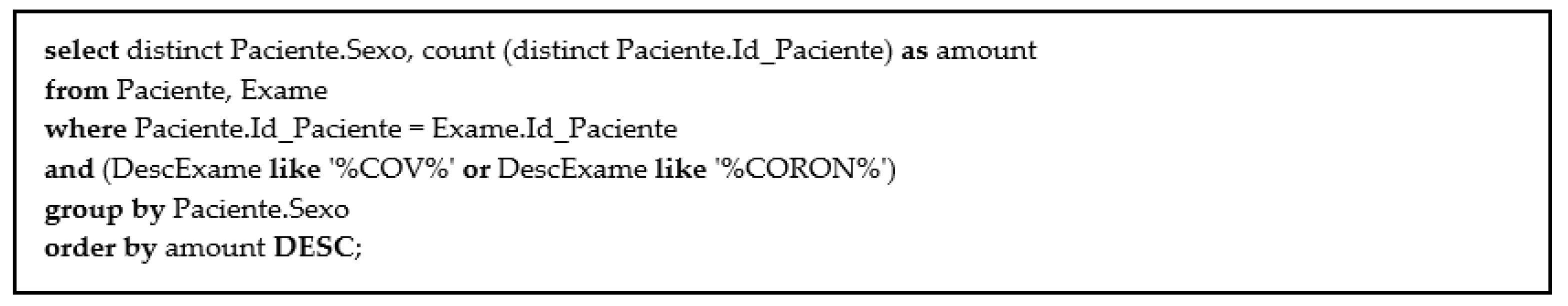
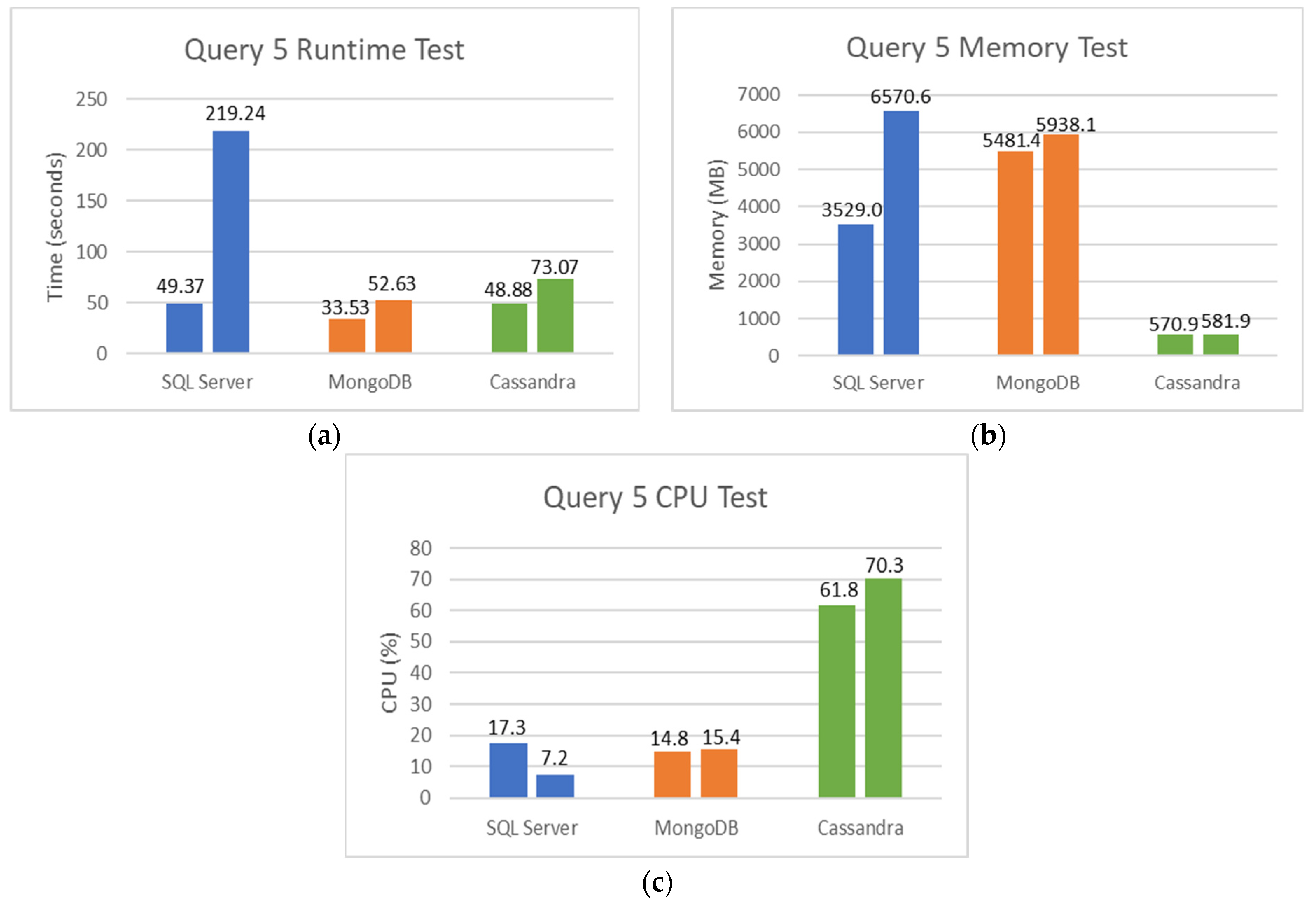
Query 5 is shown in Figure 19 and returns the number of female and male patients who underwent COVID tests, which corresponds to only two rows.
Figure 20a–c show the runtime, memory used, and CPU percentage used for the fifth query using the different databases. The first test uses an Exam table with 13,325,964 records and the second one with 26,651,928 records.
Figure 20a shows the superior runtime of MongoDB: 4.16× better than SQL Server and 1.49× than Cassandra. Analyzing the scalability of each database when the number of records is duplicated, SQL Server shows an increment of 4.44×, MongoDB 1.56×, and Cassandra 1.49×. These results demonstrate the superior performance of NoSQL databases when dealing with large datasets.
The results for RAM and CPU usage are consistent with the previous test and show that Cassandra is the best in using RAM memory, and MongoDB uses less CPU.
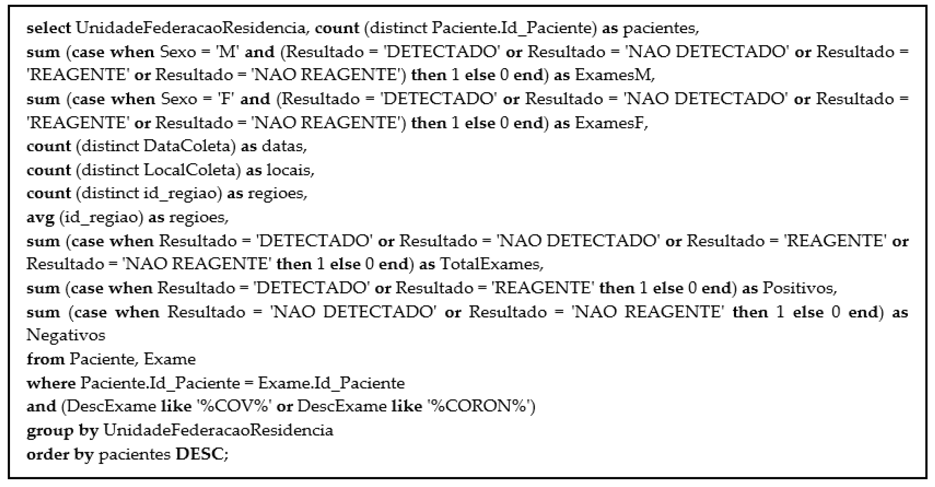
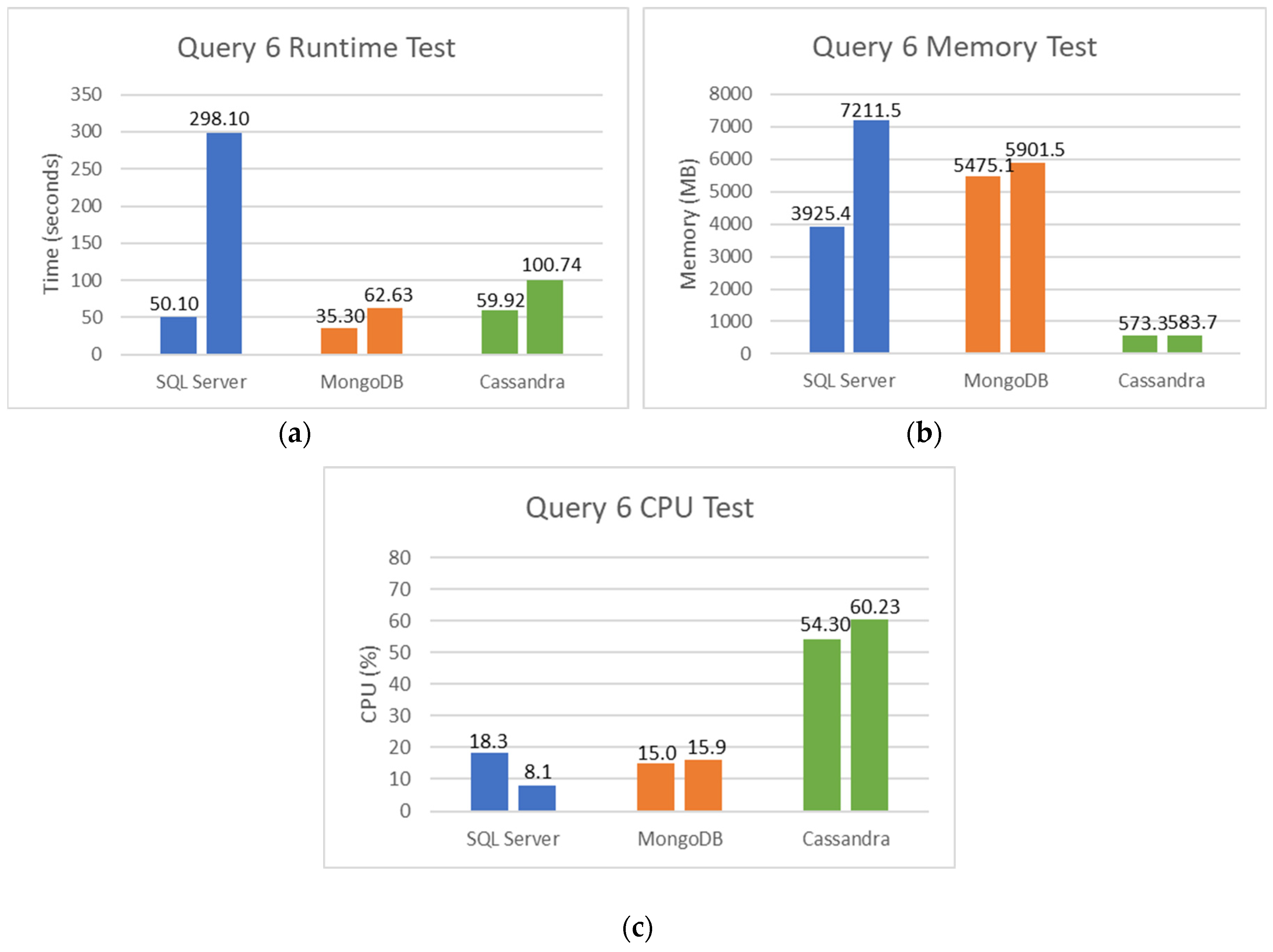
Query 6 is shown in Figure 21 and returns 21 rows with the federation unity of each state that underwent COVID tests. Each row has the number of female and male patients who underwent COVID tests, the number of different sample collection dates, the number of other sample collection locations, the number of different regions, the most present region, and the total counts performed for COVID-19 (PCR and serological tests), how many of these tests were detected or reactive to COVID-19 and how many were not detected or not reactive COVID-19. This is the most challenging query used in the experiments.
Figure 22a–c show the runtime, memory used, and CPU percentage used for the sixth query, where the first test uses an Exam table with 13,325,964 records and the second one 26,651,928 records.
Figure 22a shows better results than Query 5, with MongoDB achieving a runtime 4.75× better than SQL Server and 1.60× than Cassandra. Analyzing the scalability of each database when the number of records is duplicated, SQL Server shows an increment of 5.95×, MongoDB 1.77×, and Cassandra 1.68×.
The results for RAM and CPU usage are also consistent with the previous tests and show that Cassandra continues to be the best in the use of RAM and MongoDB in the utilization of CPU.
In summary, MongoDB and Cassandra are databases that do not require a schema, naturally making them more adaptable to changes.
Cassandra is a much more stationary database. It facilitates static typing and demands the categorization and definition of columns beforehand, requiring much less RAM. Additionally, the load characteristic of the application database to support also plays a crucial role. If we are expecting heavy load input, Cassandra will provide better results with its multiple master nodes. With stout load output, both MongoDB and Cassandra will show good performance.
Finally, many consider MongoDB or SQL Server to have the upper hand regarding consistency requirements. Ultimately, the decision between these three databases will depend on the application requirements and model.
6. Conclusions and Future Work
The COVID-19 pandemic has impacted millions of lives worldwide as a significant public health concern. Therefore, we all need to work together to end it and return to normality. In this study, a COVID-19 database was created and used for Data Mining on some of those data.
The COVID-19 predictive model obtained good accuracy in the classification tests with all the algorithms used. The best algorithm was Random Forest with an average accuracy of 96.88%, recall of 96.88%, precision of 95.97%, and F1 Score of 96.15% in particular target classification. Similarly, concatenated target classification obtained an average accuracy of 90.68%, recall of 90.68%, precision of 87.95%, and F1 Score of 89.03%. Consequently, this predictive model proved an asset in the fight against COVID-19 as a result of its high accuracy.
Regarding the second objective of this project—determining the most appropriate database to store COVID-19 data, with the actual characteristics—SQL Server should be the choice if the data are very structured and needs to join queries. Cassandra and MongoDB showed worse performance with joint queries.
Nevertheless, if a large unstructured data volume is used and there is no need to perform join queries, MongoDB or Cassandra are considered the most appropriate solutions. For the queries used, MongoDB was faster, and used less CPU percentage and storage size than Cassandra. On the other hand, Cassandra was the best in terms of memory usage. Ultimately, our choice would be MongoDB. Analyzing the scalability, the NoSQL databases show superior performance than the SQL Server, demonstrating that they are more appropriate for processing large amounts of data.
As future work, we intend to extend the database model to provide more significant results that could help in the current pandemic situation and future similar cases. Studies of this kind must continue to be developed to respond to the needs and demands that a pandemic may cause. Predictive models can be an asset to medicine, so there is an ambition to continue building great models and testing new Machine Learning algorithms. We also intend to verify whether ontologies can improve the classification process, memory consumption, and query performance.
Author Contributions
Conceptualization, R.R.S. and J.B.; Methodology, J.A. and R.R.S.; Software, J.A.; Validation, J.A., R.R.S. and J.B.; Formal analysis, J.A., R.R.S. and J.B.; Investigation, J.A.; Resources, J.A.; Data curation, J.A.; Writing—original draft preparation, J.A., J.B. and R.R.S.; Writing—review and editing, J.A., J.B. and R.R.S.; Supervision, J.B. and R.R.S.; Project administration, R.R.S. and J.B.; Funding acquisition, J.B. All authors have read and agreed to the published version of the manuscript.
Funding
This research received no external funding.
Institutional Review Board Statement
Not applicable.
Informed Consent Statement
Not applicable.
Data Availability Statement
The datasets used in the experiments are publicly available at the following links: 1. Dataset Hospital https://repositoriodatasharingfapesp.uspdigital.usp.br/handle/item/2 (accessed on 1 April 2021); 2. Dataset Corona tested individuals https://github.com/nshomron/covidpred (accessed on 1 April 2021). The datasets not used in the experiments, but used to create the COVID-19 database are publicly available at the following links: 3. Dataset Our World in Data https://github.com/owid/covid-19-data/tree/master/public/data (accessed on 1 April 2021); 4. Dataset Our World in Data Testing https://github.com/owid/covid-19-data/tree/master/public/data/testing (accessed on 1 April 2021); 5. Dataset COVID-19 geographic distribution worldwide https://www.ecdc.europa.eu/en/publications-data/download-todays-data-geographic-distribution-covid-19-cases-worldwide (accessed on 1 April 2021); 6. Dataset Vaccinations https://github.com/owid/covid-19-data/tree/master/public/data/vaccinations (accessed on 1 April 2021); 7. Dataset WHO COVID-19 Global Data https://data.humdata.org/dataset/coronavirus-covid-19-cases-and-deaths (accessed on 1 April 2021); 8. Dataset FAIR COVID-19 US County https://data.humdata.org/dataset/fair-covid-dataset (accessed on 1 April 2021), 9. Dataset JRC Data https://github.com/ec-jrc/COVID-19 (accessed on 1 April 2021).
Conflicts of Interest
The authors declare no conflict of interest. The funders had no role in the design of the study; in the collection, analyses, or interpretation of data; in the writing of the manuscript, or in the decision to publish the results.
References
- Samal, J. A Historical Exploration of Pandemics of Some Selected Diseases in the World. IJHSR 2014, 4, 165–169. [Google Scholar]
- Shi, H.; Han, X.; Jiang, N.; Cao, Y.; Alwalid, O.; Gu, J.; Fant, Y.; Zhengt, C. Radiological findings from 81 patients with COVID-19 pneumonia in Wuhan, China: A descriptive study. Lancet Infect. Dis. 2020, 20, 425–434. [Google Scholar] [CrossRef]
- World Health Organization. Corona disease 2019 (COVID-19) Situation Report—No. 67; WHO: Geneva, Switzerland, 2021. [Google Scholar]
- Leshem, E.; Wilder-Smith, A. COVID-19 Vaccine Impact in Israel and a Way Out of the Pandemic; Elsevier: Amsterdam, The Netherlands, 2021; Volume 397, pp. 1783–1785. [Google Scholar]
- Muhammad, L.J.; Islam, M.M.; Usman, S.S.; Ayon, S.I. Predictive data mining models for novel coronavirus (COVID-19) infected patients’ recovery. SN Comput. Sci. 2020, 1, 206. [Google Scholar] [CrossRef] [PubMed]
- Rohini, M.; Naveena, K.R.; Jothipriya, G.; Kameshwaran, S.; Jagadeeswari, M. A Comparative Approach to Predict Corona Virus Using Machine Learning. In Proceedings of the International Conference on Artificial Intelligence and Smart Systems (ICAIS), Coimbatore, India, 25–27 March 2021; pp. 331–337. [Google Scholar]
- Taranu, I. Data mining in healthcare: Decision making and precision. Database Syst. J. 2015, VI, 33–40. [Google Scholar]
- Orange Data Mining. Available online: https://orangedatamining.com (accessed on 1 September 2021).
- Abramova, V.; Bernardino, J.; Furtado, P. SQL or NoSQL? Performance and scalability evaluation. Int. J. Bus. Process. Integr. Manag. 2015, 7, 314–321. [Google Scholar] [CrossRef]
- Li, Y.; Manoharan, S. A performance comparison of SQL and NoSQL databases. In Proceedings of the IEEE Pacific Rim Conference, Conference on Communications and Signal Processing (PACRIM), Victoria, BC, Canada, 27–29 August 2013. [Google Scholar]
- Microsoft SQL Server 2017. Available online: https://www.microsoft.com/en-au/sql-server/sql-server-2017 (accessed on 1 September 2021).
- Mongo, D.B. Available online: https://www.mongodb.com/ (accessed on 1 September 2021).
- Cassandra. Available online: https://cassandra.apache.org/ (accessed on 1 September 2021).
- Nayak, A.; Poriya, A.; Poojary, D. Type of nosql databases and its comparison with relational databases. Int. J. Appl. Inf. Syst. (IJAIS) 2013, 5, 16–19. [Google Scholar]
- Mohamed, M.A.; Altrafi, O.G.; Ismail, M.O. Relational vs NoSQL Databases: A Survey. Int. J. Comput. Inf. Technol. 2014, 3, 598–601. [Google Scholar]
- Raut, D.A.B. NoSQL Database and Its Comparison with RDBMS. Int. J. Comput. Intell. Res. 2015, 7, 314–321. [Google Scholar]
- Chakraborty, S.; Paul, S.; Hasan, K.M.A. Performance Comparison for Data Retrieval from NoSQL and SQL Databases: A Case Study for COVID-19 Genome Sequence Dataset. In Proceedings of the International Conference on Robotics, Electrical and Signal Processing Techniques (ICREST), Dhaka, Bangladesh, 5–7 January 2021; pp. 324–328. [Google Scholar]
- Abramova, V.; Bernardino, J. NoSQL Databases: MongoDB vs Cassandra. In Proceedings of the C3S2E Proceedings of the International Conference on Computer Science and Software Engineering, Porto, Portugal, 10–12 July 2013; Association for Computing Machinery: New York, NY, USA, 2013. [Google Scholar]
- Abramova, V.; Bernardino, J.; Furtado, P. Which NoSQL Database? A Performance Overview. Open J. Databases (OJDB) 2014, 1, 17–24. [Google Scholar]
- Abramova, V.; Bernardino, J.; Furtado, P. Experimental evaluation of NoSQL databases. Int. J. Database Manag. Syst. 2014, 6, 1. [Google Scholar] [CrossRef]
- Lourenço, J.; Abramova, V.; Vieira, M.; Cabral, B.; Bernardino, J. NoSQL Databases: A Software Engineering Perspective. In New Contributions in Information Systems and Technologies Advances in Intelligent Systems and Computing; Springer: Berlin/Heidelberg, Germany, 2015; Volume 353, pp. 741–750. [Google Scholar]
- Muhammad, L.J.; Ebrahem, A.A.; Usman, S.S.; Abdulkadir, A.; Chakraborty, C.; Mohammed, I.A. Supervised Machine Learning Models for Prediction of COVID-19 Infection using Epidemiology Dataset. SN Comput. Sci. 2021, 2, 11. [Google Scholar] [CrossRef] [PubMed]
- Awadh, W.A.; Alasady, A.S.; Mustafa, H.I. Predictions of COVID-19 Spread by Using Supervised Data Mining Techniques. J. Phys. Conf. Ser. 2020, 1879, 022081. [Google Scholar] [CrossRef]
- Abdulkareem, N.M.; Abdulazeez, D.Q.; Zeebaree, D.A.H. COVID-19 World Vaccination Progress Using Machine Learning Classification Algorithms. Qubahan Acad. J. 2021, 1, 100–105. [Google Scholar] [CrossRef]
- Guzmán-Torres, J.A.; Alonso-Guzmán, E.M.; Domínguez-Mota, F.J.; Tinoco-Guerrero, G. Estimation of the Main Conditions in (SARS-CoV-2) COVID-19 Patients That Increase the Risk of Death Using Machine Learning, the Case of Mexico; Elsevier: Amsterdam, The Netherlands, 2021; Volume 27. [Google Scholar]
- Shanbehzadeh, M.; Orooji, A.; Arpanahi, H.K. Comparing of Data Mining Techniques for Predicting In-Hospital Mortality among Patients with COVID-19. J. Biostat. Epidemiol. 2021, 7, 154–169. [Google Scholar] [CrossRef]
- Keshavarzi, A. Coronavirus Infectious Disease (COVID-19) Modeling: Evidence of Geographical Signals. SSRN Electron. J. 2020. [CrossRef]
- Saire, J.E.C. Data Mining Approach to Analyze Covid-19 Dataset of Brazilian Patients. medRxiv 2020. [CrossRef]
- Thange, U.; Shukla, V.K.; Punhani, R. Analyzing COVID-19 Dataset through Data Mining Tool “Orange”. In Proceedings of the International Conference on Computation, Automation and Knowledge Management (ICCAKM), Dubai, United Arab Emirates, 19–21 January 2021; pp. 198–203. [Google Scholar]
- Bramer, M. Principles of Data Mining; Springer: London, UK, 2007. [Google Scholar]
- Fayyad, U.; Shapiro, G.P.; Smyth, P. From Data Mining to Knowledge Discover in Databases. AI Mag. 1996, 17, 37–54. [Google Scholar]
- Han, J.; Kamber, M.; Pei, J. Data Mining Concepts and Techniques, 3rd ed.; Elsevier: Waltham, MA, USA, 2006. [Google Scholar]
- Orange Data Mining Models. Available online: https://orange3.readthedocs.io/projects/orange-visual-programming/en/latest/index.html# (accessed on 1 September 2021).
- Joseph, S.I.T. Survey of data mining algorithms for intelligent computing system. J. Trends Comput. Sci. Smart Technol. (TCSST) 2019, 1, 14–23. [Google Scholar]
- Breiman, L. Random Forests. Mach. Learn. 2001, 45, 5–32. [Google Scholar] [CrossRef] [Green Version]
- Sperandei, S. Understanding logistic Regression analysis. Biochem. Med. 2014, 24, 12–18. [Google Scholar] [CrossRef] [PubMed]
- Bernardino, J.; Madeira, H. Experimental evaluation of a new distributed partitioning technique for data warehouses. In Proceedings of the 2001 International Database Engineering and Applications Symposium, Grenoble, France, 16–18 July 2001; pp. 312–321. [Google Scholar] [CrossRef]
- Bernardino, J.; Furtado, P.; Madeira, H. DWS-AQA: A cost effective approach for very large data warehouses. In Proceedings of the International Database Engineering and Applications Symposium, Montreal, QC, Canada, 14–16 July 2002; pp. 233–242. [Google Scholar] [CrossRef]
- SQL Server Integration Services. Available online: https://docs.microsoft.com/en-us/sql/integration-services/ssis-how-to-create-an-etl-package?view=sql-server-ver15 (accessed on 1 September 2021).
Figure 1.
An Example of Naïve Bayes classifier (Source: [https://thatware.co/naive-bayes/] (accessed on 11 November 2021)).
Figure 1.
An Example of Naïve Bayes classifier (Source: [https://thatware.co/naive-bayes/] (accessed on 11 November 2021)).

Figure 2.
An example of a Decision Tree. (Source: [https://towardsdatascience.com/decision-tree-in-machine-learning-e380942a4c96] (accessed on 7 October 2021)).
Figure 2.
An example of a Decision Tree. (Source: [https://towardsdatascience.com/decision-tree-in-machine-learning-e380942a4c96] (accessed on 7 October 2021)).

Figure 3.
An example of Random Forest. (Source: [https://medium.com/swlh/random-forest-and-its-implementation-71824ced454f] (accessed on 7 October 2021)).
Figure 3.
An example of Random Forest. (Source: [https://medium.com/swlh/random-forest-and-its-implementation-71824ced454f] (accessed on 7 October 2021)).

Figure 4.
An example of Logistic Regression. (Source: [https://towardsdatascience.com/binary-classification-with-logistic-regression-31b5a25693c4] (accessed on 11 November 2021)).
Figure 4.
An example of Logistic Regression. (Source: [https://towardsdatascience.com/binary-classification-with-logistic-regression-31b5a25693c4] (accessed on 11 November 2021)).

Figure 5.
A sample of patient’s dataset.

Figure 6.
A sample of exams dataset.

Figure 7.
A sample of Corona tested individual’s dataset.

Figure 8.
COVID-19 Data Model in Microsoft SQL Server.

Figure 9.
Query Region (Query 1—without underlines) and Query RegionYear (Query 2).

Figure 10.
Runtime Test for Query 1 and Query 2 without joins. (a) Runtime test for Query 1. (b) Runtime test for Query 2.
Figure 10.
Runtime Test for Query 1 and Query 2 without joins. (a) Runtime test for Query 1. (b) Runtime test for Query 2.

Figure 11.
Runtime Test for Query 1 and Query 2 with joins. (a) Runtime test for Query 1. (b) Runtime test for Query 2.
Figure 11.
Runtime Test for Query 1 and Query 2 with joins. (a) Runtime test for Query 1. (b) Runtime test for Query 2.

Figure 12.
Memory Test for Query 1 and Query 2 without joins. (a) RAM used for Query 1. (b) RAM used for Query 2.
Figure 12.
Memory Test for Query 1 and Query 2 without joins. (a) RAM used for Query 1. (b) RAM used for Query 2.

Figure 13.
Runtime Test for Query 1 and Query 2 without joins. (a) CPU Percentage for Query 1. (b) CPU Percentage for Query 2.
Figure 13.
Runtime Test for Query 1 and Query 2 without joins. (a) CPU Percentage for Query 1. (b) CPU Percentage for Query 2.

Figure 14.
Query Orange (Query 3).

Figure 15.
Runtime Test, Memory Test, and CPU Percentage Test for Query 3. (a) Runtime test for Query 3. (b) RAM used for Query 3. (c) CPU Percentage for Query 3.
Figure 15.
Runtime Test, Memory Test, and CPU Percentage Test for Query 3. (a) Runtime test for Query 3. (b) RAM used for Query 3. (c) CPU Percentage for Query 3.


Figure 16.
Query ExamFacts (Query 4).

Figure 17.
Runtime Test, Memory Test, and CPU Percentage Test for Query 4. (a) Runtime test for Query 4. (b) RAM used for Query 4. (c) CPU Percentage for Query 4.
Figure 17.
Runtime Test, Memory Test, and CPU Percentage Test for Query 4. (a) Runtime test for Query 4. (b) RAM used for Query 4. (c) CPU Percentage for Query 4.

Figure 18.
Storage Size COVID-19 database.

Figure 19.
Query Exam (Query 5).

Figure 20.
Runtime Test, Memory Test, and CPU Percentage Test for Query 5. (a) Runtime test for Query 5. (b) RAM used for Query 5. (c) CPU Percentage for Query 5.
Figure 20.
Runtime Test, Memory Test, and CPU Percentage Test for Query 5. (a) Runtime test for Query 5. (b) RAM used for Query 5. (c) CPU Percentage for Query 5.

Figure 21.
Query ExamPacient (Query 6).

Figure 22.
Runtime Test, Memory Test, and CPU Percentage Test for Query 6. (a) Runtime test for Query 6. (b) RAM used for Query 6. (c) CPU Percentage for Query 6.
Figure 22.
Runtime Test, Memory Test, and CPU Percentage Test for Query 6. (a) Runtime test for Query 6. (b) RAM used for Query 6. (c) CPU Percentage for Query 6.


Table 1.
Singular targets classification—Accuracy Results.
| Algorithm | I | II | III | IV | V | VI | Average |
|---|---|---|---|---|---|---|---|
| Random Forest | 0.928 | 0.959 | 0.961 | 0.989 | 0.996 | 0.980 | 0.9688 |
| Decision Tree | 0.924 | 0.957 | 0.961 | 0.989 | 0.996 | 0.979 | 0.9677 |
| Logistic Regression | 0.919 | 0.955 | 0.959 | 0.989 | 0.996 | 0.978 | 0.9660 |
| Naïve Bayes | 0.914 | 0.944 | 0.949 | 0.971 | 0.974 | 0.965 | 0.9528 |
Table 2.
Singular targets classification—Precision Results.
| Algorithm | I | II | III | IV | V | VI | Average |
|---|---|---|---|---|---|---|---|
| Random Forest | 0.910 | 0.952 | 0.947 | 0.984 | 0.993 | 0.972 | 0.9597 |
| Decision Tree | 0.908 | 0.949 | 0.923 | 0.979 | 0.992 | 0.959 | 0.9517 |
| Logistic Regression | 0.894 | 0.947 | 0.947 | 0.984 | 0.993 | 0.971 | 0.9560 |
| Naïve Bayes | 0.890 | 0.942 | 0.956 | 0.986 | 0.994 | 0.976 | 0.9573 |
Table 3.
Singular targets classification—F1 Score Results.
| Algorithm | I | II | III | IV | V | VI | Average |
|---|---|---|---|---|---|---|---|
| Random Forest | 0.919 | 0.953 | 0.947 | 0.984 | 0.994 | 0.972 | 0.9615 |
| Decision Tree | 0.916 | 0.947 | 0.941 | 0.984 | 0.994 | 0.969 | 0.9585 |
| Logistic Regression | 0.900 | 0.949 | 0.950 | 0.985 | 0.994 | 0.974 | 0.9587 |
| Naïve Bayes | 0.900 | 0.943 | 0.952 | 0.978 | 0.983 | 0.970 | 0.9543 |
Table 4.
Concatenated targets classification—Accuracy Results.
| Algorithm | VII | VIII | IX | X | XI | XII | XIII | XIV | Average |
|---|---|---|---|---|---|---|---|---|---|
| Random Forest | 0.896 | 0.900 | 0.920 | 0.924 | 0.912 | 0.895 | 0.890 | 0.917 | 0.9068 |
| Decision Tree | 0.896 | 0.900 | 0.919 | 0.924 | 0.912 | 0.895 | 0.890 | 0.917 | 0.9066 |
| Logistic Regression | 0.890 | 0.894 | 0.913 | 0.917 | 0.908 | 0.889 | 0.889 | 0.912 | 0.9015 |
| Naïve Bayes | 0.893 | 0.893 | 0.909 | 0.913 | 0.902 | 0.891 | 0.885 | 0.907 | 0.8991 |
Table 5.
Concatenated targets classification—Precision Results.
| Algorithm | VII | VIII | IX | X | XI | XII | XIII | XIV | Average |
|---|---|---|---|---|---|---|---|---|---|
| Random Forest | 0.876 | 0.866 | 0.897 | 0.904 | 0.887 | 0.871 | 0.846 | 0.889 | 0.8795 |
| Decision Tree | 0.876 | 0.866 | 0.897 | 0.904 | 0.887 | 0.871 | 0.846 | 0.889 | 0.8795 |
| Logistic Regression | 0.856 | 0.851 | 0.878 | 0.886 | 0.873 | 0.850 | 0.844 | 0.874 | 0.8640 |
| Naïve Bayes | 0.867 | 0.867 | 0.884 | 0.891 | 0.872 | 0.862 | 0.851 | 0.879 | 0.8761 |
Table 6.
Concatenated targets classification—F1 Score Results.
| Algorithm | VII | VIII | IX | X | XI | XII | XIII | XIV | Average |
|---|---|---|---|---|---|---|---|---|---|
| Random Forest | 0.884 | 0.877 | 0.906 | 0.913 | 0.897 | 0.880 | 0.862 | 0.903 | 0.8903 |
| Decision Tree | 0.884 | 0.877 | 0.906 | 0.913 | 0.897 | 0.880 | 0.862 | 0.903 | 0.8902 |
| Logistic Regression | 0.868 | 0.867 | 0.888 | 0.895 | 0.887 | 0.865 | 0.862 | 0.890 | 0.8778 |
| Naïve Bayes | 0.877 | 0.879 | 0.896 | 0.901 | 0.885 | 0.875 | 0.866 | 0.892 | 0.8839 |
Publisher’s Note: MDPI stays neutral with regard to jurisdictional claims in published maps and institutional affiliations. |
© 2022 by the authors. Licensee MDPI, Basel, Switzerland. This article is an open access article distributed under the terms and conditions of the Creative Commons Attribution (CC BY) license (https://creativecommons.org/licenses/by/4.0/).
Share and Cite
MDPI and ACS Style
Antas, J.; Rocha Silva, R.; Bernardino, J. Assessment of SQL and NoSQL Systems to Store and Mine COVID-19 Data. Computers 2022, 11, 29. https://0-doi-org.brum.beds.ac.uk/10.3390/computers11020029
AMA Style
Antas J, Rocha Silva R, Bernardino J. Assessment of SQL and NoSQL Systems to Store and Mine COVID-19 Data. Computers. 2022; 11(2):29. https://0-doi-org.brum.beds.ac.uk/10.3390/computers11020029
Chicago/Turabian StyleAntas, João, Rodrigo Rocha Silva, and Jorge Bernardino. 2022. "Assessment of SQL and NoSQL Systems to Store and Mine COVID-19 Data" Computers 11, no. 2: 29. https://0-doi-org.brum.beds.ac.uk/10.3390/computers11020029
Note that from the first issue of 2016, this journal uses article numbers instead of page numbers. See further details here.