Attention Classification Based on Biosignals during Standard Cognitive Tasks for Occupational Domains

Abstract

Occupational disorders considerably impact workers’ quality of life and organizational productivity, and even affect mortality worldwide. Such health issues are related to mental health and ergonomics risk factors. In particular, mental health may be affected by cognitive strain caused by unexpected interruptions and other attention compromising factors. Risk factors assessment associated with cognitive strain in office environments, namely related to attention states, still suffers from the lack of scientifically validated tools. In this work, we aim to develop a series of classification models that can classify attention during pre-defined cognitive tasks based on the acquisition of biosignals to create a ground truth of attention. Biosignals, such as electrocardiography, electroencephalography, and functional near-infrared spectroscopy, were acquired from eight subjects during standard cognitive tasks inducing attention. Individually tuned machine learning models trained with those biosignals allowed us to successfully detect attention on the individual level, with results in the range of 70–80%. The electroencephalogram and electrocardiogram were revealed to be the most appropriate sensors in this context, and the combination of multiple sensors demonstrated the importance of using multiple sources. These models prove to be relevant for the development of attention identification tools by providing ground truth to determine which human–computer interaction variables have strong associations with attention.

1. Introduction

Mental health and musculoskeletal disorders are currently the most prevalent work-related disorders (WRD) [1], having a significant impact not only on the quality of life of workers but also in terms of organizational productivity and absenteeism [2]. Occupational hazards continue to be a cause of disorders with an effect on mortality worldwide. Even with significant improvements in identifying these risks with technology and the precautionary measures introduced over the last decades in workplaces to prevent and mitigate occupational hazards [2], they continue to occur. Presently, cognitive demands of working tasks are high due to many external factors, such as constant interruptions, ambient distractions, and information overload [3]. The literature available on these topics has underlined that providing meaningful feedback to workers based on their personal data and delivering recommendations on ways to improve work efficacy and well-being contribute to reducing risk factors of WRD related to mental health difficulties and disorders [4]. To the best of our knowledge, there is a lack of scientifically validated tools able to identify attention in office environments, coupled with the delivery of personalized feedback and recommendations.

Even though attention is a common term, it has different meanings according to the contexts where it is applied. For psychology, attention is a cognitive process defined by William James (1890) as “taking possession by the mind, in clear and vivid form, of one out of what seem several simultaneously possible objects or trains of thought” [5]. Thus, in the context of work, attention is the mechanism through which the individual focuses on a subject even though numerous external stimuli may exist, such as noise in the office, computer notifications, or coworkers talking. Moreover, attention can be active if it is controlled and defined by the individual’s goals and expectations, or passive if it depends on external stimuli (e.g., loud noise) [6]. On the other hand, attention can also be defined as focused attention, when the individual focuses on one stimulus among various, or divided attention, when the individual focuses on multiple objectives simultaneously. Finally, attention can be external, referring to the selection and modulation of sensory information, or internal, referring to the selection, modulation, and maintenance of internally generated information [6].

With attention being a cognitive process, it is associated with physiological changes that may be detected using appropriate sensors. Such sensors measure biosignals, which are generated by the human body from different sources. For instance, biosignals can have a chemical source (e.g., hormonal concentration), mechanical (e.g., muscle movements), thermal (e.g., body temperature), and electrical (e.g., electrocardiogram) [7]. In this study, we focused on electrical and mechanical biosignals to measure various body functions. These biosignals can be measured with high sampling frequencies at the surface, having no or low invasiveness.

This work is part of the project “Prevention of Occupational Disorders in Public Administrations based on Artificial Intelligence” AT (PrevOccupAI) [8], which aims to identify and characterize profiles of WRD and profiles of daily working activities from individuals working in the public administration, in particular, Autoridade Tributária. In this project, both ergonomic and mental health risk factors will be assessed by the group of researchers. Although the presented study focuses on detecting attention during specific tasks, it contributes to the understanding of the occupational context by providing relevant indicators that can be associated with mental health risk factors, such as high cognitive demands due to constant interruptions.

The design of an attention tool using a human–computer interaction (HCI) and work-related variables was presented and explained in detail by Gamboa et al. (2021) [9]. Briefly, this tool aims to combine variables from HCI with work-related variables that can be associated with attention and are known to affect work performance and well-being. This tool may deliver meaningful easy-to-interpret feedback on personal outcomes that facilitate self-awareness and self-reflection regarding working aspects, as well as recommendations to promote targeted actions in working environments. The definition of variables is the first main task of this tool. However, it is fundamental to establish a ground truth of attention during the human–computer interaction in order to associate such variables with attention.

In this work, we explored the relationship between biosignals and attention during two different cognitive tasks. Thus, it is required to have significant attention from the user in specific moments to accomplish those tasks. Since these are cognitive tasks, the interaction with the computer is limited. Following the literature, we decided to use an electroencephalogram (EEG) and functional near-infrared spectroscopy (fNIRS), as these allow for a measurement of cognitive processes [10]; an electrocardiogram (ECG) and electrodermal activity (EDA) to infer emotional regulation responses [11]; and a respiratory inductance plethysmography (RIP) band around the upper abdominal region and an accelerometer (ACC) attached to the head of the participants to measure changes in posture and head movements. For this analysis, we extracted a set of features from each acquired biosignal and applied a machine learning (ML) algorithm to combine these features and to predict the attention state. In this study, the class of attention state was binary, i.e., the state can be: attention or no attention. The main contributions of this work are:

• The study of different biosignals to train and predict the attention state;
• The study of different combinations of biosignals to train and predict the attention state;
• The study of the application of unobtrusive sensors and combination of sensors with ecological validity (ability to be applied outside the laboratory) for the attention state detection;
• The study of training specific models for each individual to take into consideration the individual differences while interacting with the computer, and also the differences in the respective biosignals [12,13].

With this pilot study, we intend to demonstrate the importance of individual-tailored solutions in attention detection tools. Moreover, we aim to validate our methodology to establish the ground truth of the attention state to study the related HCI variables.

An additional task was included in the procedure presented in this paper. Although this task is not analyzed in this study, it will be suitable in the future to explore HCI variables related to attention. In this, the user solves several Python exercises while acquiring allof the biosignals in combination with a set of HCI variables: mouse movement, keyboard presses, screenshots, audio, and screen snapshots. The models built in the present work will be applied in this task as ground truth for attention, and, afterward, the analysis of HCI variables will be correlated with the result. Given that office workers often perform tasks with a high interaction with a computer and HCI variables are less invasive than biosignals, the attention tool will only depend on the HCI variables. One important factor that should be considered in HCI is personal style, as different individuals may interact differently with the computer. Namely, personality types may affect the interaction and should be taken into account [12,13].

2. Related Work

Brain–computer interfaces (BCI) provide a mean for individuals to communicate with a computer using only their thoughts [14]. This means that, typically, sensors capable of detecting shifts in brain functioning are a requirement. Sensors such as low-channel EEG and low-channel fNIRS can be applied in these contexts (e.g., [15,16]) due to their ecological validity when compared to other techniques, e.g., magnetoencephalography, functional magnetic resonance imaging, and positron emission tomography [17,18]. Common BCI’s yield the ability to actively control equipment, e.g., communication of patients with mobility problems and the interaction with computers [16]. Passive BCI’s, on the other hand, are used to monitor the individual’s state, which may serve, for example, as the basis for improving an interface with which the user interacts [19]. Moreover, the detection of a mental state shift is usually automatic by applying artificial intelligence methods, e.g., ML algorithms [16].

Attention, being mainly a cognitive process, can be assessed using passive BCI’s by applying the usual sensors in this context. For example, Ko et. al. (2017) applied a 32-channel EEG to assess sustained attention in the classroom and demonstrated that there was a relationship between spectral dynamics and the performance in a specific sustained attention task [20]. In another study, Hu et al. (2018) applied a similar EEG sensor with 32 channels and performed classification using ML, with the algorithm k-nearest neighbors, to detect self-reported attention levels in a simulated distance learning environment, achieving an accuracy of around 80% [21]. Fahimi et al. (2018) used a single prefrontal channel EEG to measure attention during a cognitive test (Stroop test) and a neurophysiological test (repeatable battery for the assessment of neurophysiological status—RBANS), concluding that, specifically, the alpha–gamma ratio and theta–beta ratio are related to the individual’s response time [22]. Instead of BCI, Zhang et al. (2017) took a different approach and assessed attention in the classroom using embedded sensors, namely accelerometers and gyroscopes, as well as cameras, for the analysis of the head motion, pen motion, and visual focus monitoring. The assessment was made with a rule-based approach (rules defined by the authors) and a data-driven approach (applying ML models), reaching around a 60% and 80% accuracy, respectively [23]. Still in the classroom, Zaletelj and Košir (2017) used 2D and 3D models of the Kinect One sensor to detect attention based on image-related features, reaching a classification accuracy of around 75% [24]. Abate et al. (2021) developed a system for attention monitoring with integrated feedback for synchronous distance-learning based on image-related features. The system was applied during distance-learning lessons and also in an engineering company. The aim was to provide the information to the supervisors as feedback to decide how to better adapt the content to the overall users’ state [25]. Though there is a high prevalence of attention monitoring works related to learning, other applications include driver vigilance [26,27,28], construction workers [29], and other attention-dependent workers (e.g., nuclear power plant operator [30]).

From an informative and/or interventive perspective, solutions to foster attention and time management, including browser extension and mobile apps, already exist. In this domain, Toggl Track [31] allows us to track the time time spent in activities such as emails or websites and block websites such as social media; Rescue Time [32] allows us to set limits to websites; and Time Out reminds us to take breaks [33].

3. Material and Methods

3.1. Data Acquisition

Given the importance of establishing a ground truth for attention and baseline, we developed a setup that includes baseline periods and standard cognitive tasks, namely, n-back and mental subtraction tasks developed using PsychoPy software [34]. A log file is stored in a CSV format.

Latent is a chrome extension used to track the HCI in contexts of web-based navigation [35]. This tool monitors and collects data of the mouse movement, keyboard presses, screenshots, audio, and snapshots using the computer’s webcam during the Python tutorial, which involves extensive interaction with the computer. Data are stored in a MongoDB database.

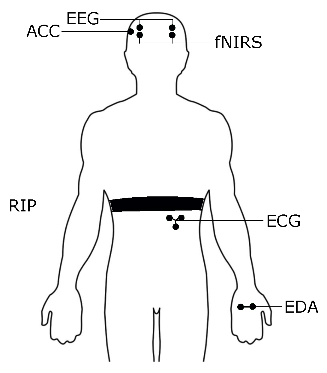
The physiological data were collected using biosignalsplux acquisition devices from PLUX Wireless Biosignals [36] at 1000 Hz and 16-bit resolution. EEG and fNIRS sensors were employed using two channels each (reducing the number of channels to create a close to natural learning environment), positioned around the F7 and F8 positions of the 10–20 system [37]. Electronic devices and noise sources, such as WiFi or Bluetooth devices, were not near the sensors in order to avoid noise. The ECG sensor was applied to measure the lead I of the Einthoven system. The EDA sensor was placed in the palm of the non-dominant hand, reducing movement constraints during computer interaction. The RIP sensor was placed in the upper abdominal region to measure the thoracic expansion/compression and the ACC was placed on the right side of the head to measure head movements and overall posture changes. 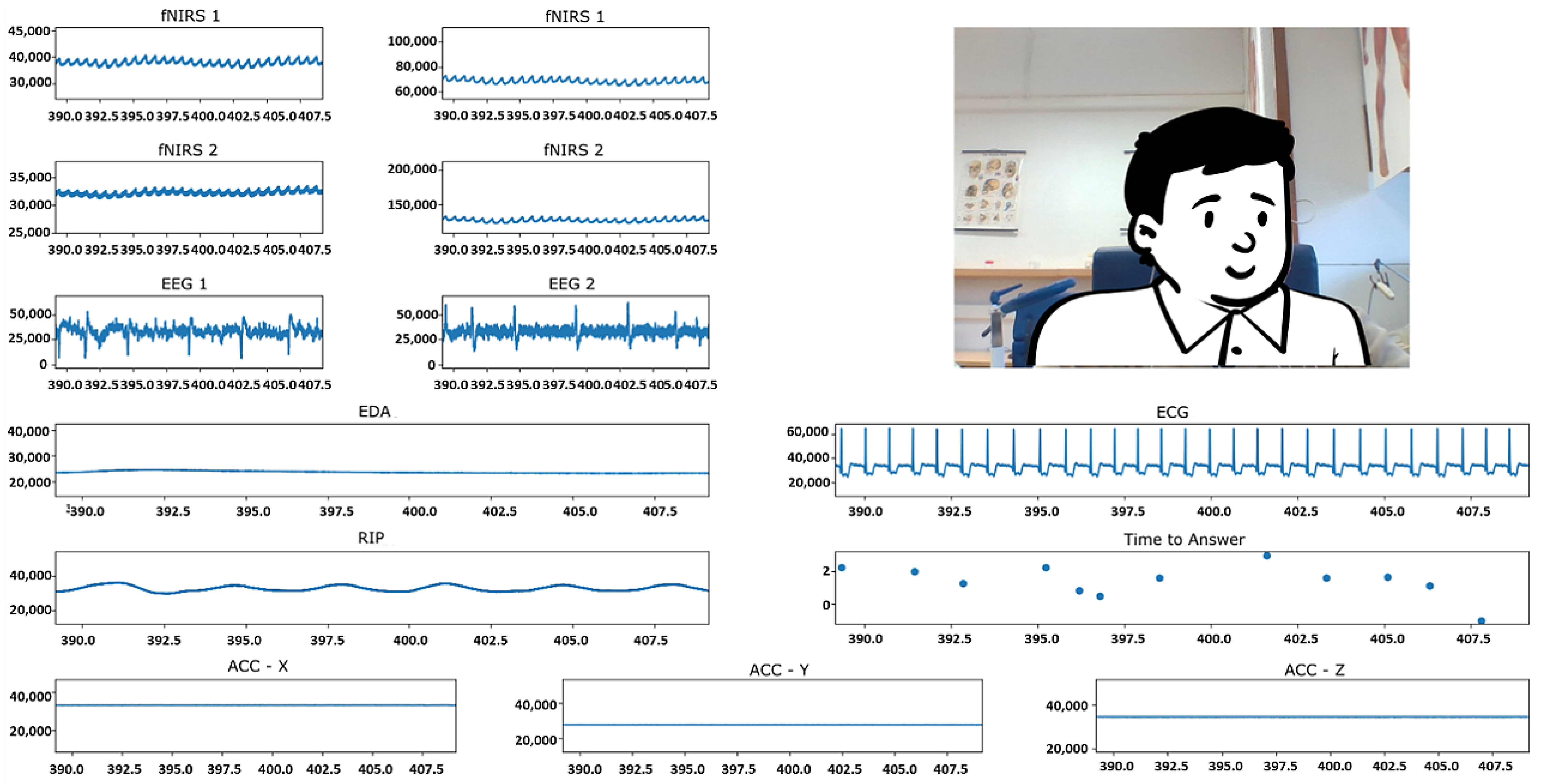The diagram in Figure 1 illustrates the positioning of all sensors. Biosignals data were recorded using OpenSignals, an application provided by PLUX Wireless Biosignals, and stored in TXT format. An example of the acquired biosignals is shown in Figure 2, where all raw signals are shown in arbitrary units.

3.2. Participants

A sample of 8 volunteering subjects (4 females) aged between 20 and 27 years old (M = 22.9, SD = 2.1) participated in this study. Participants were students and recruited at NOVA School of Science and Technology. All participants were Portuguese but fluent in English, and right-handed [38], and none reported suffering from psychological or neurological disorders or taking medication other than contraceptive pills. Written informed consent was obtained before participation according to the approved protocol by the Ethics Committee of the NOVA University of Lisbon. This procedure was performed in an isolated room where all the equipment was disinfected before and after each acquisition due to the current pandemic situation, following guidelines set by the government health entity of Portugal, Direção-Geral de Saúde.

3.3. Tasks

This procedure includes three different tasks: n-back task, mental subtraction task, and Python exercises in a Jupyter notebook [39].

N-back (described in [40]) and mental subtraction were employed as standard cognitive tasks. Rest periods of 60 s were implemented before, between, and after the two main tasks, and 20 s between tasks’ explanations and procedure to avoid contamination from reading the instructions. Finally, a rest period of 10 s between difficulty levels of n-back and between subtraction periods was introduced. Regarding the number of trials, the n-back task consisted of 4 levels with 60 trials each, and mental subtraction had 20 subtraction periods of 12 s, in which, participants had to continuously subtract a given number from the result of the previous subtraction while a visual cue was shown.

Participants took, on average, around 8 min and 30 s ($509\pm 75$ s) to complete the n-back task and 9 min and 7 s ($547\pm 2$ s) to complete the mental subtraction task.

The Python exercises, presented in a tutorial, aim to simulate a close-to-real working task that involves the execution of theoretical and practical examples. This part of the procedure will be analyzed for future purposes and will not be explored in this study.

3.4. Procedure

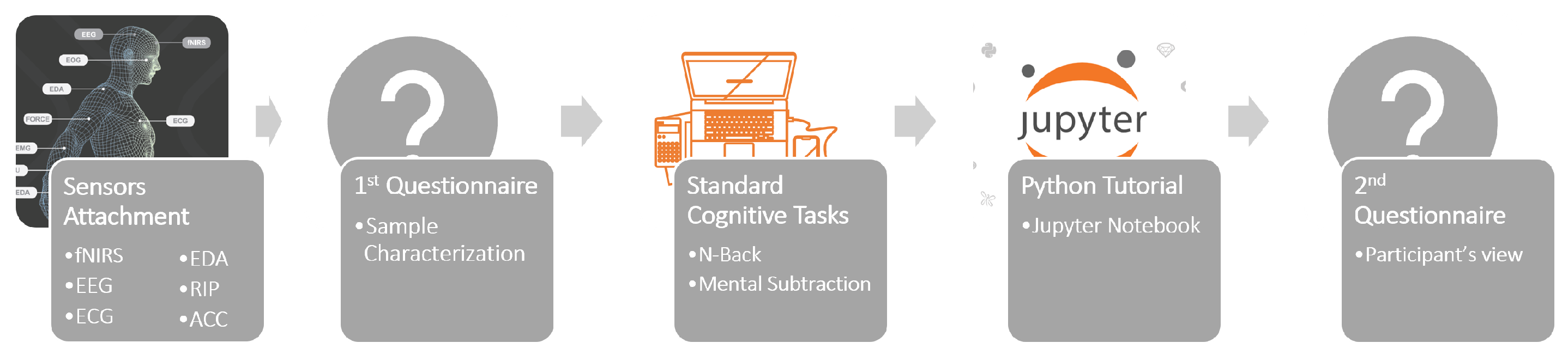
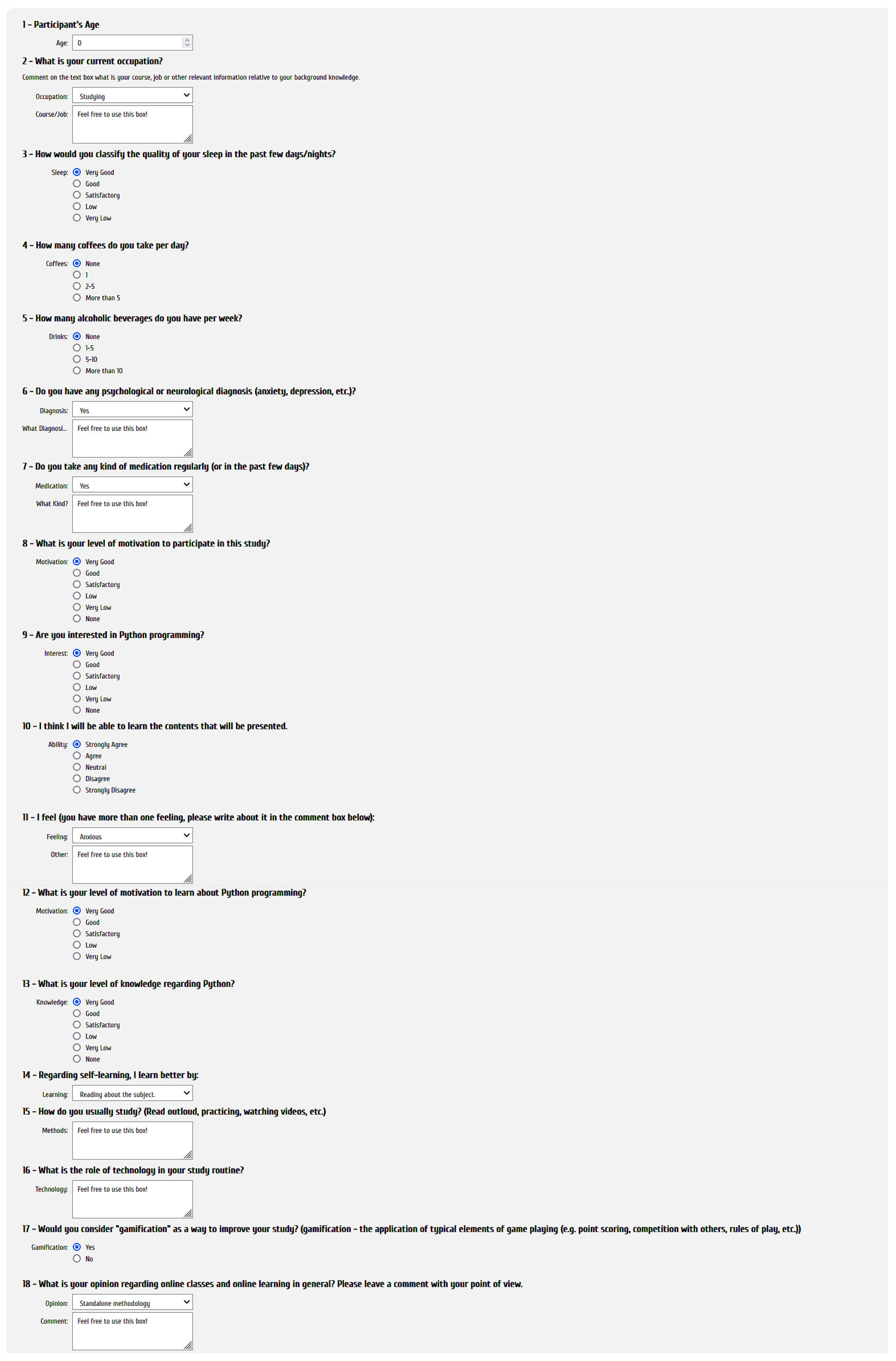
After being in the room, participants were informed about the whole procedure in this experience, all provided written informed consent, and none objected to wearing the sensors. After this, the sensors were attached, and the software with which the participants would interact with was launched. Regarding the experimental procedure, the participants were asked to fill a sample characterization survey with some of their personal information, depicted in the annexed Figure A1. The cognitive tasks that followed included standard psychological tests, namely the n-back task and the mental subtraction task. After completing these cognitive tasks, participants were asked to solve the Python exercises. Finally, a questionnaire was presented regarding the participants’ opinion of the whole experience (whether the duration of the experimental procedure was appropriate, whether the language was understandable, whether the difficulty of the questions was adjusted, etc.). The whole procedure is described visually in Figure 3.

3.5. Signal Processing

Biosignals can be prone to motion artifacts or other noise sources and should be pre-processed for impact minimization. Thus, a second-order band-pass Butterworth finite impulse filter was applied to each acquired biosignal with cut-off frequencies adapted to each of them. A summary of those frequencies is presented in

Table 1. Cut-off frequencies in Hz of the second-order band-pass Butterworth finite impulse filters applied for each acquired biosignal.

Biosignal	Low-Pass (Hz)	High-Pass (Hz)
fNIRS	0.05	1
EEG	1	30
ECG	5	15
EDA	0.016	35
RIP	0.01	1
ACC	0.01	10

.

In the case of the fNIRS sensor, after applying the filter, the modified Beer–Lambert law was applied to convert optical density into relative concentrations of the chromophores of hemoglobin, i.e., oxygenated hemoglobin and deoxygenated hemoglobin using the mes2hb GitHub repository [41].

After pre-processing, the signals were segmented according to the tasks and resting periods. A windowing approach with no overlap was applied to re-segment the segments in 10 s segments. Possible uneven sampling segments were removed according to the following filter: more than 20% of data points with 5 times higher period than the 1 × 10${}^{-3}$ s sampling period or one of the data points has a time difference higher than 0.2 s compared to the adjacent neighbors. Finally, the final half of the segments of each task (n-back and mental subtraction) was removed to make sure that fatigue did not influence our results.

A label of task or baseline was attributed for each extracted segment. Namely, if a given segment belonged to one of the cognitive tasks, the label was task, and if it belonged to one of the rest periods, the label was baseline.

3.6. Feature Extraction

Given the 10 s signal segments, relevant information needed to be extracted to enable the classifiers to find possible relations between them and the given classes. That information was extracted in the form of features using the time series feature extraction library (TSFEL) project [42]. The original TSFEL paper describes all implemented features in detail and presents their corresponding mathematical formulation. Though TSFEL provides a list of 60 features, we only kept 22 features for each segment based on the following criteria: (1) exclude features that were specific to sensors we did not employ (e.g., audio and electromyography); (2) exclude the features that had high computational cost according to the values provided in TSFEL GitHub repository; (3) reduce the number of remaining features to approximately half arbitrarily to reduce the computational cost of extracting the features. The final set of features, their domain, and the corresponding description are enumerated in

Table 2. Extracted features, respective domain, and short description.

Domain	Feature	Description
Statistical	Maximum	Maximum value of a segment.
	Minimum	Minimum value of a segment.
	Polarity	Maximum of segment divided by the minimum.
	Mean	Mean value of a segment.
	Variance	Variance value of a segment.
	Standard Deviation	Standard deviation value of a segment.
	Kurtosis	Kurtosis of a segment.
	Skewness	Skewness of a segment.
Temporal	Mean of Differences	Mean of the derivate of the segment.
	Total Energy	Total energy of a segment in the form of the sum of the squares of all values divided by the time of the segment.
	Area Under the Curve	Area under the curve of the segment using the trapezoid rule.
	Absolute Energy	Same as total energy, but without accounting for the time of the segment.
	Peak to Peak Distance	Absolute value of the peak to peak amplitude of a segment.
	Entropy	Shannon entropy of a segment.
	Slope of Linear Regression	Slope of a linear regression of a segment.
	Zero Crossing Count	Number of times the signal crosses the zero value.
Spectral	Fundamental Frequency	Frequency of the first prominent peak of the segment’s frequency spectrum.
	Maximum Frequency	Maximum frequency of the segment’s frequency spectrum.
	Power Bandwidth	Width of the frequency band in which 95% of its power is located.
	Spectral Distance	Sum of the difference between the frequency spectrum of the segment to the linear regression of the cumulative frequency spectrum.
	Median Frequency	Median frequency of the segment’s frequency spectrum.
	Spectral Entropy	Spectral entropy of the segment’s frequency spectrum.

.

Thus, we extracted 22 features from each signal. This means that, for sensors composed of more than one channel, the number of features multiplies by the number of generated signals. Namely, we have 2-channel EEG, so 44 EEG features; 4 signals of fNIRS (2 chromophores for 2 channels), resulting in 88 features; finally, 3-channel ACC, and thus 66 features. When combining sensors, the number of features sums. Hence, when we consider EEG-fNIRS, for example, the total number of features is 132 (44 + 88).

Unlike other works, such as [43], our feature extraction procedure was generic enough to be applicable to all sensor signals simultaneously.

3.7. Model Training

We used a random forest algorithm to perform the model training to classify the attention events. In this case, the train and test sets were selected by stratified k-folds cross-validator. The models were trained with individual biosignals or their combinations. The different combinations of biosignals depend on the general results of each sensor.

When the datasets are imbalanced, which means that the predictive classes do not exist in the same quantity, the models could produce biased results. In our scenario, the two classes were never exactly in the same quantity, and, therefore, to handle this issue, we applied a random undersampling that consists of sampling from the majority class in order to keep only a part of these points. This way, the majority and the minority classes have the same dataset size [44].

Dealing with numerical features in ML, it is a common approach to normalize the variables to discard inter-subject variability. This way, values of the signals are adjusted to a given scale without modifying signal characteristics. We used a technique called standardizing [45] that subtracts the statistical mean from each value and divides the result by the standard deviation. The technique is described in Equation (1)

$$x^{\prime }=\frac{x-\overline{x}}{std\left(x\right)},$$

(1)

where x is the original array of values, $\overline{x}$ is the mean value of x, $std\left(x\right)$ is the standard deviation of x, and $x^{\prime }$ is the standardized vector.

These statistics were calculated from each feature of the training set and were stored to be applied in the testing set. The final set of values has a mean value of zero and a standard deviation of one. To keep the test set unseen during the training phase, the normalization is first performed to the training set of features, recording each mean and standard deviation. The normalization of the testing is based on the recorded mean and standard deviation of the training set.

Random forest (RF) is a supervised learning algorithm. It is an ensemble of decision trees that produces a more accurate and stable prediction, merging multiple decision trees. To overcome the sensitivity of the decision trees, in a random forest, each tree is trained on different sets of data through bagging, which is a method that randomly samples a data set with replacement. The features considered in each node are from a random subset of features to create an uncorrelated forest of trees whose prediction is more accurate than that of any individual tree. The subset of random features should be smaller than the set of features to avoid this problem. Every decision tree consists of decision nodes, leaf nodes, and a root node. The leaf node of each tree is the final output produced by that specific decision tree. For the final decision, the RF classifier aggregates the results of individual trees. The selection of the outcome follows the majority-voting system, leading to the random forest classifier exhibiting good generalization [46,47]. The subset of features used at each node was limited to the logarithm of the number of features. The number of trees was set to 200 due to computational time cost. The criterion used for the decision trees was Gini, the minimum number of samples to split a node was 2, and the minimum number of samples to be a leaf node was set to 1.

Given that test data should not be included in training data, we applied a stratified k-folds cross-validator to split the data into train/test sets. This method divides the sample into groups of samples (folds) of equal sizes. The prediction function uses k-1 folds for training and leaves one fold out for testing. A stratification process is also part of this method in order to guarantee that each fold contains approximately the same percentage of classes in the training set and the test set [48].

3.8. Model Evaluation

To evaluate a model’s performance, the predicted classes of the samples of the test set are compared with the real classes. In a binary classification, which is the case of this study, the evaluation metrics are based on the following terms [49]:

• True Positive (TP): number of samples predicted positive and with a positive real class;
• True Negative (TN): number of samples predicted negative and with a negative real class;
• False Positive (FP): number of samples predicted positive and with a negative real class;
• False Negative (FN): number of samples predicted negative and with a positive real class.

In this study, we evaluated the models based on their accuracy, which corresponds to the ratio between the number of correctly predicted classes and the number of all predicted classes within the test set (Equation (2)) [49].

$$\mathrm{Accuracy}=\frac{\mathrm{TP}+\mathrm{TN}}{\mathrm{TP}+\mathrm{TN}+\mathrm{FP}+\mathrm{FN}}$$

(2)

In this work, to evaluate the models in terms of accuracy, only models with an accuracy score higher than 60% are significant, since we are considering binary and balanced sets. However, these will still be regarded as poor models if lower than 70%. Given that, in the related work presented in Section 2, the accuracy scores are between 70% and 80%, we consider those as good models in this context. Given that there were no studies with higher accuracy values, we consider very good models to be those achieving values of 80–90%. Thus, models that achieve results higher than 90% accuracy should be carefully analyzed, as it may indicate cases of overfitting and may not generalize well in real applications.

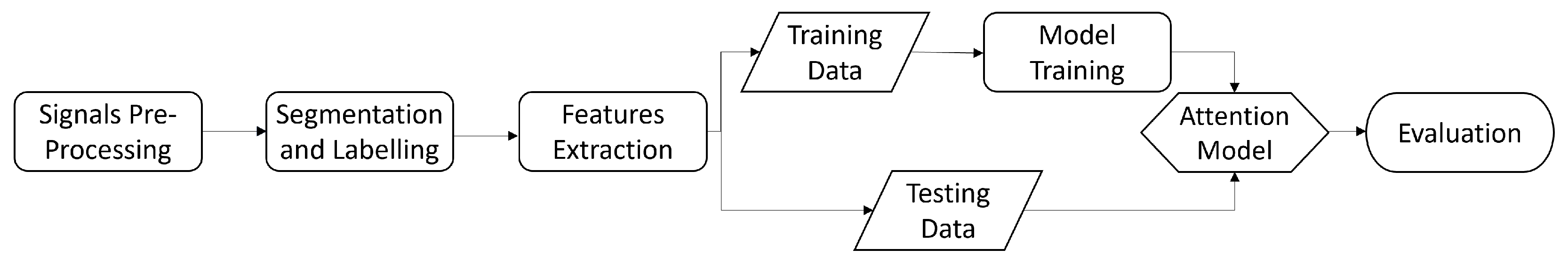
Figure 4 shows a flowchart of the described signal processing steps.

4. Results

Regarding the high number of possible sensor combinations (total of 63) and the required computation time necessary to train models for each combination, we started to train the models with each individual sensor signal and combined best performing ones, and ended by testing the full sensor array. Here, only the results of the best combinations will be presented, and correspond to:

• fNIRS-EEG;
• EEG-ECG;
• EEG-ACC;
• EEG-ECG-ACC;
• fNIRS-EEG-ECG;
• fNIRS-EEG-ECG-EDA.

Regarding the eight participants and the above combination of biosignals, in the end, this work generated 104 different models.

After the biosignals processing part, the application of the filter for uneven sampling to the segments of 10 s removed one single segment from a total of 810.

The segmentation procedure, which differentiates periods of the task and baseline, was performed for each participant, and the total number of each class is presented in

Table 3. Initial number of samples for the considered classes for each participant.

Participant	A	B	C	D	E	F	G	H
# task	54	60	37	56	74	56	52	66
# baseline	48	48	19	47	45	50	50	47

. As already mentioned, in order to use these classes to perform model training, it is important to have a balanced dataset. After randomly downsampling the classes to keep only the original data, the total number of tasks will have exactly the same number as the baseline, given that the task is the majority class for all of the participants and that the number of samples is sufficient to train the classifiers.

Ten folds were selected to apply the stratified k-folds cross-validator given the previously presented size of the final subsets. This way, the minimum test set by fold contains three samples (participant A), and the maximum test set by fold contains ten samples (participant F or G). Therefore, the evaluation of each model is performed in 10 different test folds, and so ten distinct accuracy scores are calculated for each model. The final accuracy is calculated based on the mean of the 10-fold accuracy scores.

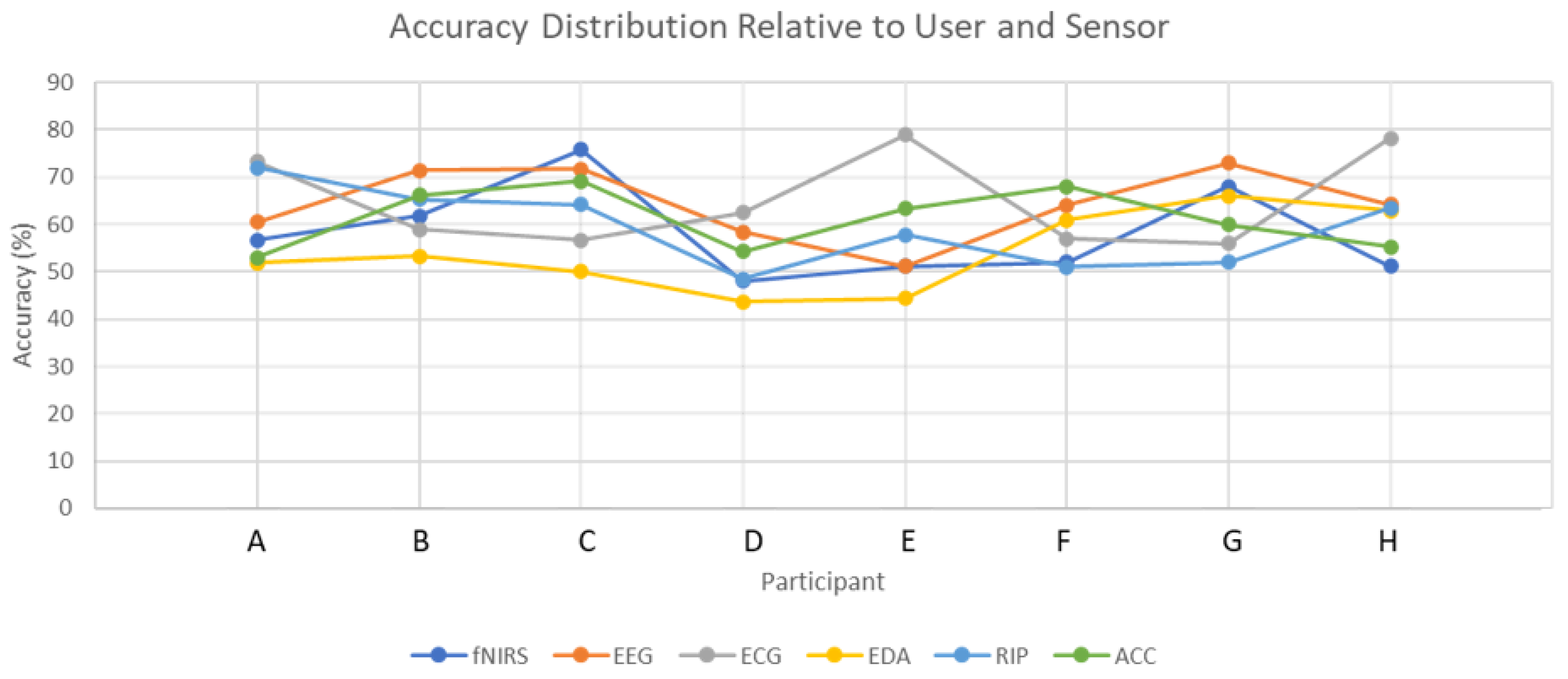
Considering all of the individual models built from the different combinations of sensors,

Table 4. Individual accuracy to predict attention based on each sensor (values in percentage).

Participant	fNIRS	EEG	ECG	EDA	RIP	ACC
A	56.67	60.56	73.22	51.89	72.00	53.00
B	61.78	71.44	59.00	53.33	65.33	66.22
C	75.83	71.67	56.67	50.00	64.17	69.17
D	48.11	58.44	62.44	43.67	48.44	54.33
E	51.11	51.11	78.89	44.44	57.78	63.33
F	52.00	64.00	57.00	61.00	51.00	68.00
G	68.00	73.00	56.00	66.00	52.00	60.00
H	51.22	64.22	78.22	63.00	63.44	55.33

presents the accuracy scores of the models based on each sensor separately to evaluate the performance of each biosignal to predict attention. A graphical representation is shown in the annexed Figure 5.

Except for one participant (A), all of the others achieve better results with training based on more than one biosignal.

Table 5. Individual accuracy to predict attention based on combined biosignals. The accuracy scores with a maximum of two sensors are marked with * and in are in gray.

Participant	Sensors	Accuracy (%)	ROC-AUC (%)
A	ECG	73.22	76.70
B	fNIRS-EEG	72.67	76.80
C	fNIRS-EEG-ECG	80.83	85.00
C *	EEG-ACC	77.50	85.00
D	fNIRS-EEG-ECG-ACC	64.89	66.80
D *	ECG	62.44	64.15
E	EEG-ECG	80.00	79.00
F	EEG-ACC	71.00	74.40
G	fNIRS-EEG	77.00	82.20
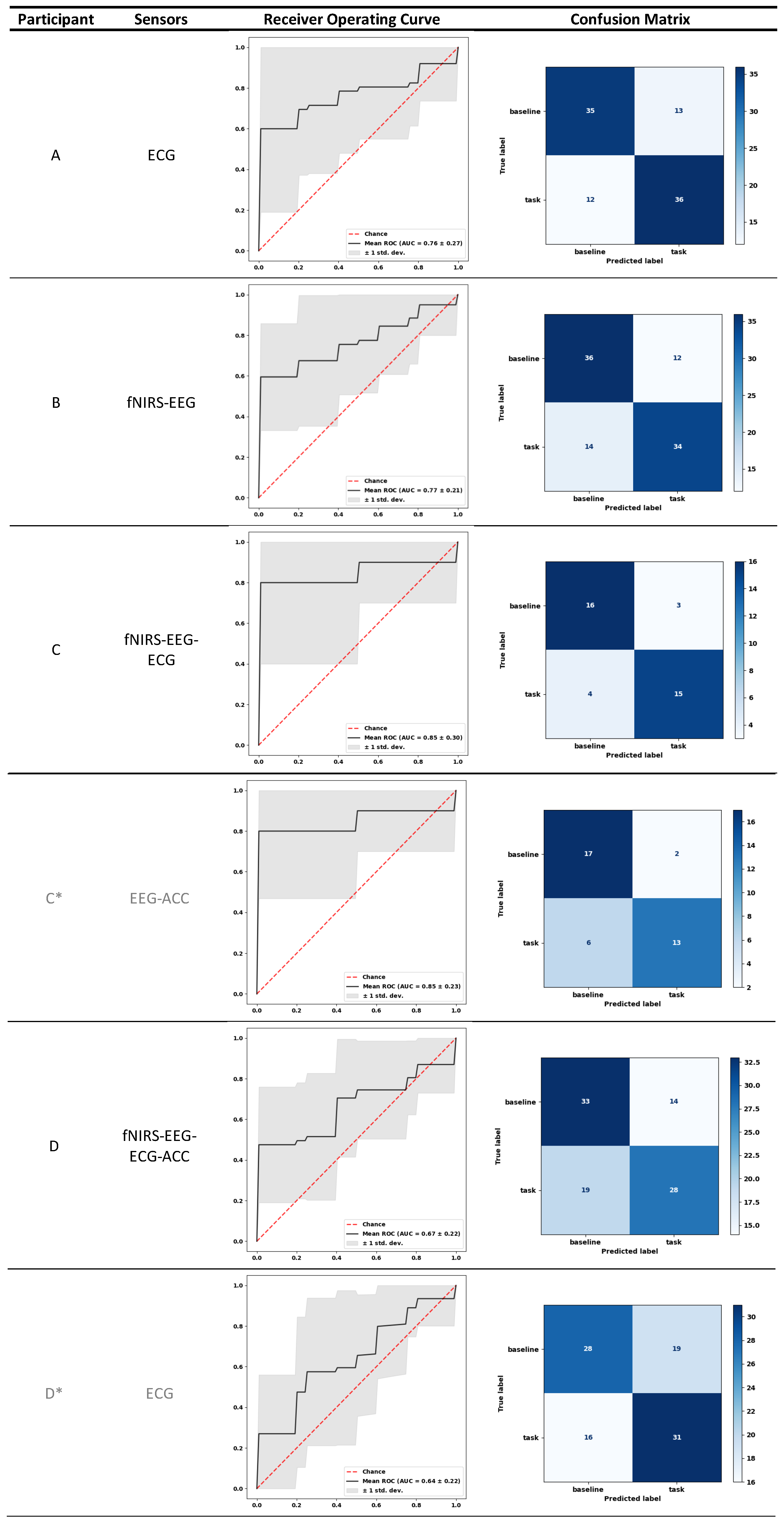
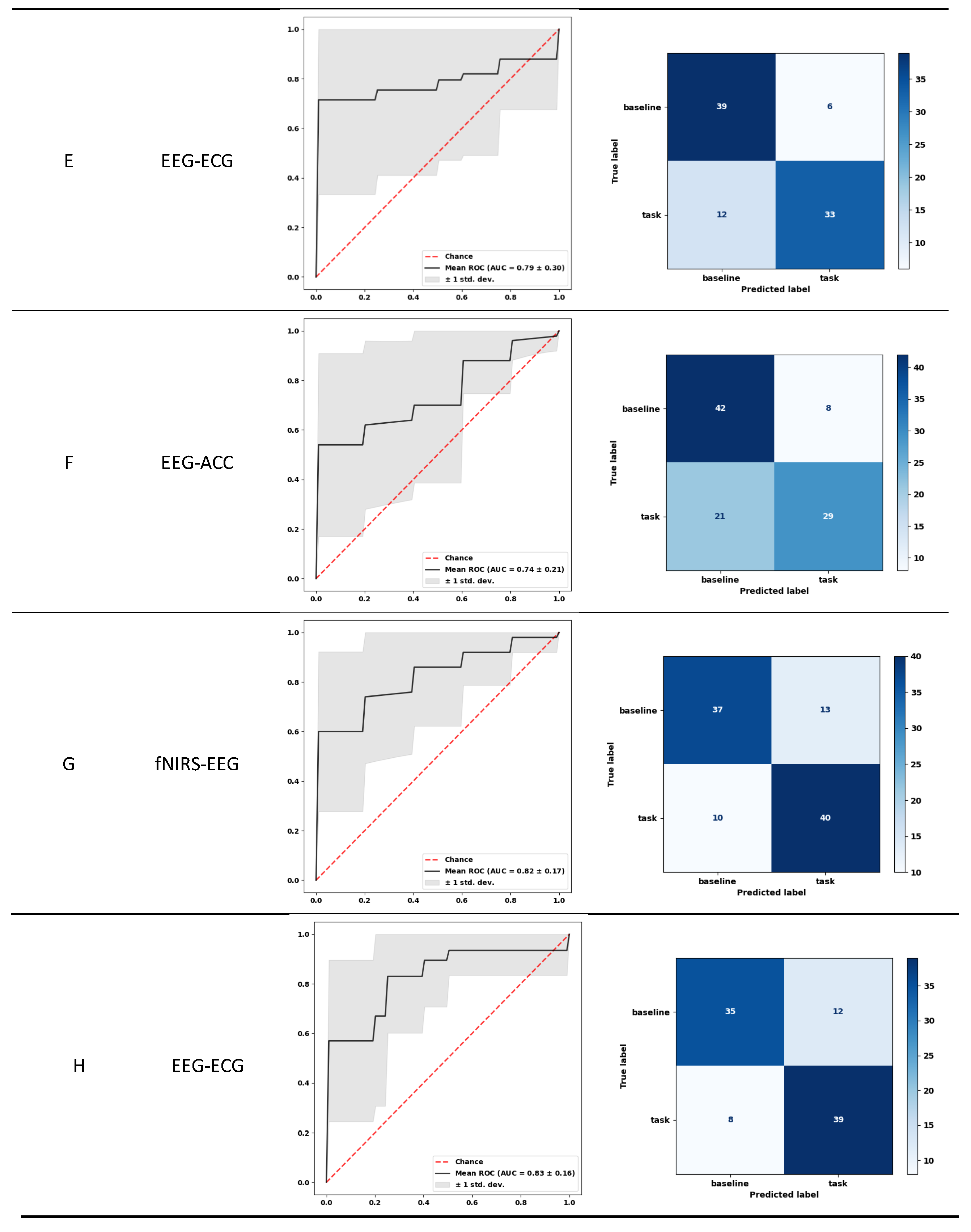
H	EEG-ECG	78.44	82.90

presents the best accuracy scores reached for each participant and the respective area under the curve of the receiver operating curve (ROC-AUC). The respective confusion matrix and ROC curves are shown in Figure A2. To reduce the required equipment, the accuracy of the models trained with a maximum of two sensors is also presented in Table 5.

5. Discussion

This study aimed to assess the feasibility of detecting the participant’s attention state using a multitude of sensors during well-known cognitive tasks. For that, n-back and mental subtraction were selected as candidate tasks to induce attention on individuals. Given the availability and non-intrusiveness of the mentioned sensors, biosignals data were acquired during those tasks. The biosignals were processed, and features with a low computational complexity were extracted and given as an input to classifiers that automatically distinguished between the task and baseline.

After the segmentation and processing phase, we obtained the samples of each subject, as presented in Table 3. We can see that the number of samples for all subjects is close, except for the case of participant C. That was caused by an unexpected disconnection of the device during the acquisition procedure, and so there are no data relative to the mental subtraction task. Aside from the lower combination of sensors, we see from Table 5 that the classification of participant C is better than the performance of all other participants. This happens because the dataset with both tasks is more generic, and thus the cognitive response to the two cognitive tasks may be very distinct. Even though the results may be lower when having both tasks, because of the variability of the responses to those tasks that are not present if we consider a single task (in this case, n-back), the classifiers will be able to generalize better.

Given the number of sensors, it would be important to identify the most suitable ones to detect attention. This will allow us to reduce the acquisition procedure complexity and time in future studies and to interfere as little as possible with the individuals that are performing the cognitive tasks. Thus, a classifier was built for each individual and each sensor. The impact of changing these aspects is presented in Table 4. For example, comparing different sensors for subject E reveals that the range of accuracy values is 44.44–78.89%, the EDA sensor being the least useful (lower accuracy) and the most useful (higher accuracy) being the ECG sensor. On the other dimension, we see that individual differences impact the results, even when using the same sensor. For example, fNIRS values range from 48.11–75.83%, leading us to believe that an individual approach should be considered to obtain the best results possible for each individual. This approach would always require controlled tasks to reveal which are the best sensors for each individual. On the other hand, the combination of various sensors was studied to optimize the achieved results. Once again, different subjects revealed different accuracy levels and a different optimal combination of sensors, pointing toward the direction of an individual-directed tool. The addition of more participants would improve the statistical significance of our results; however, since our approach is based on the individual level, the results presented and discussed would not be altered.

Regarding the most informative biosignals, EEG and ECG have the best mean accuracy scores, i.e., 64.30% and 65.18%, respectively, whereas EDA reaches the worst average performance of 54.17%. Thus, if one would want to apply the same sensors regardless of individual differences with a low number of sensors, a good combination could be the low-channel EEG and ECG. In fact, Table 5 shows that the best combinations for each subject always present either EEG or ECG signals. Surprisingly, fNIRS revealed a poor performance for most subjects. This can be related to a wrong choice for the positioning of the sensor, to a too simplistic processing of the signals, or even to an inadequate emitter–detector distance of the used sensor. Considering the results of EEG being higher than those of fNIRS, this may be related to the poor spatial resolution of the EEG sensor, which can be beneficial in this case, since it may be able to detect activations from greater distances to the sensors than the fNIRS. EDA and RIP sensors did not contribute to good results when considering a low number of sensors and, thus, could be removed in future studies. An interesting aspect is that the EEG sensor with a low number of channels was able to achieve accurate results, especially in combination with other sensors, which proves that ecological validity and the ease of use can be allied with good results.

To the best of our knowledge, previous studies did not consider the individual differences and developed general models. However, our results demonstrate the importance of this consideration. Comparing the methodology of our study with previous studies, many authors solely use cameras [24,25], or cameras associated with motion sensors [23], and achieve results similar to ours, but image acquisition is more invasive than sensors data acquisition. To assess attention, the authors that employed biosignals used only EEG, which was enough to find some relationships with attention [20,22] and achieved good results in predicting attention [21]. However, most of them used 32-channel EEG, which has less ecological validity due to the complex setup than our two-channel sensor. We could not find studies that combined multiple biosignals as we did in this work. Our outcomes demonstrate that the combination of sensors is better in modulating attention than the individual sensors. An interesting finding is the good performance of ECG, which was never explored in previous works and was revealed to be meaningful for attention detection.

6. Conclusions

The work presented in this paper aimed to classify attention events using a random forest algorithm based on features extracted from a wide range of biosignals during the execution of cognitive tasks.

Taking into account the individual differences that are expressed in biosignals and HCI, the model training is performed for each participant separately. These individual differences are confirmed by the accuracy scores obtained for each biosignal separately, which were different from subject to subject. We expected that fNIRS and EEG would have the best results, but fNIRS did not achieve good accuracy scores. EDA and RIP sensors did not contribute to good results, as anticipated.

With the combination of up to three sensors, the achieved accuracy scores were higher than 70%, except for one subject. Therefore, we conclude that, with the acquisition of a combination of only four biosignals (fNIRS, EEG, ECG, and ACC), it is possible to identify attention based on biosignals in cognitive tasks.

As a next step, the HCI variables acquired in the Python exercises task should be explored. Lazar et al. (2017) concluded that HCI tools may be used to assess focused attention and human performance by providing variables such as the time and success in task completion, among others [50]. Variables contributing to cognitive strain and closely related to attention include those that directly disrupt the primary task the worker is attending to, such as interruptions from colleagues [3], notifications [51], or environmental constraints [52]. On the other hand, variables that can promote a balanced working life and attention management, such as quiet working hours [53] and break times [54], can also be tracked through HCI. With all of the variables collected in the last procedure of this study and using the built models as a ground truth of attention, a set of strong correlations between the interaction with the computer and attention could be found.

An alternative that should be considered in future approaches is to find work-related tasks with a high interaction with the computer. With this strategy, the pre-task with acquisition of biosignals could be discarded and the HCI variables could be directly correlated with attention events.

As this study is part of an attention tool proposed by Gamboa et al. (2021), further future work is described in more detail in [9].