J48SS: A Novel Decision Tree Approach for the Handling of Sequential and Time Series Data †


1
Department of Mathematics, Computer Science and Physics, University of Udine, Via delle Scienze, 206, 33100 Udine, Italy
2
R&D Deparment, Gap S.r.l.u., Via Tricesimo, 246, 33100 Udine, Italy
3
Department of Mathematics and Computer Science, University of Ferrara, Via Giuseppe Saragat, 1, 44122 Ferrara, Italy
*
Author to whom correspondence should be addressed.
†
This paper is an extended version of our paper J48S: A Sequence Classification Approach to Text Analysis Based on Decision Trees, published in the 24th International Conference on Information and Software Technologies (ICIST), Vilnius, Lithuania, 4–6 October 2018.
Computers 2019, 8(1), 21; https://0-doi-org.brum.beds.ac.uk/10.3390/computers8010021
Submission received: 11 February 2019
/
Revised: 25 February 2019
/
Accepted: 27 February 2019
/
Published: 5 March 2019
(This article belongs to the Special Issue Selected Papers from the 24th International Conference on Information and Software Technologies (ICIST 2018))
Abstract
:Temporal information plays a very important role in many analysis tasks, and can be encoded in at least two different ways. It can be modeled by discrete sequences of events as, for example, in the business intelligence domain, with the aim of tracking the evolution of customer behaviors over time. Alternatively, it can be represented by time series, as in the stock market to characterize price histories. In some analysis tasks, temporal information is complemented by other kinds of data, which may be represented by static attributes, e.g., categorical or numerical ones. This paper presents J48SS, a novel decision tree inducer capable of natively mixing static (i.e., numerical and categorical), sequential, and time series data for classification purposes. The novel algorithm is based on the popular C4.5 decision tree learner, and it relies on the concepts of frequent pattern extraction and time series shapelet generation. The algorithm is evaluated on a text classification task in a real business setting, as well as on a selection of public UCR time series datasets. Results show that it is capable of providing competitive classification performances, while generating highly interpretable models and effectively reducing the data preparation effort.
1. Introduction
This paper presents J48SS, a novel decision tree learner based on WEKA’s J48 (a Java implementation of C4.5 [1]) (preliminary conference versions of some of its contributions can be found in [2,3]). The algorithm is capable of naturally exploiting categorical, numerical, sequential, and time series data during the same execution cycle. The resulting decision tree models are intuitively interpretable, meaning that a domain expert may easily read and validate them.
Temporal data is of most importance in the extraction of information in many applications, and it comes in at least two flavors: it can be represented either by a discrete sequence of finite-domain values, e.g., a sequence of purchases, as well as by a real-valued time series (for instance, think of a stock price history). Sometimes, temporal information is complemented by other, “static” kinds of data, which can be numerical or categorical. As an example, this is the case with the medical history of a patient, which may include:
- categorical attributes, with information about the gender or the smoking habits;
- numerical attributes, with information about age and weight;
- time series data, tracking the blood pressure over several days, and
- discrete sequences, describing which symptoms the patient has experienced and which medications have been administered.
Such an heterogeneous set of information pieces may be useful, among others, for classification purposes, such as trying to determine the disease affecting the patient. Another use case is that of phone call classification in contact centers: a conversation may be characterized by sequential data (for instance, textual data obtained from the call recordings), one or more time series (keeping track of the volume over time), and a set of categorical or numerical attributes (reporting, e.g., information pertaining to the speakers, or the kind of call). Unfortunately, different kinds of data typically require different kinds of preprocessing techniques and classification algorithms to be managed properly, which usually means that the heterogeneity of data and the complexity of the related analysis tasks are directly proportional. Moreover, since multiple algorithms have to be combined to produce a final classification, the final model may lack in interpretability. This is a fundamental problem in all domains in which understanding and validating the tranined models is as important as the accuracy of the classification itself, e.g., production business systems and life critical medical applications.
Specifically, the proposed algorithm has been evaluated through two distinct experimental tasks. We first applied it in the business speech analytics setting. The starting point was the observation that phone transcripts may be viewed as a kind of sequential data, where phrases correspond to sequences that can be managed by our algorithm. The proposed solution has been tested on a set of recorded agent-side outbound call conversation transcripts produced in the context of a country-wide survey campaign run by Gap S.r.l.u., an Italian business process outsourcer specialized in contact center services. The considered task consisted of identifying relevant phrases in such transcripts, by determining the presence or absence of a predefined set of tags, that carry a semantic content. The ability of tagging phone conversations may greatly help the company in its goal of introducing a reliable speech analytics infrastructure with a considerable operational impact on business processes, which may help in the assessment of the training level of human employees or in the assignment a quality score to the calls. The importance of analyzing conversational data in contact centers is remarked by several studies [4], based on the fact that the core part of the business still focuses on the management of oral interactions. Other benefits that speech analytics can deliver in such a domain include the tracking down of problematic calls [5], and, more generally, the development of end-to-end solutions to conversation analysis as witnessed, for example, in [6].
The second experiment focused on time series, which play a major role in many domains. For instance, in economy, they can be used for stock market price analysis [7], in the healthcare domain, they may allow to predict the arrival rate of patients in emergency rooms [8], and in geophysics, they convey important information about the evolution of the temperature in the oceanic waters [9]. Specifically, we evaluated the proposed algorithm against a selection of well-known UCR (University of California Riverside) time series datasets [10], focusing on the task of time series classification: given a training dataset of labeled time series data, the goal is that of devising a model capable of labeling new, previously unseen instances. Several techniques have been used in the past for such a purpose, including support vector machines [11] and neural networks [12]. Nonetheless, in all situations when interpretability has to be taken into account, decision trees are still mostly used (see, for instance, [13]).
In both test cases, experimental results show that J48SS is capable of training highly readable models, that nontheless achieve competitive classification performances with respect to previous interpretable solutions, while requiring low training times. In addition, some exploratory results suggest that J48SS ensembles might perform better than those proposed in previous studies, while also being smaller. While we are conscious that some approaches have recently been presented, capable of achieving a higher accuracy on time series classification than our solution (see, e.g., [14]), these typically come short of two distinctive characteristics of J48SS, i.e., the ability of seamlessly handling heterogenous kinds of attributes, which, again, reduces the data preparation effort, and the intuitive interpretability of the generated models.
The paper is organized as follows. Section 2 gives a short account of the main concepts and methodologies used throughout the paper. Section 3 thoroughly describes the extensions made to J48 in order to handle sequential and time series data. Section 4 details the two experimental tasks. Section 5 presents the results of the experiments. Finally, Section 6 briefly recaps the main achievements of the work, and discusses some aspects regarding the power of the proposed algorithm and the characteristics of the datasets where it should be capable of excelling, finding its natural application.
2. Background
This section briefly introduces the main concepts and methodologies used in the paper. Specifically, Section 2.1 presents the J48/C4.5 learner, on which our decision tree model is based. Section 2.2 introduces the sequential pattern mining task, on which we rely to extract meaningful information from training sequences. Finally, Section 2.3 and Section 2.4 give a brief overview of evolutionary algorithms and time series shapelets, which constitute the basis for our management of time series data, respectively.
2.1. The Decision Tree Learner J48 (C4.5)
J48 is the WEKA (Waikato Environment for Knowledge Analysis) [15] implementation of C4.5 [1], which, to date, is still one of the most used machine learning algorithms when it comes to classification. It owes its popularity mainly to the facts that it provides good classification performances, is computationally efficient and it guarantees a high interpretability of the generated models. In short, C4.5 builds a decision tree from a set of training instances following the classical recursive Top Down Induction of Decision Trees (TDIDT) strategy: it starts from the root, and at each node it determines the data attribute (categorical or numerical) that most effectively splits the set of samples into subsets, with respect to the class labels. Such a choice is made according to the Information Gain (IG) and Gain Ratio criteria, both based on the concept of Shannon Entropy. The splitting process continues until a stopping condition is met, for instance a predefined minimum number of instances. In these cases, the corresponding node becomes a leaf of the tree. Once the tree has been built, (post) pruning techniques are typically applied with the aim of reducing the size of the generated model and, as a result, of improving its generalization capabilities (for details on this latter phase, see, for instance, [16]).
2.2. Sequential Pattern Mining
Sequential pattern mining is the task aimed at discovering “interesting” patterns in sequences [17], i.e., patterns that may be useful for supervised or unsupervised learning purposes. Specifically, this work focuses on the problem of extracting frequent patterns, that intuitively are concatenations of symbols that repeatedly appear in a set of sequences, whose frequency is higher than an user-defined minimum support threshold [18]. Many different sequential pattern mining algorithms have been presented over the years, most notably PrefixSpan [19], SPADE [20], and SPAM [21], which share the common drawback of generating, typically, a very large amount of patterns. This is problematic, since:
- it makes it difficult for a user to read and understand the output, and to rely on the patterns for subsequent data analysis tasks, and
- an overly large result set may require a too high resource consumption and too long computation time to be produced.
In order to present a small set of patterns to the user, also reducing the computational burden of the mining tasks, several succinct representations of frequent sequential patterns have been devised. For instance, a frequent closed sequential pattern is a frequent sequential pattern such that it is not included in any other sequential pattern having exactly the same frequency, that is, it is somehow “maximal”. Algorithms capable of extracting closed patterns include CloSpan [22], BIDE [23], ClaSP [24], and CM-ClaSP [25]. An additional feasible alternative is that of sequential generator patterns: contrarily to closed patterns, they are “minimal”, in the sense that a pattern is considered to be a generator if there exists no other pattern which is contained in it and has the same frequency. Observe that, based on the Minimum Description Lenght (MDL) principle [26], generators patterns are to be preferred over closed ones for model selection and classification, being less prone to overfitting effects [27]. In the present work, we rely on the algorithm VGEN [28], which, to the extent of our knowledge, represents the state-of-the-art in the extraction of general, sequential generator patterns. Considering the pattern generalization, VGEN operates in a top-down fashion, starting from the most general patterns down to more specific ones.
A pattern is a sequence of itemsets, which can be in turn be considered as unordered sets of distinct items. An item is an element that may be present in a sequence belonging to the reference dataset. Intuitively, items belonging to the same itemset are meant to occur at the same time. The algorithm begins its execution by generating all single-itemset, single-item frequent patterns. They are then grown by means of the so-called s-extension (that enqueue a new itemset to the pattern) and i-extension operations (that add a new item to the last itemset). Of course, as a pattern undergoes extension operations, its support (i.e., the number of instances in the dataset containing the pattern) tends to decrease, and the growing phase continues until a user-defined minimum support threshold is reached. The algorithm can also generate patterns which are not strictly contiguous, by specifying a maximum gap tolerance between the itemsets.
2.3. Evolutionary Algorithms
Evolutionary Algorithms (EAs) are adaptive, meta-heuristic optimization algorithms, inspired by the process of natural selection, and the fields of biology and genetics [29]. Unlike traditional random search, they can effectively make use of historical information to guide the search into the most promising regions of the search space and, in order to do that, they mimic the processes that in natural systems lead to adaptive evolution. In nature, a population of individuals tends to evolve in order to adapt to the environment; in evolutionary algorithms, each individual represents a possible solution to the optimization problem, and its degree of “adaptation” to the problem is evaluated through a suitable fitness function, which may be single or multi-objective. As the optimization algorithm iterates, the elements of the population go through a series of generations. At each generation, the individuals which are considered best by the fitness function are given a higher probability of being selected for reproduction. As a result, over time, the population tends to evolve toward better solutions. Optimization algorithms may be single- or multi-objective. In particular, multi-objective evolutionary algorithms are capable of solving a set of minimization or maximization problems for a tuple of n functions , where is a vector of parameters belonging to a given domain. A set of solutions for a multi-objective problem is said to be Pareto optimal (or non-dominated) if and only if for each :
- there exists no such that improves for some i, with , and
- for all j, with and , does not improve .
The set of non-dominated solutions from is called Pareto front. Multi-objective approaches are particularly suitable for multi-objective optimization, meaning that they are capable of finding a set of optimal solutions in the final population in a single run. Once such a set is available, the most satisfactory one can be selected by applying a user-defined preference criterion.
The algorithm NSGA-II [30], on which our shapelet extraction strategy is based, relies on a Pareto-based multi-objective binary tournament selection strategy with a rank crowding better function: all elements in the population are sorted into fronts, according to a non-domination criterion. A first front is composed of the individuals which are non-dominated overall. A second one is made by those which are dominated by the elements in the first front only, and so on for the subsequent fronts. Then, pairs of individuals are randomly selected from the population. Finally, a Binary Tournament selection is carried out for each pair, by exploiting a better-function based on the concepts of rank (that considers the front the instance belongs to) and crowding distance (which intuitively measures the proximity between an individual and its neighbors). The operators crossover and mutation are then applied to the selected individuals, with the goal of generating new offspring, i.e., a new generation of solutions. The iterations stop when a predefined criteria is satisfied, such as a bound on the number of iterations, or a minimum fitness increment that must be achieved between subsequent generations. An overview of the algorithm NSGA-II applied to the shapelet extraction problem is presented in Figure 1. For more details regarding the specific implementation, see Section 3.2.
Generalization can be defined as the ability of a model to achieve a good performance on new, previously unseen instances, not belonging to the original training set. Conversely, overfitting is a phenomenon that arises when a model too closely fits a specific and limited set of examples, thus failing in applying its knowledge to new data. Given their design, evolutionary algorithms naturally tend to generate solutions that are as good as possible with respect to a given set of instances, against which the fitness function is evaluated, without considering the performances on possible new cases. This may be a problem when they are used within a broader machine learning process. For this reason, generalization in evolutionary computation has been recognized as an important open problem in recent years [31], and several efforts are being made to solve such an issue [32]. For instance, ref [31] proposes the usage, through the generations, of a small and frequently changing random subset of the training data, against which to evaluate the fitness function. Another solution is given by bootstrapping, that is, repeatedly re-sampling training data with replacement, with the goal of simulating the effect of unseen data. The errors of each solution with respect to the bootstrapped datasets are then evaluated, speculating that the most general solutions should exhibit a low variance among the different samples [33]. Also, an early stopping-like strategy may be used for the evolutionary process, based on an independent validation set [34]. Finally, other approaches are based on the idea of reducing the functional complexity of the solutions, which is not to be confused with the concept of bloat (that is, an increase in mean program size without a corresponding improvement in fitness). In fact, as shown in [35], bloat and overfitting are not necessarily correlated.
2.4. Time Series Shapelets
As extensively reported in the literature, time series classification is a difficult problem. A commonly adopted solution is based on a preliminary data discretization step relying on strategies like Equal Width or Equal Frequency binning, or more elaborate approaches such as Symbolic Aggregate Approximation [36]. As a result, a discrete, symbolic representation of the time series is obtained, which may be handled by traditional pattern mining algorithms [17]. Due to its simplicity, many studies have pursued such an approach, for instance [37,38]; still, its downsides typically include information loss, and a reduced interpretability of the final results. Other strategies make use of patterns that may be extracted straight from the numerical data, such as time series shapelets. Shapelets have been first defined in [39] as contiguous, arbitrary-length time series subsequences which are in some sense maximally representative of a class. The idea is that they should be capable of capturing local features of the time series, that ought to exhibit a higher resistance to noise and distortions than global ones. Figure 2 shows an example of a shapelet capturing a local pattern in a time series.
Given their definition, it is possible to calculate the total number of shapelets that can be extracted from a given set of sequences. Let us consider n instances, and define as the length of the ith instance’s time series. Then, the total number of shapelets that may be generated is . Searching such a huge space for the best shapelets in an exhaustive manner is unfeasible and, for this reason, several studies have focused on how to speed up the shapelet extraction process [40,41,42,43,44,45,46], by means, for instance, of heuristics-driven search, or random sampling of the shapelet candidates. Tipically, shapelets are used as follows. Given a training dataset composed of time series, k shapelets are extracted through a suitable method. As a result, every instance is characterized by k predictor attributes, each encoding the distance between the corresponding shapelet and the instance’s time series. As for the specific distance metric, for its speed and simplicity, most studies have relied on Euclidean distance, although Dynamic Time Warping [47] or Mahalanobis distance [48] have been experimented as well: the resulting value is the minimum distance between the time series and the shapelet, established by means of a sliding window approach.
3. Materials and Methods
This section presents J48SS, a new decision tree learner based on J48 (WEKA’s implementation of C4.5, release 8 [15]): Section 3.1 describes the extensions we made to the original algorithm to manage sequential data, while Section 3.2 describes how we handle time series.
3.1. Handling of Sequential Data
To extract meaningful information from sequential data, J48SS relies on the VGEN frequent closed pattern extraction algorithm [28]. The following sections thoroughly describe all the changes that we made in order to seamlessly integrate the two algorithms. For further details regarding the main recursive procedure used in the tree building phase, see the code of Algorithm 1.
3.1.1. Adapting VGEN
One of the key component of the proposed tree learner is a suitable adaptation of the algorithm VGEN. As already pointed out, such an algorithm builds frequent generator patterns in a top-down manner, until a user-defined minimum support threshold is met. Since we are not interested in obtaining a set of frequent patterns, but rather highly discriminative patterns that may be used in the classification task, the information gain criterion has been integrated into the algorithm. In the following, such an integration is described in detail for the (simpler) two-class classification problem; however, it can be easily generalized to multi-class classification, e.g., following a one-vs-all strategy.
To begin with, we observe that the information gain of a pattern can be computed by partitioning the dataset instances in two classes: the class of the instance that satisfy it, and the class of those that do not. It is worth noticing that the information gain of a pattern is directly affected by its support (see [49]: often patterns with a very high or low support are not really useful, as the former are just too common, and the latter have a too limited coverage among the instances in the dataset).
Based on such assumptions, Cheng et al. [49] presents a strategy to derive an upper bound to the information gain, taking into account the support of the pattern. A graphical account of the relationships between such an upper bound and the support is given in Figure 3 (solid curve), which refers to data collected from a randomly-generated binary class dataset. As expected, looking at the picture from left to right, we observe that an increase in the support causes an increase in the upper bound, until it peaks; then, it starts decreasing as the relative support approaches 1. In addition, the picture shows (red dots) the information gain and support of each pattern extracted by VGEN on the same dataset.
Hence, given a calculation method for the upper bound, we can easily define a stopping criterion for the pattern growing process (remember that, as a pattern grows, its support may only decrease). Throughout the pattern generation process, a dedicated variable stores the best information gain found up to a certain moment. Then, given a pattern, the following strategy may be used to decide if it is worth growing or not: if the derivative at the point in the curve associated with the value of the support is positive or equal to zero, then growing it may only decrease the upper bound or leave it unchanged. It follows that if the best information gain obtained so far is already greater than or equal to the information gain upper bound of the pattern, the growing process can be stopped. As a matter of fact, such a strategy works as a second stopping condition, which is combined with the minimum support threshold method.
As we shall see in Section 3.1.2, VGEN is called at each node by the main decision tree learning procedure, in order to obtain a candidate pattern that may be used for the split operation (refer to the code of Algorithm 1). Thus, at that stage, we are interested in obtaining just the single most useful pattern, rather than a set of patterns, as returned by the original VGEN algorithm. Observe, however, that sometimes it is not possible to just select the most informative one, as it might overfit training data. In order to customize the output of the algorithm, we proceed as follows. The best pattern (in terms of information gain) for each encountered pattern size is stored. Then, at the end of the algorithm, the following formula, inspired again by the MDL principle [26], is evaluated for each pattern:
where is a weight that can may customized by the user, is the information gain of the pattern, divided by the highest information gain observed, and is the length of the pattern, divided by that of the longest pattern that has been discovered (in number of items). Then, the pattern that minimizes the value of such a formula is selected, thus, intuitively, the larger the user sets the weight, the longer and more accurate (at least, on the training instances) the extracted pattern will be. Conversely, smaller weight values should lead to a shorter, and more general, pattern being selected. In essence, setting W allows one to control the level of abstraction of the extracted patterns.
3.1.2. Adapting J48 to Handle Sequential Data
As we have already pointed out, the decision tree J48 is able to hand both categorical and numerical features. Our extension J48SS introduces the capability of managing sequences as well, which are represented as properly formatted strings. J48SS somehow resembles the solution outlined in [50], where the authors propose a decision tree construction strategy for sequential data. It improves that one mainly in three respects:
- we rely on a well-established and performing algorithm, such as J48, instead of designing a new one;
- we are able of mixing the usage of sequential and classical (categorical or numerical) data in the same execution cycle;
- our implementation allows the tuning of the abstraction level of the extracted patterns.
The first modification concerns the splitting criterion. Instead of relying on the gain ratio, we consider the so-called normalized gain [51], which is defined as:
where n is the split arity. Note that considering the normalized gain allows for a straightforward integration between the decision tree learner and the modified VGEN algorithm, since such a metric is the same as the information gain for binary splits, as in the case of a pattern-based split (based on the presence or absence of the pattern in the instance).
At each node of the tree, the learning algorithm first determines the most informative attribute among the categorical and numerical ones. Then, it calls VGEN, passing two fundamental parameters:
- the weight W, in order to control the abstraction level of the extracted pattern, and
- the normalized gain of the best attribute found so far, which, as previously described, can be used to prune the pattern search space.
Once VGEN terminates, if a pattern is returned, its normalized gain is compared with the best previously found. If it is found to be better, then a binary split is created on the basis of the presence or absence of the pattern; otherwise, the best numerical or categorical attribute is used.
In Table 1, we list the six parameters that have been added to J48SS, with respect to the original J48, in order to handle sequential data. Observe, in particular, the role of maxGap, that allows one to tolerate gaps between itemsets: in the text classification context, this gives the possibility to extract and apply ngrams capable of tolerating the presence of some noisy or irrelevant words. Observe that, in general, the larger the value of maxGap, the slower the algorithm.
Although having to tune six parameters may seem rather complicate, it should be observed that maxTime is just an upper bound on the running time of the algorithm, and thus it may simply be left at its default value. The parameter useIGPruning should just be left at True as well, since its activation may speed up the computation time of the algorithm. For what concerns maxGap, maxPatternLength, and minSupport, their value should be suggested by domain knowledge. Hence, just one parameter, namely, patternWeight, has to be tuned, for example by cross-validation.
Figure 4 shows a typical J48SS decision tree that makes use of sequential, categorical, and numerical data, built by integrating the proposed extension to WEKA data mining suite [15]. The considered dataset is characterized by three features: sequence_attribute, which is a string representing a sequence of itemsets; attribute_numeric, that has an integer value; attribute_nominal, which may only take one out of a predefined set of values. The class is binary and its labels are: class_0 and class_1. The first test, made at the tree’s root, determines whether a given input sequence contains the pattern or not, checking if there exists an itemset containing A, B, followed (within the maximum allowed gap) by an itemset containing D. If this is the case, the instance is labeled with class_0; otherwise, the tree proceeds by testing on the numerical and categorical attributes.
3.2. Handling of Time Series Data
To extract meaningful information from time series data, J48SS relies on NSGA-II [30]. As in the case of sequential data, this section presents all the changes that have been made in order to integrate the two algorithms together. Specifically, Section 3.2.1 describes the evolutionary algorithm implementation, while Section 3.2.2 illustrates the extensions made to J48.
3.2.1. Using NSGA-II to Extract Time Series Shapelets
Evolutionary algorithms have already been profitably used in different phases of the decision tree learning process [52]. In order to describe how we adapted NSGA-II for the task of shapelet generation, in the following we will discuss:
- how the population (i.e., potential solutions) is represented and how it is initialized;
- how the crossover and mutation operators are defined;
- which fitness function and constraints are used;
- which decision method is followed to select a single solution from the resulting front, given that, as we shall see, we are considering a multi-objective setting.
Differently from the majority of previous works, in our solution we do not require shapelets to be part of any training time series: once they are initialized with values taken from the time series data, they may evolve freely through the generations. As for the implementation of the evolutioary algorithm, we relied on the jMetal framework [53].
Representation of the Solutions and Initial Population. In order to make it easier for us to define the mutation operator, we decided to represent each shapelet in the population by an ordered list of binary arrays, each one of them encoding a floating point value in IEEE 754 double-precision 64 bit format (see Figure 5): the first, leftmost bit establishes the sign of the number, the following 11 bits represent the exponent, and the remaining 52 bits encode the fraction.
As for the initialization of the population, the step is performed on each instance as follows: first, a time series is randomly selected from the dataset; then, a begin and an end index are randomly generated. The shapelet corresponds the portion of the time series that lies between the two indexes.
Crossover Operator. As for the crossover operator, we rely on an approach similar to the single-point strategy [29]. Given two parent solutions, that is, two lists of binary arrays, a random index is generated for each of them. Such indexes represent the beginning of the tails of the two lists, that are then swapped between the parents, generating two offspring. Figure 6 graphically represents the crossover operation, where the two indexes happen to have the same value. Observe that, in general, the two offspring may have a different length with respect to those of the two parents.
Mutation Operator. A properly designed mutation operator should not try to improve a solution on purpose, since this would bias the evolution process of the population. Instead, it should produce random, unbiased changes in the solution components [29]. In the present approach, mutation is implemented by randomly flipping bits in the binary array representation of the elements composing the shapelet. Since we rely on the IEEE notation, the higher the index in the array, the less significant the corresponding bit. Taking that into account, we set the probability of flipping the ith bit to be , where is the overall mutation probability, governed by the mutationP parameter. Intuitively, by employing such a formula, we effectively penalize flipping the most significant bits in the representation, avoiding sharp changes in the values of the shapelets that might interfere with the convergence of the algorithm to a (local) optimum. Finally, when randomly flipping the bits leads to non-valid results (NaN in the IEEE 754 notation), we simply perform a further random flip in the exponent section of the binary array.
Fitness Function. In our implementation, we make use of a bi-objective fitness function. The first one is that of maximizing the information gain (IG) of the given shapelet, as determined on the training instances belonging to the specific tree node: observe that such a measure corresponds to the normalized gain, since a split over a shapelet is always binary. To calculate the IG of a shapelet, first its minimum Euclidean distance with respect to every time series is established, by means of a sliding window approach. Then, the resulting values are dealt with following the same strategy as the one used by C4.5/J48 for splitting on numerical attributes (see, for instance, [1]). Observe that, in principle, one may easily use any other distance metric in the objective.
The second objective is that of reducing the functional complexity [35] of the shapelet, so to fight against undesirable overfitting phenomena that might occur if considering only the first objective. To do so, we make use of the well-known Lempel-Ziv-Welch (LZW) compression algorithm [54]: first, we apply such an algorithm to the (decimal) string representation of the shapelet, and then we evaluate the ratio between the lengths of the compressed and the original strings. Observe that such a ratio is typically less than 1, except for very small shapelets, in which compression might actually lead to longer representations, given the overhead of the LZW algorithm. Finally, NSGA-II has been set to minimize the ratio, following the underlying intuition that “regular” shapelets should be more compressible than complex, overfitted ones. As a side effect, also extremely small (typically singleton) and uninformative shapelets are discouraged by the objective.
Given the fact that we use a bi-objective fitness function, the final result of the evolutionary process is a set of non-dominated solutions.This turns out to be an extremely useful characteristic of our approach, considering that different problems may require different levels of functional complexities of the shapelets in order to be optimally solved. As we shall see, one may easily achieve a a trade-off between the two objectives by simply setting a parameter. It is worth mentioning that we also tested other fitness functions, inspired by the approaches described in Section 2.3. Among them, the best results have been given by:
- an early-stopping strategy inspired by the separate-set evaluation presented in [34]. We first partition the training instances into two equally-sized datasets. Then, we train the evolutionary algorithm on the first subset, with a single-objective fitness function aimed at maximizing the information gain of the solutions. We use the other dataset to determine a second information gain value for each solution. During the execution of the algorithm, we keep track of the best performing individual according to the separated set, and we stop the computation after k non improving evolutionary steps. Finally, we return the best individual according to the separated set;
- a bootstrap strategy inspired by the work of [33]. The evolutionary algorithm evaluates each individual on 100 different datasets, built through a random sampling (with replacement) of the original dataset. Two objectives are considered: the first one is that of maximizing the average information gain of the shapelet, as calculated along the 100 datasets, while the second one tries to minimize its standard deviation, in an attempt to search for shapelets that are good in general.
As a matter of fact, both these strategies exhibited inferior accuracy performance than the previously discussed solution. While for the first approach this might be explained by the fact that it greatly reduces the number of training instances (a problem that is exacerbated in the smallest nodes of the tree), the reason behind the poor performance of the second one is still unclear, and deserves some further attention.
Decision Method. In order to extract a single shapelet out from the resulting front of Pareto-optimal solutions, we evaluate each individual with respect to the following formula:
where is a weight that can be customized by the user (by the patternWeight parameter), is the compression ratio of the shapelet, and is the information gain of the shapelet, both divided by the respective highest values observed in the population. The solution that minimizes the value of such a formula is selected as the final result of the optimization procedure, and is returned to the decision tree for the purpose of the splitting process. Intuitively, large values of W should lead to a highly accurate shapelet being extracted (at least, on the training set). Conversely, a small value of W should result in less complex solutions being selected. Note that the approach is quite similar to the one we used to handle sequential data: in fact, this allows us to seamlessly rely on the same weight W in both cases.
3.2.2. Adapting J48 to Handle Time Series Data
Consider now the execution of J48SS on time series data, concerning the tree growing phase. Algorithm 1 illustrates the main procedure that is used during the tree construction phase: it takes a node as input, and proceeds as follows, starting from the tree root. If the given node already achieves a sufficient degree of purity (meaning that almost all instances are characterized by the same label), or any other stopping criteria is satisfied, then the node is turned to a leaf; otherwise, the algorithm has to determine which attribute to rely on for the split. To do so, first it considers all classical attributes (categorical and numerical), determining their normalized gain value (see Section 3.1.2), according to the default C4.5 strategy. Then, it centers its attention on string attributes that represent sequences: VGEN is called in order to extract the best closed frequent pattern, as described in Section 3.1. Then, for each string attribute representing a time series, it runs NSGA-II with respect to the instances that lay on the node (see the details presented in the remainder of the section), obtaining a shapelet. Such a shapelet is then evaluated as if it was a numerical attribute, considering its Euclidean distance with respect to each instance’s time series (computation is sped up by subsequence distance early abandon strategy [39]), and thus determining its normalized gain value, that is compared to the best found one. Finally, the attribute with the highest normalized gain is used to split the node, and the algorithm is recursively called on each of the generated children.
| Algorithm 1 Node splitting procedure |
|
As for the input parameters of the procedure for the shapelet extraction process, they are listed in Table 2. With the exception of patternWeight, which determines the degree of complexity of the shapelet returned to the decision tree by NSGA-II (see Algorithm 1), they all regulate the evolutionary computation:
- crossoverP determines the probability of combining two individuals of the population;
- mutationP determines the probability of an element to undergo a random mutation;
- popSize determines the population size, i.e., the number of individuals;
- numEvals establishes the number of evaluations that are going to be carried out in the optimization process.
Of course, when choosing the parameters, one should set the the number of evaluations (numEvals) to be higher than the population size (popSize), for otherwise high popSize values, combined with small numEvals values, will in fact turn the evolutionary algorithm behaviour to a blind random search. Each parameter comes with a sensible default value that has been empirically established. However, a dedicated tuning phase of patternWeight and numEvals is advisable to obtain the best performance.
4. Experimental Tasks
This section presents the two analysis tasks on which we evaluate J48SS, namely, tagging of call conversation transcripts (Section 4.1) and time series classification (Section 4.2). All models have been trained on a common, i5 powered, laptop.
4.1. Call Conversation Transcript Tagging Task
In the following, we provide (i) a brief overview of the contact center domain, in which the analysis task takes place; the details regarding the experimental procedures we followed; the data preparation and model training steps.
4.1.1. Domain and Problem Description
Telephone call centers are more and more important in today’s business world. They act as a primary customer-facing channel for firms in many different industries, and employ millions of operators (also referred to as agents) across the globe [55]. Call centers may be categorized according to different parameters. Particularly significant is the distinction between inbound (answering incoming calls) and outbound (making calls) activities. Regardless of its specific characteristics, a large call center generates great amounts of structured and unstructured data. Examples of structured information include the tracking of involved phone numbers, call duration, called service, and so on, while textual notes and call recordings are typical forms of unstructured information.
The activity we are going to consider is the analysis of the behavior of agents in calls done for an outbound survey service offered by Gap. When executing outbound calls, agents are requested to strictly follow a pre-established script: in order to classify a call as a successful one, the script must be respected. Such a rigid structure of conversations makes it easy to establish whether or not an agent has fulfilled all the steps in the relevant script.
In such a context, machine learning techniques can be exploited to learn appropriate models to be used to check the presence or absence of specific tags in call transcripts. For any given domain, it is possible to identify a set of tags that allow one to detect the presence of certain contents in the conversation. Despite its simplicity, such an analysis turns out to be extremely useful for the company.
Typically, the behavior of an agent is manually inspected by supervising staff. The inspection consists in listening to a number of randomly-chosen calls of the agent. Such a work is extremely time-consuming and it requires a significant amount of enterprise resources. The possibility of a fully automatic analysis of conversation transcripts has thus a strong impact: it allows the staff to identify potentially “problematic” calls that require further screening, thus considerably reducing the overall time needed for verification, and increasing the global efficacy of the process. On the basis of the outcomes of the analysis task, the supervising staff can identify those agents who need further training, and also get an indication of the specific deficiencies that must be addressed.
4.1.2. Experimental Setting
In this section, we describe the setup of the experimentation carried out with J48SS, with the aim of enriching call transcripts with relevant tags. For the outbound survey service of choice, we considered the following tags:
- age: the agent asked the interviewed person his/her age;
- call_permission: the agent asked the called person for the permission to conduct the survey;
- duration_info: the agent gave the called person information about the duration of the survey;
- family_unit: the agent asked the called person information about his/her family unit members;
- greeting_initial: the agent introduced himself/herself at the beginning of the phone call;
- greeting_final: the agent pronounced the scripted goodbye phrases;
- person_identity: the agent asked the called person for a confirmation of his/her identity;
- privacy: the agent informed the called person about the privacy implications of the phone call;
- profession: the agent asked the interviewed person information about his/her job;
- question_1: the agent pronounced the first question of the survey;
- question_2: the agent pronounced the second question of the survey;
- question_3: the agent pronounced the third question of the survey.
In Table 3 some examples of transcriptions with the associated tags are presented. Observe that tags are general concepts, that are independent from the specific service under consideration. For example, the greeting_initial tag may apply to different services.
The training and test datasets for the machine learning models have been built starting from a set of 482 distinct outbound calls. Each call has been subdivided into chunks (phrases delimited by silence pauses), and then each chunk has been transcribed by means of an internally-developed solution based on the Kaldi automatic speech recognition toolkit [56]. The result is 4884 strings, that have been manually labeled by domain experts, in a way that each instance is characterized by the transcription, and by a list of Boolean attributes that track the presence or absence of each specific tag. Table 4 reports the number of positive and negative instances for each tag. The resulting dataset has been split into a training (, 3696 instances) and a test (, 1188 instances) set, according to a stratified random sampling by group approach, where each single session is a group on its own, so not to fragment a session between the two sets. Finally, observe that the reported word error rate (WER) for the Kaldi model is 28.77%, which may seem overly high if compared with the WER of 18.70% obtained on the same dataset by relying on Google Speech API. Nevertheless, it is actually low enough to allow for the analysis tasks needed by the company to be performed. A detailed account of these aspects is the subject of a forthcoming work about the whole speech analytics process.
4.1.3. Data Preparation and Training of the Model
The training and test datasets for J48SS have been prepared as follows, starting from the data described in the previous section. First, the text has been normalized: all characters have been converted to lowercase, preserving only the alphabetical one. Then, all Italian stopwords have been removed from the chunks. Subsequently, the remaining words have been stemmed through the algorithm PORTER2. To carry out the preprocessing, we relied on Python’s NLTK library. A training and a test dataset have been created for each tag (for a total of 12 dataset pairs), where each of the instances is characterized by just two attributes: the processed text of the chunk and an attribute identifying the presence or absence of the specific tag (class). As for the training phase, we left almost all parameters at their default values, with the exception of minSupport, which has been set to 0.01 (1%), so as to allow for the extraction of uncommon patterns, and patternWeight, which has been set to 1, based on the domain expert knowledge that the survey service requires very specific phrases to be pronounced by the agents. To provide a baseline for the evaluation of the experimental results, we also made use of logistic regression. Such a choice has been driven by the necessity, expressed by the company, of relying only on interpretable models and led us to neglect, for example, support vector machines, that are often employed for text classification purposes. Three training and test dataset pairs have then been assembled for each keyword, considering different ngram lengths and again a frequency threshold of 1%: unigrams (leading to a total of 177 attributes, plus the class), bigrams (154 attributes, plus the class), and trigrams (102 attributes, plus the class). Given the 12 possible tags, and the 3 different ngram lengths that have been considered, overall 36 training and test dataset pairs have been generated. Logistic models have been trained using WEKA’s logistic algorithm, employing also a feature selection step based on the multivariate, classifier-independent filter CfsSubsetEval [57], that reduced the number of attributes to an average of 12.
4.2. UCR Time Series Classification Task
All the following experiments have been performed on a selection of 16 UCR [10] datasets given the fact that, as witnessed by the literature, it has been broadly used in the machine learning community [14,42,43,45,46]. In addition, such a decision allows us to compare our results to the ones presented in [45]. The details concerning the dataset selection are reported in Table 5. Note that, even if the considered time series all have the same size, J48SS my handle time series having different lengths as well. We pre-processed each of the datasets and, as a result, each instance is characterized by the following set of attributes (other than the class label):
- the original time series, represented by a string;
- the original time series minimum, maximum, average, and variance numerical values;
- the slope time series, derived from the original one and represented by a string;
- the slope time series minimum, maximum, average, and variance numerical values;
The performance of J48SS has then been evaluated with respect to the pre-processed datasets, and against the results presented in [45] (Random Shapelet), that has been chosen for comparison since it is relatively recent approach that also embeds the shapelet generation phase in a decision tree inducing algorithm. Moreover, the paper thorougly describes all aspects of the experimentation phase, which makes our comparison task easier.
As for the experiment workflow, we built 100 J48SS models for each considered dataset. Each tree has been built starting from a different initial random seed, in order to produce statistically sound results. In order to get a better performance, we also tuned, in sequential order, the two parameters that are most likely to control the degree of generalization of the model, i.e., patternWeight and numEvals: the first considering the range ; the second over the values , while leaving all other parameters at their default values. The results of the tuning phase are reported in Table 5. Note that, due to time constraints, we neglected a true grid-search approach that would have allowed us, in principle, to find even better combinations of the two values. We then turned our attention on collecting statistics over several aspects of the algorithm, including its running time, the model sizes, and the generalization capability of the evolutionary approach. In order to do that, we focused on the numEvals parameter, which has been tested over the values .
Again, to ensure statistical soundess, 100 models have been built for each dataset and for each parameter value, varying the evolutionary algorithm initial random seed.
Although, given their interpretability characteristics, we are most interested in the evaluation of single trees, we believe that it is also interesting to get at least some preliminary insights on how ensembles of J48SS models perform. For this purpose, we considered ensembles of 100 trees, built through Weka’s Random Subspace [59] method. Again, we built 100 different models for each dataset, by varying the initial seed and keeping the tuned values for patternWeight and numEvals. We compared the average accuracy results with the ones reported in [43] (Generalized Random Shapelet Forests) which, to the best of our knowledge, has been the only work so far that uses shapelets in a forest inducing algorithm, in the context of time series classification. Along with the accuracy results, we also report the computation times of our approach, even if the Generalized Random Shapelet Forests paper does not exhibit any absolute computation time. Finally, for the sake of clarity, observe that Weka’s Random Subspace function has a seed that should be independently set with respect to the one used by the evolutionary algorithm in order to get proper statistical results; nevertheless, due to time constraints, we did not consider this fact in our analysis. The same reason led us to consider 100-tree ensembles, which is a relatively small number compared, for instance, to the 500 trees that have been suggested as an appropriate ensemble size for traditional random forests [60]. Despite the limits of our preliminary experimentation, we believe that the obtained results are still useful to establish a baseline, and we look forward to carefully investigate the performance of different kinds and sizes of ensembles of J48SS models in future work.
5. Results
In this section, we report the results of the evaluation of J48SS with respect to the tasks of tagging call conversation transcripts (Section 5.1) and classifying time series (Section 5.2).
5.1. Results on Call Conversation Tagging
We evaluated each of the 1188 chunks in the test set against the presence of every possible tag, looking for the concordance between its manual annotations and the ones provided by the corresponding decision tree. In order to evaluate the performance, the following standard metrics have been considered:
- accuracy, which is the fraction of times when a tag has been correctly identified in a chunk as present or absent;
- precision, that is, the fraction of chunks in which a specific tag has been identified as present by the method, and in which the tag is indeed present;
- recall, which shows the proportion of chunks presenting the specific tag, that have been in fact identified as such;
- true negative rate (TNR), that reports the proportion of chunks not presenting the specific tag, that have been classified as negative by the method.
As witnessed by the figures reported in Table 6, our approach can reach a very high accuracy in tagging chunks. However, given the fact that the dataset is unbalanced with respect to the target class, in order to present a more unbiased review of the performances, we also consider the true negative rate, precision and recall indicators. Specifically, the latter is of primary importance to the company, since it may help in revealing which tags are the most difficult to identify. Again, we obtained highly satisfactory results for most of the tags, with the exception of call_permission, that falls slightly under 0.65 precision and recall.
As an example, consider the tag greeting_final. A typical, well-recited closing phrase for the considered service should be of the form: “Ok, we have finished. Thank you for the cooperation and good day, also on behalf of [company_name]. If you allow me, I inform you that [company_name] may recontact you”. Figure 7 presents the model that recognizes the presence of the tag. The tree has just 9 leaves, meaning that, besides the chosen representation, it is very simple and intuitive to read, even for a non computer scientist domain expert. For instance, the tree already discards conversations which do not contain the words recontact and inform and the sequence thank>cooperation. This is plausible, since such elements are very important components of the scripted phrase, that should not be forgotten. Specifically, a rule that may be extracted from the decision tree model is:
IF the current instance contains neither the terms ‘recontact’ and ‘inform’, nor the term ‘thank’ followed by the term ‘cooperation’, THEN label such an instance with class ‘0’.
As for the complexity of the training phase, the considered tree has been built in less than 30 s on a common, i5 powered, laptop, while its application to a new instance is almost instantaneous.
As for the logistic regression approach, surprisingly, the experimental results suggested that the unigram-based models are the most effective in tagging the transcripts. This may be explained in two ways:
- the considered datasets may just not be large enough to justify the use of bigrams and trigrams, or
- tag recognition in calls generated in the context of the considered service may not be a difficult concept to learn, so unigrams are enough for the task.
In Table 7, the detailed results for the unigram models are reported.
By looking at the (macro) average values of the logistic approach, we may notice that most of the performance metrics are very close to the ones provided by J48SS, with the exception of recall (once again, the most important metric in this context), which is lower than the one provided by the decision tree, somehow balanced by a slightly higher precision.
Thus, the result provided by J48SS ares comparable to the ones of the best approach based on logistic regression. Moreover, since such results have been obtained by running J48SS with the default parameters (except for the minimum support value and pattern weight, which have been set following domain expertise), we speculate that an even better performance might be achieved through a dedicated tuning phase. Apart from the mere classification performance, observe also that the use of J48SS entails a much simpler data preparation phase than logistic regression, since the decision tree is capable of directly exploiting textual information. This allows one to avoid the ngram preprocessing step, and the related a-priori choices of the ngram sizes and frequencies altogether. In fact, recall that the ready-to-process datasets for J48SS are very simple, having exactly two attributes, while those for the ngrams-based approach varied from 103 to 178 attributes, a number that required us to perform an additional feature selection step. In addition, sequential patterns should be more resistant to noise in the data than bigrams and trigrams, as they allow to skip irrelevant words thanks to the maxGap parameter. Last but not least, J48SS models are much more understandable to (non computer scientists) domain experts than regression models.
5.2. Results on UCR Datasets Classification
In this section, we present the results of the experiments carried out on the selection of UCR datasets, with respect to single trees (Section 5.2.1) and ensembles of J48SS models (Section 5.2.2).
5.2.1. Results of Single J48SS Models
The results of the experimentation of single J48SS trees are reported in Table 8, together with the accuracies originally presented in [45] (Random Shapelet). Both performances have been obtained by averaging over 100 executions of the algorithms.
The Random Shapelet approach results are obtained by sampling different percentages of the total number of shapelets (ranging from 0.10% to 50%). We may observe that J48SS is capable of achieving an overall better accuracy result than Random Shapelet, despite the fact that we have performed just a mild tuning phase. Thus, we may speculate that an even better performance may be achieved by means of a full-parameter tuning phase, for instance by means of a grid-search approach on a wider search range.
Despite the fact that J48SS has shown an inferior classification performance on some datasets than Random Shapelet, it should be observed that the latter requires very long computation times, especially when the larger sampling values are used [45]: typically hundreds of seconds are needed in order to build a single model on the smaller datasets, and thousands of seconds (or even worse) are required on the larger ones. On the contrary, while J48SS training times tend to increase with the number of evaluations, they are comparatively much lower, as shown in Table 9.
Let us now consider the importance of weight tuning. Figure 8 reports the accuracies (averaged over 100 executions) for datasets ECGFiveD and SonyAIBO, when different values of patternWeight are employed. Observe the very different behaviours shown by the two datasets: while in ECGFiveD the best performance is provided by high-performing shapelets (with respect to the Information Gain), SonyAIBO tends to favor simple patterns. This fact remarks the crucial influence of the parameter patternWeight on the classification performance, and the importance its proper selection.
As for the generalization capabilities of the evolutionary approach, Figure 9 shows the trend of the test set accuracy of the J48SS models, over the number of evaluations, for three selected datasets, leaving all other parameters at their default values. The typically observed behavior is the one of DiatomSize: the accuracy tends to grow as the number of evaluations increases, until it peaks, and then starts to decrease, due to overfitting in the evolutionary algorithm. There are also other two notable tendencies, that have been rarely seen and typical, for instance, of datasets Beef and ECGFiveD: in the former, the accuracy increases consistently, although we may speculate that it would peak, and then decreases if a sufficiently high number of evaluations is given; in the latter, the accuracy decreases steadily, potentially suggesting that the chosen fitness function is failing in avoiding the overfitting.
Let us now discuss the interpretability of the J48SS trees. Figure 10 shows the average and standard deviation of the number of nodes in the trees built on each of the considered datasets. As can be seen, most of the models are quite small, exept for Adiac, ChlorineC, and MedicalIm. We speculate that such an heterogeneity in the model sizes might indicate that different datasets are characterized by different degrees of difficulty, when it comes to the task of deriving a classification strategy. Of course, the user may also adjust the desired size of the decision trees by setting the two parameters of J48SS that control the pre- and post-pruning aggressiveness (already available in J48).
Figure 11 shows one of the J48SS models that have been trained on the Beef dataset. Starting from the root, the tree first checks the distance between the specific shapelet and the time series attribute named TS (the pattern may be easily visualized, for example by plotting its list of values). If such a value is less than 0.109855, then it tests the distance between another shapelet and the time series named TS_slope. If the distance is less than 0.01709, it assigns the class 2 to the instance. It is worth pointing out that not only time series attributes are used by the tree, but also numeric ones, such as the kurtosis value of the original time series and the average value of the slope time series. The specific decision tree has a test set accuracy of 53.33%, a value which is largely superior to the ones provided by the Random Shapelet approach.
Figure 12 shows the shapelet tested at the root of the tree with respect to two time series of the train portion of dataset Beef, the first being representative of class 1, the second of class 5. As it can be seen, the time series having class 1 has a bigger distance than the one having class 5, which is consistent with the splits taken in the decision tree. Finally, we observe that in this case the shapelet is quite short with respect to the time series. However, this is not a common situation in our experiments: other shapelets have emerged whose length is comparable to the one of the considered time series (indeed, the fitness function only indirectly influences the length of the generated shapelets).
5.2.2. Results of Ensembles of J48SS Models
Let us now briefly discuss the results of the experimentation with ensembles of J48SS models. Table 10 reports the average accuracy and training time of the generated models (EJ48SS), with respect to the accuracies reported in [43] (Generalized Random Shapelet Forests, gRSF). Once more, remember that the EJ48SS models are made of just 100 trees, while gRSF employed 500-tree forest. Although the presented results should just be regarded as a baseline for future studies on J48SS ensembles, in 8 out of 16 datasets EJ48SS has been capable of matching or surpassing the performance of the competitor, despite using much smaller models. Moreover, taking into account the observations done in Section 5.2.1, it seems reasonable to assume that better results might be obtained without increasing the size of the ensembles much further, but relying on a thoroughly performed tuning phase instead. We are going to investigate these issues in future studies, also assessing different kinds of ensemble methods.
6. Discussion
The experimental results reported in the previous section allow us to conclude that J48SS is capable of achieving a competitive classification performance with respect to both sequence and time series data classification. Moreover, as a further advantage over previous methods, the trees built by the proposed algorithm are easily interpretable, and powerful enough to effectively mix decision splits based on several kinds of attributes. Finally, as occurred with call conversation tagging, such flexibility allows one to reduce the data preparation effort.
As a matter of fact, the datasets that we used for the experimental tasks did not take full advantage of the capabilities of the new algorithm, as they consist of sequences or time series only, and all static attributes are simply derived ones. In order to fully exploit the potentialities of J48SS, a dataset should contain sequential and/or time series data, and it should include meaningful static (numerical or categorical) attributes, somehow independent from the previous ones. The latter condition means that static attributes should not simply synthesize information already contained in the sequences/time series, but add something per se. Such a dataset has proven to be difficult to find in the literature, maybe because of the lack, until now, of an algorithm capable of training a meaningful model on it. Nonetheless, as mentioned in the introduction, we believe that datasets from the medical domain may have all the desired properties, and we look forward to applying J48SS on such use cases.
7. Conclusions
In this paper, we described J48SS, a novel decision tree inducer based on the C4.5 algorithm. The novel approach is capable of effectively mixing, during the same execution cycle, static (numeric and categorical), as well as sequential and time series data. The resulting models are highly readable, which is a fundamental requirement in those domains in which understanding the classification process is as important as the classification itself, for instance for validation purposes.
The algorithm has been tested with respect to the tasks of sequence and time series classification: the first experimental session has been on a real-case business speech analytics setting, while for time series we considered a selection of UCR datasets. In both cases, J48SS has proven itself capable of achieving a competitive classification performance with respect to previous methods, while effectively reducing the data preparation effort.
As for future work, we look forward to investigating ensembles of J48SS trees, and to apply the proposed algorithm to a suitable dataset, where all kinds of supported attributes naturally arise. We expect this to be the case with medical data, where a single patient may be described by categorical attributes (blood group, gender), numeric attributes (age, weight, height), sequential data (history of the symptoms he/she experienced and of the prescriptions administered to him/her), and time series (the evolution over time of his/her blood pressure, and his/her heart rate). Finally, a more ambitious research direction may be that of extending the model in order to deal with temporal logic formulas. One such formalism would, indeed, allow the decision tree to take into account relationships between values of different attributes, instead of looking at each of them individually.
Author Contributions
Conceptualization, A.B., E.M. and G.S.; methodology, A.M. and G.S.; software, A.B.; validation, A.B. and E.M.; investigation, A.B.; resources, A.B. and E.M.; writing, A.B., E.M., A.M. and G.S.; supervision, A.M.
Funding
This research received no external funding.
Acknowledgments
Andrea Brunello and Angelo Montanari would like to thank the PRID project ENCASE—Efforts in the uNderstanding of Complex interActing SystEms for the support.
Conflicts of Interest
The authors declare no conflict of interest.
References
- Quinlan, J.R. C4.5: Programs for Machine Learning; Morgan Kaufmann: San Francisco, CA, USA, 1993. [Google Scholar]
- Brunello, A.; Marzano, E.; Montanari, A.; Sciavicco, G. J48S: A Sequence Classification Approach to Text Analysis Based on Decision Trees. In Proceedings of the International Conference on Information and Software Technologies, Vilnius, Lithuania, 4–6 October 2018; Springer: Berlin, Germany, 2018; pp. 240–256. [Google Scholar]
- Brunello, A.; Marzano, E.; Montanari, A.; Sciavicco, G. A Novel Decision Tree Approach for the Handling of Time Series. In Proceedings of the International Conference on Mining Intelligence and Knowledge Exploration, Cluj-Napoca, Romania, 20–22 December 2018; Springer: Berlin, Germany, 2018; pp. 351–368. [Google Scholar]
- Saberi, M.; Khadeer Hussain, O.; Chang, E. Past, present and future of contact centers: A literature review. Bus. Process Manag. J. 2017, 23, 574–597. [Google Scholar] [CrossRef]
- Cailliau, F.; Cavet, A. Mining Automatic Speech Transcripts for the Retrieval of Problematic Calls. In Proceedings of the Thirteenth International Conference on Intelligent Text Processing and Computational Linguistics (CICLing 2013), Samos, Greece, 24–30 March 2013; pp. 83–95. [Google Scholar] [CrossRef]
- Garnier-Rizet, M.; Adda, G.; Cailliau, F.; Gauvain, J.L.; Guillemin-Lanne, S.; Lamel, L.; Vanni, S.; Waast-Richard, C. CallSurf: Automatic Transcription, Indexing and Structuration of Call Center Conversational Speech for Knowledge Extraction and Query by Content. In Proceedings of the Sixth International Conference on Language Resources and Evaluation (LREC 2008), Marrakech, Morocco, 26 May–1 June 2008; pp. 2623–2628. [Google Scholar]
- Nerlove, M.; Grether, D.M.; Carvalho, J.L. Analysis of Economic Time Series: A Synthesis; Academic Press: New York, NY, USA, 2014. [Google Scholar]
- Wei, L.Y.; Huang, D.Y.; Ho, S.C.; Lin, J.S.; Chueh, H.E.; Liu, C.S.; Ho, T.H.H. A hybrid time series model based on AR-EMD and volatility for medical data forecasting: A case study in the emergency department. Int. J. Manag. Econ. Soc. Sci. (IJMESS) 2017, 6, 166–184. [Google Scholar]
- Ramesh, N.; Cane, M.A.; Seager, R.; Lee, D.E. Predictability and prediction of persistent cool states of the tropical pacific ocean. Clim. Dyn. 2017, 49, 2291–2307. [Google Scholar] [CrossRef]
- Chen, Y.; Keogh, E.; Hu, B.; Begum, N.; Bagnall, A.; Mueen, A.; Batista, G. The UCR Time Series Classification Archive. Available online: www.cs.ucr.edu/eamonn/timeseriesdata. (accessed on 27 Februray 2019).
- Kampouraki, A.; Manis, G.; Nikou, C. Heartbeat time series classification with support vector machines. IEEE Trans. Inf. Technol. Biomed. 2009, 13, 512–518. [Google Scholar] [CrossRef] [PubMed]
- Karim, F.; Majumdar, S.; Darabi, H.; Chen, S. LSTM fully convolutional networks for time series classification. arXiv, 2018; arXiv:1709.05206. [Google Scholar] [CrossRef]
- Adesuyi, A.S.; Munch, Z. Using time-series NDVI to model land cover change: A case study in the Berg river catchment area, Western Cape, South Africa. Int. J. Environ. Chem. Ecol. Geol. Geophys. Eng. 2015, 9, 537–542. [Google Scholar]
- Schäfer, P.; Leser, U. Fast and Accurate Time Series Classification with WEASEL. In Proceedings of the Proceedings of the 2017 ACM Conference on Information and Knowledge Management (CIKM 2017), Singapore, 6–10 November 2017; ACM: New York, NY, USA, 2017; pp. 637–646. [Google Scholar] [Green Version]
- Frank, E.; Hall, M.A.; Witten, I.H. The WEKA Workbench. Online Appendix for “Data Mining: Practical Machine Learning Tools and Techniques”, 4th ed.; Morgan Kaufmann Publishers Inc.: Burlington, MA, USA, 2016. [Google Scholar]
- Esposito, F.; Malerba, D.; Semeraro, G. A comparative analysis of methods for pruning decision trees. IEEE Trans. Pattern Anal. Mach. Intell. 1997, 19, 476–491. [Google Scholar] [CrossRef]
- Fournier-Viger, P.; Lin, J.C.W.; Kiran, R.U.; Koh, Y.S.; Thomas, R. A survey of sequential pattern mining. Data Sci. Pattern Recognit. 2017, 1, 54–77. [Google Scholar]
- Agrawal, R.; Srikant, R. Mining Sequential Patterns. In Proceedings of the Eleventh IEEE International Conference on Data Engineering (ICDE 1995), Taipei, Taiwan, 6–10 March 1995; pp. 3–14. [Google Scholar]
- Pei, J.; Han, J.; Mortazavi-Asl, B.; Wang, J.; Pinto, H.; Chen, Q.; Dayal, U.; Hsu, M.C. Mining sequential patterns by pattern-growth: The prefixspan approach. IEEE Trans. Knowl. Data Eng. 2004, 16, 1424–1440. [Google Scholar] [CrossRef]
- Zaki, M.J. SPADE: An efficient algorithm for mining frequent sequences. Mach. Learn. 2001, 42, 31–60. [Google Scholar] [CrossRef]
- Ayres, J.; Flannick, J.; Gehrke, J.; Yiu, T. Sequential Pattern Mining Using a Bitmap Representation. In Proceedings of the Eighth ACM SIGKDD International Conference on Knowledge Discovery and Data Mining (KDD 2002), Edmonton, AB, USA, 23–26 July 2002; pp. 429–435. [Google Scholar] [CrossRef]
- Yan, X.; Han, J.; Afshar, R. CloSpan: Mining Closed Sequential Patterns in Large Datasets. In Proceedings of the 2003 SIAM International Conference on Data Mining (SIAM 2003), San Francisco, CA, USA, 1–3 May 2003; pp. 166–177. [Google Scholar] [CrossRef]
- Wang, J.; Han, J. BIDE: Efficient Mining of Frequent Closed Sequences. In Proceedings of the Twentieth IEEE International Conference on Data Engineering (ICDE 2004), Boston, MA, USA, 30 March–2 April 2004; pp. 79–90. [Google Scholar] [CrossRef]
- Gomariz, A.; Campos, M.; Marin, R.; Goethals, B. ClaSP: An Efficient Algorithm for Mining Frequent Closed Sequences. In Proceedings of the Seventeenth Pacific-Asia Conference on Knowledge Discovery and Data Mining (PAKDD 2013), Gold Coast, Australia, 14–17 April 2013; pp. 50–61. [Google Scholar] [CrossRef]
- Fournier-Viger, P.; Gomariz, A.; Campos, M.; Thomas, R. Fast Vertical Mining of Sequential Patterns Using Co-Occurrence Information. In Proceedings of the Eighteenth Pacific-Asia Conference on Knowledge Discovery and Data Mining (PAKDD 2014), Tainan, Taiwan, 13–16 May 2014; pp. 40–52. [Google Scholar]
- Rissanen, J. Modeling by shortest data description. Automatica 1978, 14, 465–471. [Google Scholar] [CrossRef]
- Lo, D.; Khoo, S.C.; Li, J. Mining and Ranking Generators of Sequential Patterns. In Proceedings of the 2008 SIAM International Conference on Data Mining (SIAM 2008), Atlanta, GA, USA, 24–26 April 2008; pp. 553–564. [Google Scholar] [CrossRef]
- Fournier-Viger, P.; Gomariz, A.; Šebek, M.; Hlosta, M. VGEN: Fast Vertical Mining of Sequential Generator Patterns. In Proceedings of the Sixteenth International Conference on Data Warehousing and Knowledge Discovery (DaWaK 2014), Munich, Germany, 1–5 September 2014; pp. 476–488. [Google Scholar]
- Eiben, A.E.; Smith, J.E. Introduction to Evolutionary Computing; Springer: New York, NY, USA, 2003. [Google Scholar]
- Deb, K.; Pratap, A.; Agarwal, S.; Meyarivan, T. A fast and elitist multiobjective genetic algorithm: NSGA-II. IEEE Trans. Evol. Comput. 2002, 6, 182–197. [Google Scholar] [CrossRef] [Green Version]
- Gonçalves, I.; Silva, S. Balancing Learning and Overfitting in Genetic Programming with Interleaved Sampling of Training Data. In Proceedings of the European Conference on Genetic Programming (EuroGP 2013), Vienna, Austria, 3–5 April 2013; pp. 73–84. [Google Scholar]
- Dabhi, V.K.; Chaudhary, S. A survey on techniques of improving generalization ability of genetic programming solutions. arXiv, 2012; arXiv:1211.1119. [Google Scholar]
- Fitzgerald, J.; Azad, R.M.A.; Ryan, C. A Bootstrapping Approach to Reduce Over-fitting in Genetic Programming. In Proceedings of the Proceedings of the Fifteenth Annual Conference Companion on Genetic and Evolutionary Computation (GECCO 2013), Amsterdam, The Netherlands, 6–10 July 2013; ACM: New York, NY, USA, 2013; pp. 1113–1120. [Google Scholar]
- Gagné, C.; Schoenauer, M.; Parizeau, M.; Tomassini, M. Genetic Programming, Validation Sets, and Parsimony Pressure. In Proceedings of the European Conference on Genetic Programming (EuroGP 2006), Budapest, Hungary, 10–12 April 2006; Springer: Berlin, Germany, 2006; pp. 109–120. [Google Scholar]
- Vanneschi, L.; Castelli, M.; Silva, S. Measuring Bloat, Overfitting and Functional Complexity in Genetic Programming. In Proceedings of the Twelfth Annual Conference on Genetic and Evolutionary Computation (GECCO 2010), Portland, OR, USA, 7–11 July 2010; ACM: New York, NY, USA, 2010; pp. 877–884. [Google Scholar]
- Lin, J.; Keogh, E.; Lonardi, S.; Chiu, B. A Symbolic Representation of Time Series, With Implications for Streaming Algorithms. In Proceedings of the Eight ACM SIGMOD Workshop on Research Issues in Data Mining and Knowledge Discovery (SIGMOD 2003), San Diego, CA, USA, 13 June 2003; ACM: New York, NY, USA, 2003; pp. 2–11. [Google Scholar]
- Moskovitch, R.; Shahar, Y. Classification-driven temporal discretization of multivariate time series. Data Min. Knowl. Discov. 2015, 29, 871–913. [Google Scholar] [CrossRef]
- Zhao, J.; Papapetrou, P.; Asker, L.; Boström, H. Learning from heterogeneous temporal data in electronic health records. J. Biomed. Inform. 2017, 65, 105–119. [Google Scholar] [CrossRef] [PubMed]
- Ye, L.; Keogh, E. Time Series Shapelets: A New Primitive for Data Mining. In Proceedings of the Fifteenth ACM SIGKDD International Conference on Knowledge Discovery and Data Mining (KDD 2009), Paris, France, 28 June–1 July 2009; ACM: New York, NY, USA, 2009; pp. 947–956. [Google Scholar]
- Grabocka, J.; Schilling, N.; Wistuba, M.; Schmidt-Thieme, L. Learning Time-series Shapelets. In Proceedings of the Twentieth ACM SIGKDD International Conference on Knowledge Discovery and Data Mining (KDD 2014), New York, NY, USA, 24–27 August 2014; ACM: New York, NY, USA, 2014; pp. 392–401. [Google Scholar]
- Grabocka, J.; Wistuba, M.; Schmidt-Thieme, L. Scalable discovery of time-series shapelets. arXiv, 2015; arXiv:1503.03238. [Google Scholar]
- Hou, L.; Kwok, J.T.; Zurada, J.M. Efficient Learning of Timeseries Shapelets. In Proceedings of the Thirtieth AAAI Conference on Artificial Intelligence (AAAI 2016), Phoenix, AZ, USA, 12–17 February 2016. [Google Scholar]
- Karlsson, I.; Papapetrou, P.; Boström, H. Generalized random shapelet forests. Data Min. Knowl. Discov. 2016, 30, 1053–1085. [Google Scholar] [CrossRef]
- Rakthanmanon, T.; Keogh, E. Fast Shapelets: A Scalable Algorithm for Discovering Time Series Shapelets. In Proceedings of the 2013 SIAM International Conference on Data Mining (SIAM 2013), Austin, TX, USA, 2–4 May 2013; pp. 668–676. [Google Scholar]
- Renard, X.; Rifqi, M.; Erray, W.; Detyniecki, M. Random-Shapelet: An Algorithm for Fast Shapelet Discovery. In Proceedings of the 2015 IEEE International Conference on Data Science and Advanced Analytics (DSAA 2015), Paris, France, 19–21 October 2015; pp. 1–10. [Google Scholar]
- Wistuba, M.; Grabocka, J.; Schmidt-Thieme, L. Ultra-fast shapelets for time series classification. arXiv, 2015; arXiv:1503.05018. [Google Scholar]
- Shah, M.; Grabocka, J.; Schilling, N.; Wistuba, M.; Schmidt-Thieme, L. Learning DTW-shapelets for Time-series Classification. In Proceedings of the Third IKDD Conference on Data Science (CODS 2016), Pune, India, 13–16 March 2016; ACM: New York, NY, USA, 2016; p. 3. [Google Scholar]
- Arathi, M.; Govardhan, A. Effect of Mahalanobis Distance on Time Series Classification Using Shapelets. In Proceedings of the Forty-Ninth Annual Convention of the Computer Society of India (CSI 2015), Ghaziabad, India, 8–9 September 2015; Springer: Berlin, Germany, 2015; Volume 2, pp. 525–535. [Google Scholar]
- Cheng, H.; Yan, X.; Han, J.; Hsu, C.W. Discriminative Frequent Pattern Analysis for Effective Classification. In Proceedings of the Twenty-Third IEEE International Conference on Data Engineering (ICDE 2007), Istanbul, Turkey, 15–20 April 2007; pp. 716–725. [Google Scholar] [CrossRef]
- Fan, W.; Zhang, K.; Cheng, H.; Gao, J.; Yan, X.; Han, J.; Yu, P.; Verscheure, O. Direct Mining of Discriminative and Essential Frequent Patterns via Model-Based Search Tree. In Proceedings of the Fourteenth ACM SIGKDD International Conference on Knowledge Discovery and Data Mining (KDD 2008), Las Vegas, NV, USA, 24–27 August 2008; pp. 230–238. [Google Scholar] [CrossRef]
- Jun, B.H.; Kim, C.S.; Song, H.Y.; Kim, J. A new criterion in selection and discretization of attributes for the generation of decision trees. IEEE Trans. Pattern Anal. Mach. Intell. 1997, 19, 1371–1375. [Google Scholar] [CrossRef]
- Barros, R.C.; Freitas, A.A. A survey of evolutionary algorithms for decision-tree induction. IEEE Trans. Syst. Man Cybern. Part C (Appl. Rev.) 2012, 42, 291–312. [Google Scholar] [CrossRef]
- Durillo, J.J.; Nebro, A.J.; Alba, E. The jMetal Framework for Multi-Objective Optimization: Design and Architecture. In Proceedings of the IEEE Congress on Evolutionary Computation (CEC 2010), Barcelona, Spain, 18–23 July 2010; pp. 4138–4325. [Google Scholar]
- Welch, T.A. A technique for high-performance data compression. Computer 1984, 17, 8–19. [Google Scholar] [CrossRef]
- Gans, N.; Koole, G.; Mandelbaum, A. Telephone call centers: Tutorial, review, and research prospects. Manuf. Serv. Oper. Manag. 2003, 5, 79–141. [Google Scholar] [CrossRef]
- Povey, D.; Ghoshal, A.; Boulianne, G.; Burget, L.; Glembek, O.; Goel, N.; Hannemann, M.; Motlicek, P.; Qian, Y.; Schwarz, P.; et al. The Kaldi Speech Recognition Toolkit. In Proceedings of the IEEE 2011 Workshop on Automatic Speech Recognition and Understanding (ASRU 2011), Honolulu, HI, USA, 11–15 December 2011; pp. 1–4. [Google Scholar]
- Hall, M.A. Correlation-Based Feature Selection For Machine Learning. Ph.D. Thesis, The University of Waikato, Hamilton, New Zealand, 1999. [Google Scholar]
- Shanmugam, R.; Chattamvelli, R. Statistics for Scientists and Engineers; Wiley-Blackwell: Hoboken, NJ, USA, 2016; Chapter 4; pp. 89–110. [Google Scholar]
- Ho, T.K. The Random Subspace Method for Constructing Decision Forests. IEEE Trans. Pattern Anal. Mach. Intell. 1998, 20, 832–844. [Google Scholar]
- Boström, H. Concurrent Learning of Large-Scale Random Forests. In Frontiers in Artificial Intelligence and Applications; IOS Press: Amsterdam, The Netherlands, 2011; Volume 227, pp. 20–29. [Google Scholar]
Figure 1.
Overview of the algorithm NSGA-II applied to the shapelet extraction problem (Section 3.2).
Figure 1.
Overview of the algorithm NSGA-II applied to the shapelet extraction problem (Section 3.2).

Figure 2.
A shapelet (red dotted line) capturing a local pattern of a time series (blue solid line). For ease of reading, the two lines have been slightly shifted.
Figure 2.
A shapelet (red dotted line) capturing a local pattern of a time series (blue solid line). For ease of reading, the two lines have been slightly shifted.

Figure 3.
Pattern information gain and its theoretical upper bound with respect to the support on a randomly generated dataset.
Figure 3.
Pattern information gain and its theoretical upper bound with respect to the support on a randomly generated dataset.

Figure 4.
A typical J48SS decision tree built by means of WEKA.

Figure 5.
IEEE 754 double-precision floating point format.

Figure 6.
Crossover operation. Dotted lines represent the tails of the shapelets that are being swapped.
Figure 6.
Crossover operation. Dotted lines represent the tails of the shapelets that are being swapped.

Figure 7.
J48SS decision tree recognizing the presence of the tag greeting_final. Words have been unstemmed for the ease of reading.
Figure 7.
J48SS decision tree recognizing the presence of the tag greeting_final. Words have been unstemmed for the ease of reading.

Figure 8.
Average test set accuracy of J48SS, with respect to different values of patternWeight.

Figure 9.
Average test set accuracy of J48SS, with respect to the number of evaluations of the evolutionary algorithm.
Figure 9.
Average test set accuracy of J48SS, with respect to the number of evaluations of the evolutionary algorithm.

Figure 10.
Average and standard deviation of the decision tree size per dataset.

Figure 11.
One of the J48SS models trained on dataset Beef.

Figure 12.
Two exemplary time series from the Beef dataset, with respect to the shapelet tested in the root of the decision tree of Figure 11. The best matching position according to the Euclidean Distance has been enlightened.
Figure 12.
Two exemplary time series from the Beef dataset, with respect to the shapelet tested in the root of the decision tree of Figure 11. The best matching position according to the Euclidean Distance has been enlightened.


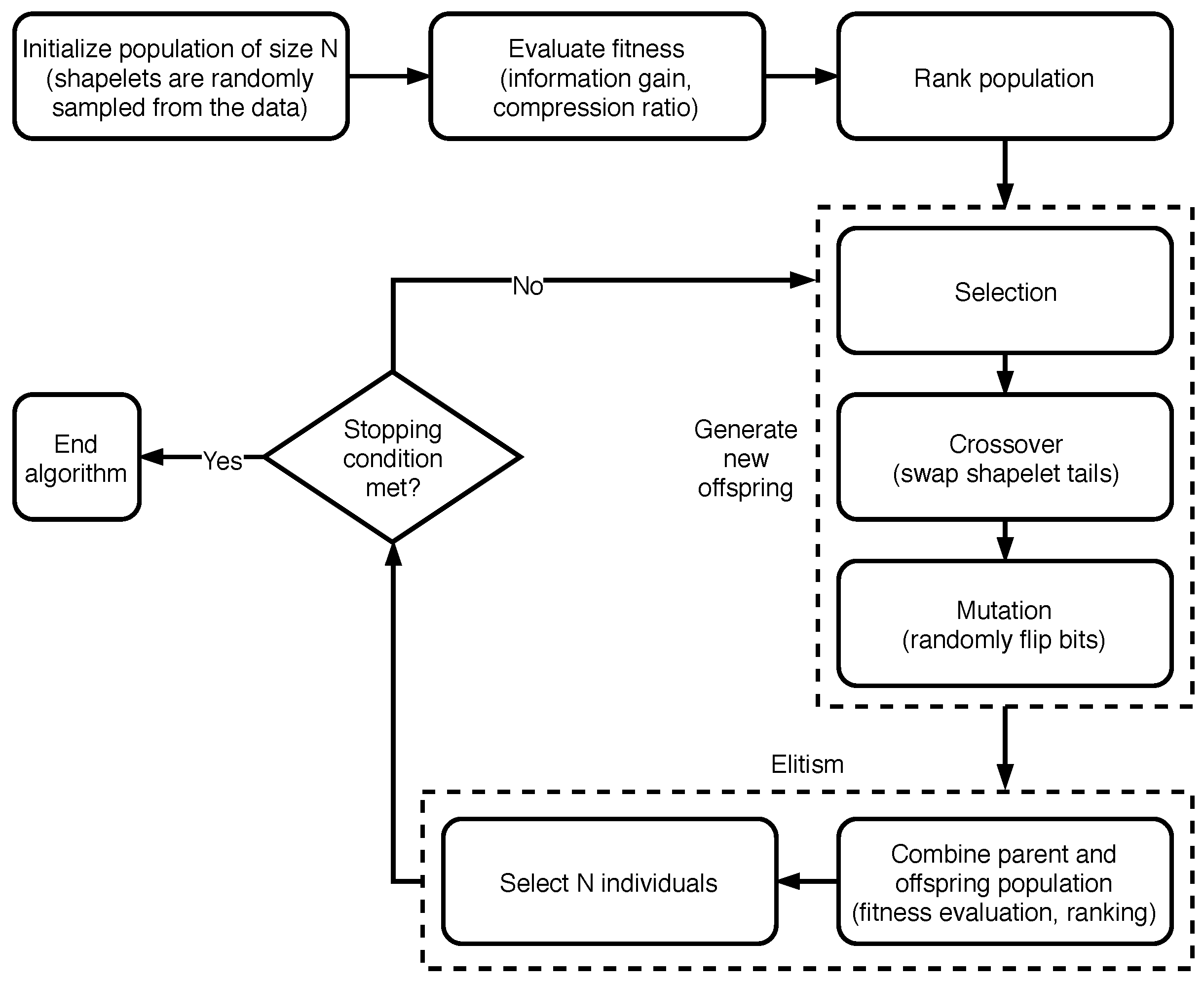
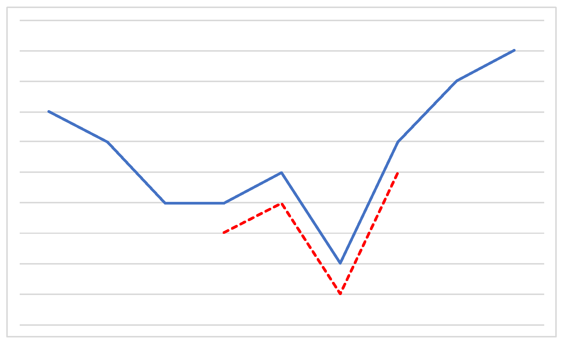
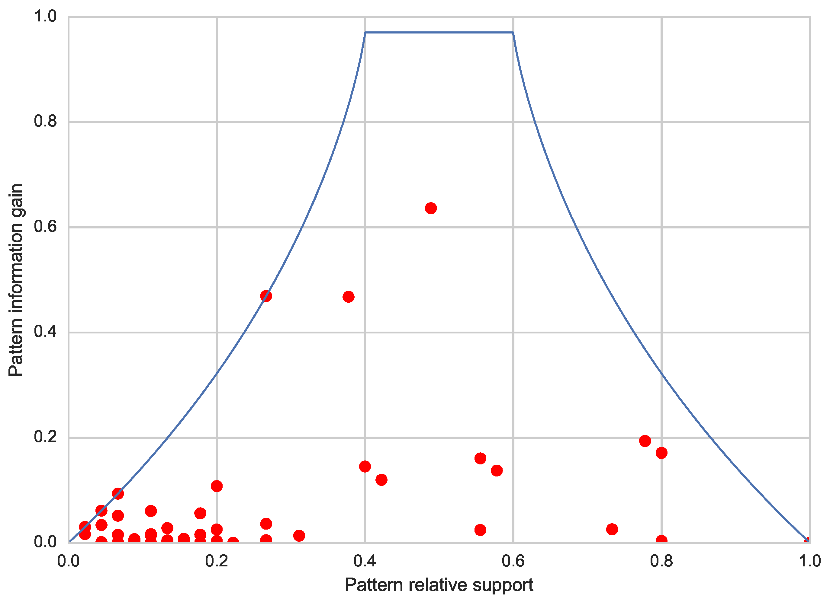
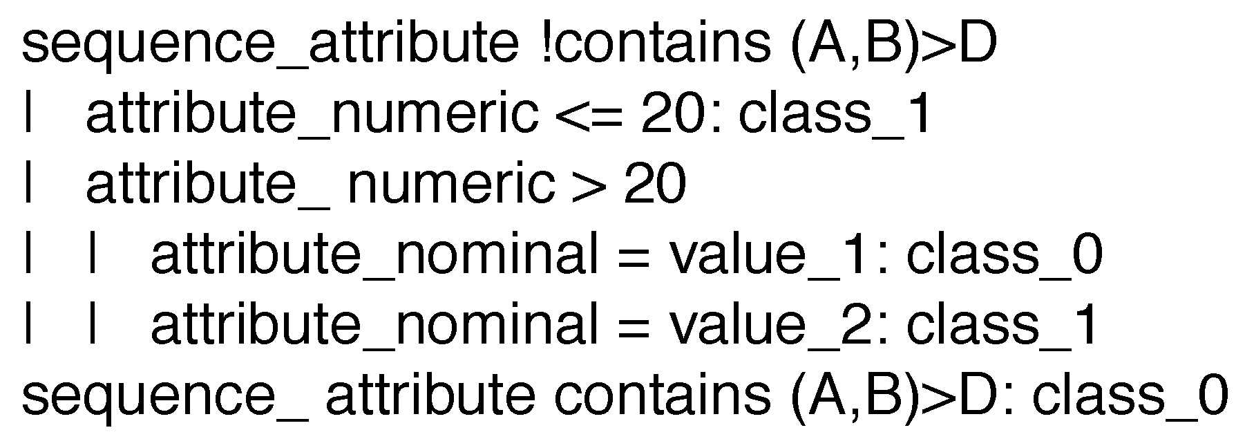
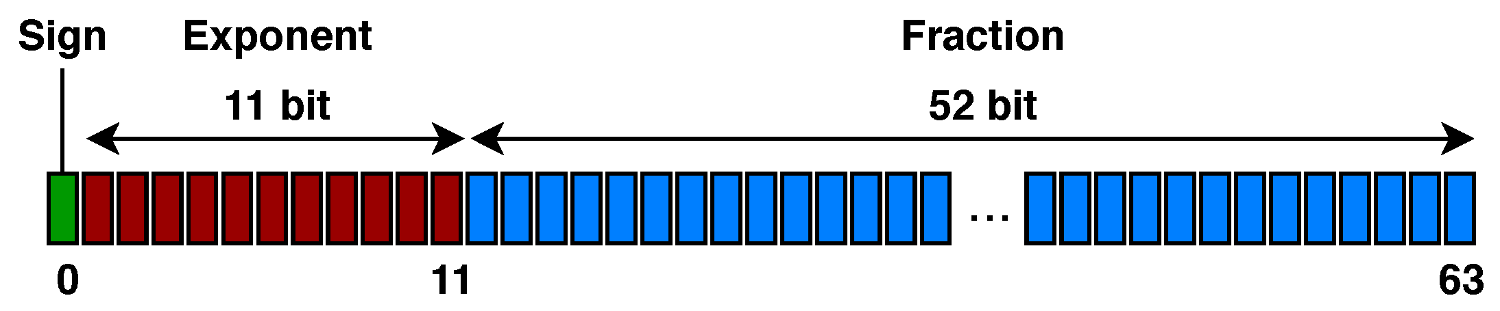
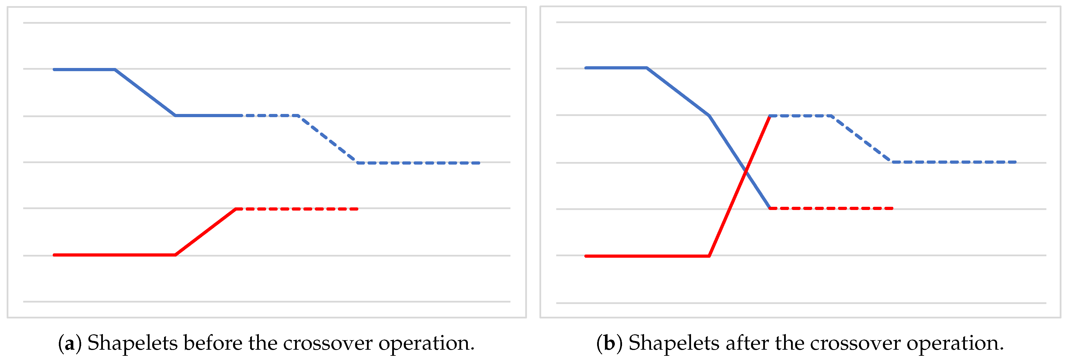
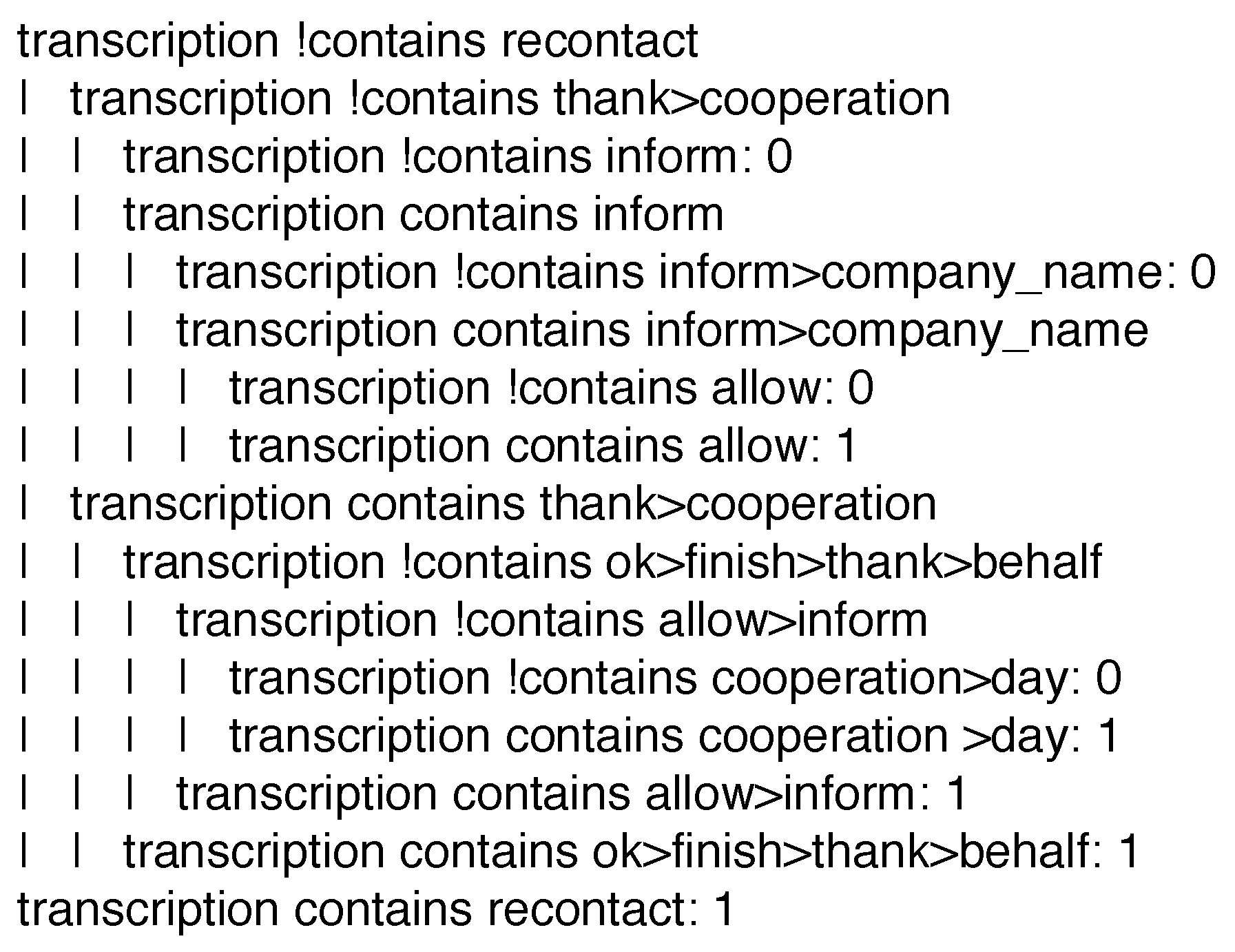
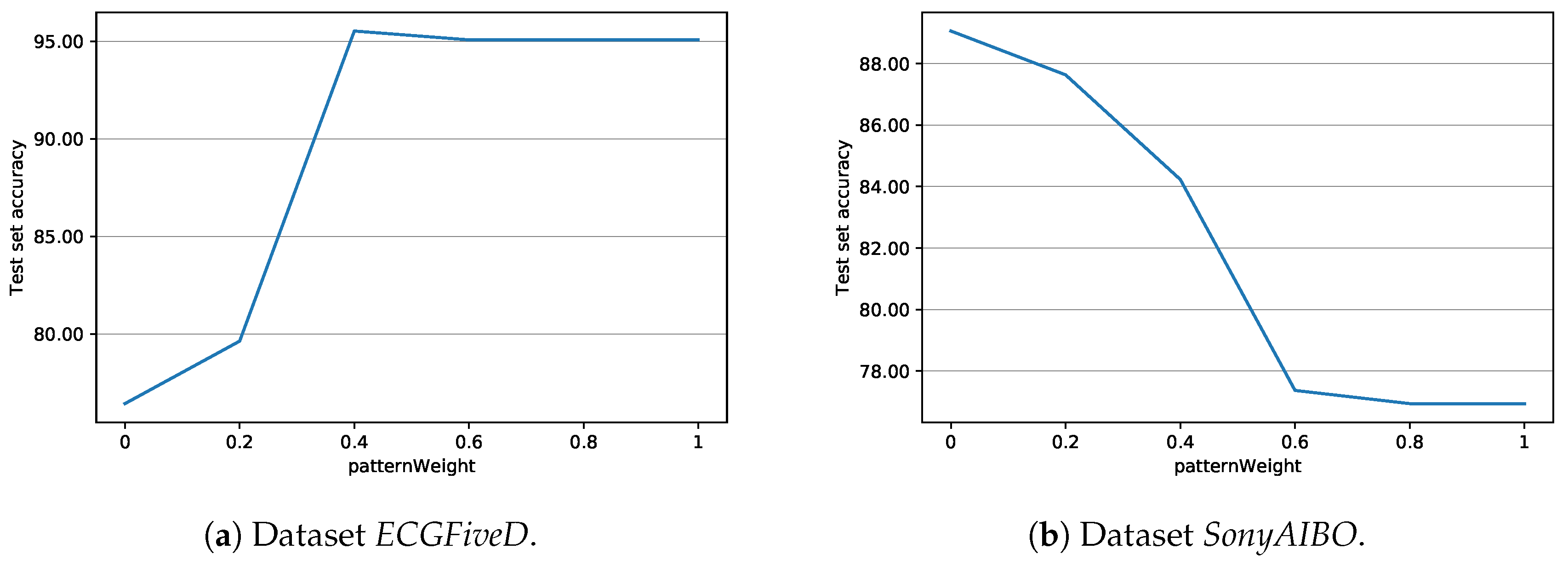
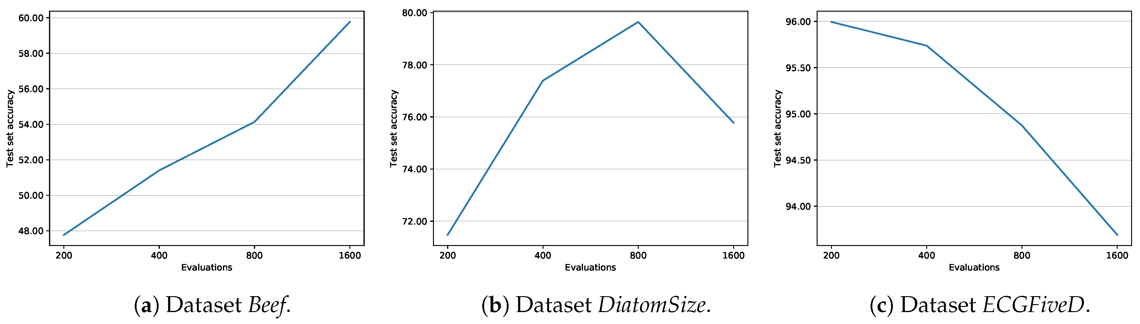
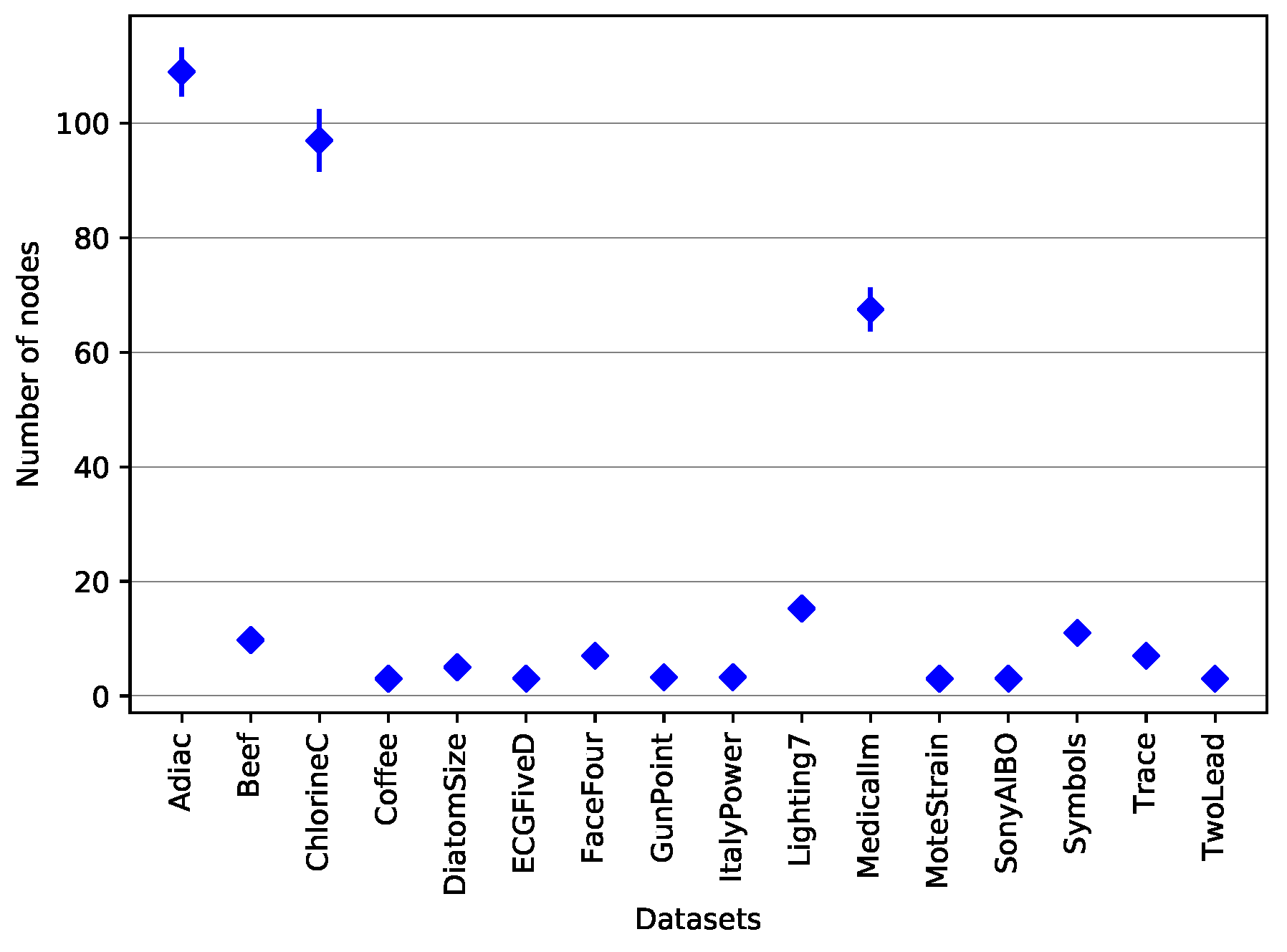
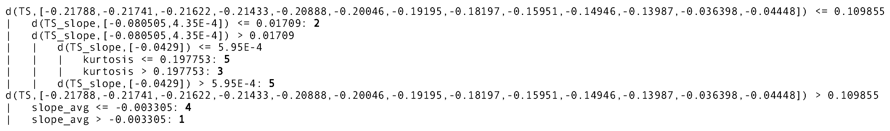
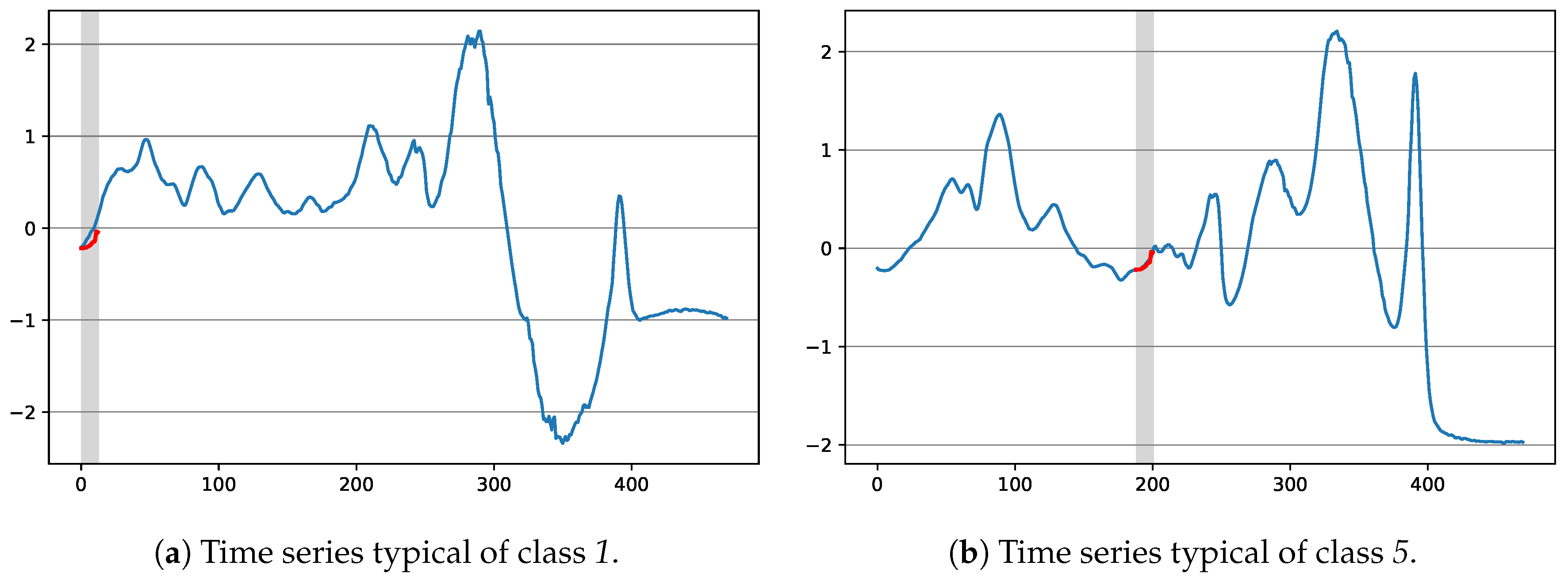
Table 1.
Custom parameters for sequential pattern extraction in J48SS.
| Parameter Name | Default | Description |
|---|---|---|
| maxGap | 2 | maximum gap allowance between itemsets (1 = contiguous) |
| maxPatternLength | 20 | maximum length of a pattern, in number of items |
| maxTime | 30 | maximum allowed running time of the algorithm, per call |
| minSupport | 0.5 | minimum support of a pattern |
| patternWeight | 0.5 | weight used in VGEN for the extraction of the result |
| useIGPruning | True | use information gain pruning of the pattern search space |
Table 2.
Custom Parameters for time series shapelet extraction in J48SS.
| Parameter Name | Default | Description |
|---|---|---|
| crossoverP | 0.8 | crossover probability to be used in the evolutionary algorithm |
| mutationP | 0.1 | mutation probability to be used in the evolutionary algorithm |
| numEvals | 500 | number of evaluations to be carried out by the evolutionary algorithm |
| patternWeight | 0.75 | weight used for the extraction of the final shapelet |
| popSize | 100 | population size to be used in the evolutionary algorithm |
Table 3.
Transcriptions with the associated tags. Data has been anonymized, and punctuation has been added for ease of reading.
Table 3.
Transcriptions with the associated tags. Data has been anonymized, and punctuation has been added for ease of reading.
| Phrase (Italian) | Phrase (English) | Tags |
|---|---|---|
| Si pronto buongiorno sono X dalla X di X, parlo con la signora X? | Hello, my name is X and I am calling from X of X, am I talking with Mrs X? | greeting_initial, person_identity |
| Lei è pensionato. Ultima domanda, senta, a livello statistico la data solo di nascita… millenovecento…? | You are retired. Last question, listen, statistically, the birth date only… nineteen hundred…? | age, profession |
| Ho capito. Posso chiederle il nome di battesimo? | Understood. May I ask you for your first name? | person_identity |
| Mi permette? Trenta secondi, tre domande velocissime… | May I? Thirty seconds, three quick questions… | duration_info |
Table 4.
Number and percentage of positive and negative tags.
| Tag Name | #Positive | %Positive | #Negative | %Negative |
|---|---|---|---|---|
| age | 638 | 13.1 | 4246 | 86.9 |
| call_permission | 565 | 11.6 | 4319 | 88.4 |
| duration_info | 491 | 10.1 | 4393 | 89.9 |
| family_unit | 506 | 10.4 | 4378 | 89.6 |
| greeting_initial | 560 | 11.5 | 4324 | 88.5 |
| greeting_final | 453 | 9.3 | 4431 | 90.7 |
| person_identity | 600 | 12.3 | 4284 | 87.7 |
| privacy | 440 | 9.0 | 4444 | 91.0 |
| profession | 391 | 8.0 | 4493 | 92.0 |
| question_1 | 516 | 10.6 | 4368 | 89.4 |
| question_2 | 496 | 10.2 | 4388 | 89.8 |
| question_3 | 500 | 10.2 | 4384 | 89.8 |
Table 5.
The UCR datasets under study, with the tuned values of patternWeight and numEvals.
| Dataset | Domain | ∣Train∣ | ∣Test∣ | TS Length | patternWeight | numEvals |
|---|---|---|---|---|---|---|
| Adiac | Biology | 390 | 391 | 176 | 0.4 | 800 |
| Beef | Food quality | 30 | 30 | 470 | 0.5 | 800 |
| ChlorineC | Health | 467 | 3840 | 166 | 0.9 | 800 |
| Coffee | Food quality | 28 | 28 | 286 | 0.0 | 800 |
| DiatomSize | Biology | 16 | 306 | 345 | 0.0 | 400 |
| ECGFiveD | Health | 23 | 861 | 136 | 0.4 | 200 |
| FaceFour | Image recognition | 24 | 88 | 350 | 0.5 | 200 |
| GunPoint | Motion detection | 50 | 150 | 150 | 0.8 | 800 |
| ItalyPower | Energy consumption | 67 | 1029 | 24 | 0.6 | 800 |
| Lighting7 | Weather prediction | 70 | 73 | 319 | 0.9 | 800 |
| MedicalIm | Health | 381 | 760 | 99 | 0.2 | 400 |
| MoteStrain | Signal discrimination | 20 | 1252 | 84 | 0.9 | 200 |
| SonyAIBO | Robotics | 20 | 601 | 70 | 0.2 | 200 |
| Symbols | Health | 25 | 995 | 398 | 1.0 | 800 |
| Trace | Nuclear energy safety | 100 | 100 | 275 | 0.5 | 400 |
| TwoLead | Health | 23 | 1139 | 82 | 0.7 | 200 |
Table 6.
Tagging performances of J48SS.
| Tag Name | Accuracy | Precision | Recall | TNR |
|---|---|---|---|---|
| age | 0.9655 | 0.9241 | 0.8171 | 0.9893 |
| call_permission | 0.9167 | 0.6500 | 0.6454 | 0.9532 |
| duration_info | 0.9739 | 0.9008 | 0.8516 | 0.9887 |
| family_unit | 0.9722 | 0.8779 | 0.8712 | 0.9848 |
| greeting_initial | 0.9739 | 0.9397 | 0.8195 | 0.9934 |
| greeting_final | 0.9916 | 0.9823 | 0.9328 | 0.9981 |
| person_identity | 0.9428 | 0.7851 | 0.6934 | 0.9753 |
| privacy | 0.9916 | 0.9550 | 0.9550 | 0.9554 |
| profession | 0.9840 | 0.8969 | 0.9063 | 0.9908 |
| question_1 | 0.9857 | 0.9688 | 0.9051 | 0.9962 |
| question_2 | 0.9815 | 0.9153 | 0.9000 | 0.9906 |
| question_3 | 0.9798 | 0.9237 | 0.8790 | 0.9915 |
| Macro average | 0.9716 | 0.8933 | 0.8480 | 0.9839 |
Table 7.
Tagging performance with logistic regression (unigrams).
| Keyword Name | Accuracy | Precision | Recall | TNR |
|---|---|---|---|---|
| age | 0.9663 | 0.8974 | 0.8537 | 0.9844 |
| call_permission | 0.9310 | 0.7980 | 0.5603 | 0.9809 |
| duration_info | 0.9672 | 0.9083 | 0.7734 | 0.9906 |
| family_unit | 0.9630 | 0.8929 | 0.7576 | 0.9886 |
| greeting_initial | 0.9773 | 0.9206 | 0.8722 | 0.9905 |
| greeting_final | 0.9941 | 0.9912 | 0.9496 | 0.9991 |
| person_identity | 0.9369 | 0.7500 | 0.6788 | 0.9705 |
| privacy | 0.9907 | 0.9545 | 0.9459 | 0.9954 |
| profession | 0.9874 | 0.8932 | 0.9583 | 0.9899 |
| question_1 | 0.9840 | 0.9683 | 0.8905 | 0.9962 |
| question_2 | 0.9840 | 0.9244 | 0.9167 | 0.9916 |
| question_3 | 0.9848 | 0.9417 | 0.9113 | 0.9934 |
| Macro average | 0.9722 | 0.9033 | 0.8390 | 0.9893 |
Table 8.
Comparison between the accuracy results of the Random Shapelet algorithm and J48SS. Observe that using a large sampling value in Random Shapelet typically leads to computation times orders of magnitude larger than those required by J48SS. Missing values, due to too long computation times (several weeks), are represented by asterisk characters (*).
| Dataset | Random Shapelet | J48SS | |||||||||
|---|---|---|---|---|---|---|---|---|---|---|---|
| 0.10 | 0.20 | 0.50 | 1.00 | 2.00 | 10.00 | 20.00 | 25.00 | 33.33 | 50.00 | ||
| Adiac | 45.4 | 47.7 | 49.6 | 50.6 | 51.9 | 51.6 | 51.3 | 51.7 | 50.3 | 51.8 | 60.5 |
| Beef | 40.0 | 39.3 | 36.8 | 35.5 | 33.6 | 32.4 | 31.6 | 32.0 | 31.8 | 31.2 | 55.4 |
| ChlorineC | 54.2 | 54.8 | 55.7 | 55.9 | 56.0 | 57.2 | 57.2 | 55.5 | 58.1 | * | 61.4 |
| Coffee | 69.0 | 70.3 | 73.1 | 74.1 | 76.4 | 76.9 | 78.1 | 78.3 | 78.3 | 78.3 | 100.0 |
| DiatomSize | 83.6 | 85.4 | 82.5 | 80.5 | 78.6 | 77.4 | 79.5 | 79.8 | 79.9 | 79.7 | 82.7 |
| ECGFiveD | 94.2 | 96.2 | 96.7 | 97.2 | 97.3 | 97.7 | 97.3 | 97.0 | 96.7 | 96.1 | 96.2 |
| FaceFour | 72.1 | 71.6 | 73.8 | 72.9 | 72.8 | 74.2 | 74.6 | 75.0 | 75.5 | 74.4 | 84.5 |
| GunPoint | 89.3 | 88.3 | 87.9 | 87.3 | 87.3 | 84.4 | 82.9 | 82.7 | 82.8 | 82.9 | 91.8 |
| ItalyPower | 87.1 | 87.8 | 90.0 | 90.4 | 90.8 | 92.4 | 93.0 | 93.0 | 93.1 | 93.2 | 92.7 |
| Lighting7 | 61.9 | 61.0 | 58.1 | 56.9 | 56.9 | 63.50 | 63.5 | 63.9 | 64.9 | 63.0 | 66.0 |
| MedicalIm | 58.3 | 58.5 | 58.8 | 58.9 | 58.8 | 59.2 | 59.6 | 59.8 | 59.7 | 60.6 | 65.8 |
| MoteStrain | 78.4 | 78.9 | 79.2 | 79.2 | 79.2 | 81.5 | 81.8 | 82.3 | 82.2 | 82.0 | 81.5 |
| SonyAIBO | 83.8 | 84.9 | 85.5 | 86.9 | 86.3 | 86.8 | 87.2 | 87.9 | 88.6 | 89.8 | 89.2 |
| Symbols | 78.0 | 76.1 | 76.0 | 75.2 | 76.8 | 79.5 | 80.6 | 80.8 | 80.7 | 80.6 | 77.6 |
| Trace | 94.4 | 94.5 | 95.0 | 95.0 | 94.6 | 93.4 | 93.1 | 93.1 | 93.0 | 93.0 | 95.0 |
| TwoLead | 82.2 | 85.6 | 87.4 | 89.5 | 90.2 | 91.4 | 92.1 | 92.1 | 92.1 | 92.0 | 90.6 |
| Average | 73.2 | 73.8 | 74.1 | 74.1 | 74.2 | 75.0 | 75.2 | 75.3 | 75.5 | N/A | 80.7 |
Table 9.
Average of J48SS training times (in seconds), considering different numbers of evaluations of the evolutionary algorithm.
Table 9.
Average of J48SS training times (in seconds), considering different numbers of evaluations of the evolutionary algorithm.
| Dataset | 200 Evals | 400 Evals | 800 Evals | 1600 Evals |
|---|---|---|---|---|
| Adiac | 14.1 | 20.8 | 37.8 | 98.9 |
| Beef | 3.7 | 5.2 | 7.72 | 14.8 |
| ChlorineC | 24.5 | 30.1 | 44.2 | 86.4 |
| Coffee | 1.1 | 1.4 | 2.0 | 4.0 |
| DiatomSize | 1.9 | 2.5 | 4.1 | 10.9 |
| ECGFiveD | 0.8 | 1.1 | 1.4 | 2.2 |
| FaceFour | 2.1 | 2.8 | 4.3 | 8.2 |
| GunPoint | 1.3 | 1.5 | 1.9 | 2.6 |
| ItalyPower | 0.8 | 0.9 | 1.3 | 2.4 |
| Lighting7 | 4.6 | 6.6 | 10.2 | 18.6 |
| MedicalIm | 8.3 | 11.0 | 17.4 | 38.4 |
| MoteStrain | 0.6 | 0.7 | 0.9 | 1.3 |
| SonyAIBO | 0.6 | 0.8 | 1.0 | 1.9 |
| Symbols | 2.7 | 3.9 | 6.3 | 14.5 |
| Trace | 2.2 | 3.0 | 4.6 | 9.5 |
| TwoLead | 0.5 | 0.7 | 0.9 | 1.5 |
Table 10.
Comparison between accuracy and training time (in seconds) of EJ48SS (100 trees), and Generalized Random Shapelet Forests (500 trees).
Table 10.
Comparison between accuracy and training time (in seconds) of EJ48SS (100 trees), and Generalized Random Shapelet Forests (500 trees).
| Dataset | gRSF Accuracy | EJ48SS Accuracy | EJ48SS Training Time (s) |
|---|---|---|---|
| Adiac | 74.2 | 78.1 | 2196.8 |
| Beef | 80.0 | 67.5 | 269.1 |
| ChlorineC | 67.3 | 72.2 | 2230.9 |
| Coffee | 100.0 | 100.0 | 49.0 |
| DiatomSize | 96.4 | 86.8 | 57.6 |
| ECGFiveD | 100.0 | 100.0 | 6.2 |
| FaceFour | 100.0 | 92.8 | 36.8 |
| GunPoint | 100.0 | 98.0 | 40.2 |
| ItalyPower | 94.0 | 95.6 | 19.3 |
| Lighting7 | 69.9 | 73.1 | 410.5 |
| MedicalIm | 73.3 | 75.5 | 392.2 |
| MoteStrain | 92.1 | 92.6 | 6.5 |
| SonyAIBO | 92.5 | 90.4 | 6.4 |
| Symbols | 96.8 | 76.1 | 215.2 |
| Trace | 100.0 | 99.1 | 61.5 |
| TwoLead | 100.0 | 97.1 | 5.8 |
| Average | 89.8 | 87.2 |
© 2019 by the authors. Licensee MDPI, Basel, Switzerland. This article is an open access article distributed under the terms and conditions of the Creative Commons Attribution (CC BY) license (http://creativecommons.org/licenses/by/4.0/).
Share and Cite
MDPI and ACS Style
Brunello, A.; Marzano, E.; Montanari, A.; Sciavicco, G. J48SS: A Novel Decision Tree Approach for the Handling of Sequential and Time Series Data. Computers 2019, 8, 21. https://0-doi-org.brum.beds.ac.uk/10.3390/computers8010021
AMA Style
Brunello A, Marzano E, Montanari A, Sciavicco G. J48SS: A Novel Decision Tree Approach for the Handling of Sequential and Time Series Data. Computers. 2019; 8(1):21. https://0-doi-org.brum.beds.ac.uk/10.3390/computers8010021
Chicago/Turabian StyleBrunello, Andrea, Enrico Marzano, Angelo Montanari, and Guido Sciavicco. 2019. "J48SS: A Novel Decision Tree Approach for the Handling of Sequential and Time Series Data" Computers 8, no. 1: 21. https://0-doi-org.brum.beds.ac.uk/10.3390/computers8010021
Note that from the first issue of 2016, this journal uses article numbers instead of page numbers. See further details here.