The Use of an Artificial Neural Network to Process Hydrographic Big Data during Surface Modeling †


Institute of Geoinformatics, Faculty of Navigation, Maritime University of Szczecin, 70-500 Szczecin, Poland
*
Author to whom correspondence should be addressed.
†
This paper is an extended version of our conference paper: Lubczonek, J.; Wlodarczyk-Sielicka, M. The Use of an Artificial Neural Network for a Sea Bottom Modelling. In Proceedings of the 24th International Conference on Information and Software Technologies (ICIST 2018), Vilnius, Lithuania, 4–6 October 2018.
Computers 2019, 8(1), 26; https://0-doi-org.brum.beds.ac.uk/10.3390/computers8010026
Submission received: 30 January 2019
/
Revised: 5 March 2019
/
Accepted: 11 March 2019
/
Published: 14 March 2019
(This article belongs to the Special Issue Selected Papers from the 24th International Conference on Information and Software Technologies (ICIST 2018))
Abstract
:At the present time, spatial data are often acquired using varied remote sensing sensors and systems, which produce big data sets. One significant product from these data is a digital model of geographical surfaces, including the surface of the sea floor. To improve data processing, presentation, and management, it is often indispensable to reduce the number of data points. This paper presents research regarding the application of artificial neural networks to bathymetric data reductions. This research considers results from radial networks and self-organizing Kohonen networks. During reconstructions of the seabed model, the results show that neural networks with fewer hidden neurons than the number of data points can replicate the original data set, while the Kohonen network can be used for clustering during big geodata reduction. Practical implementations of neural networks capable of creating surface models and reducing bathymetric data are presented.
1. Introduction
Surface modeling has been the subject of various prior studies [1,2], but these have focused largely on numerical methods. Mathematical formulas and sample data sets were mainly used during the surface reconstruction process. Surfaces created as raster models are currently used in many tasks, especially in geographic information systems, which are based on digital geographical surface processing [3]. Artificial neural networks, which are widely used in many applications, can also be applied to this task. One such application is to marine tasks, including ship positioning [4], data association for target tracking [5], or seabed model building [6,7,8]. At present, various types of neural networks are used to solve these tasks, such as radial networks, self-organizing networks, and multilayer perceptrons. One property of neural networks which is applicable to surface modeling is their ability to functionally approximate many variables. However, nowadays, data are collected in sets of up to as many as a million points using new remote sensing technics, such as light detection and ranging, photogrammetry, radar interferometry, and multibeam echo sounding. Bathymetric geodata gathered by the usage of modern hydrographic systems consists of a very large set of measuring points. It is associated with long-lasting and labor-intensive data processing. The concept of a large dataset, which is bathymetric geodata, should be further clarified [9]. Big data refers to large, variable, and diverse data sets, the processing and analysis of which is difficult, but also valuable, because it can lead to new knowledge. It can be stated that the concept of a large data set is associated with the difficulty of their rational utilization using commonly available methods [10]. Even for the numerical methods used in the process of surface creation, such big data sets are problematic to process. An obvious solution to this issue would be to apply data reduction so that a minimum quantity of points would be sufficient for surface restoration within specified tolerance limits. However, the application of neural networks could allow this problem to be solved a different way. By properly adjusting the neural network framework, the number of elements, such as layers or neurons, can be reduced. Using this approach, a smaller data set representing the neural network structure could substitute the original, larger data set of measurement points. An alternative approach might involve the reduction of the number of measuring samples. This manuscript shows that it is possible to use radial and self-organizing networks to achieve the above aims.
The paper is ordered as follows: Section 2 describes the test surfaces used, which reflect the shape of the seabed, and the optimization of neural networks used during the studies; Section 3 describes the methodology of the analyses conducted and experimental results with a discussion, ending with conclusions.
2. Methods
This section describes the characteristics of the test surfaces used for this research, and artificial neural network optimization for bathymetric geodata modeling.
2.1. Surfaces Used During the Tests
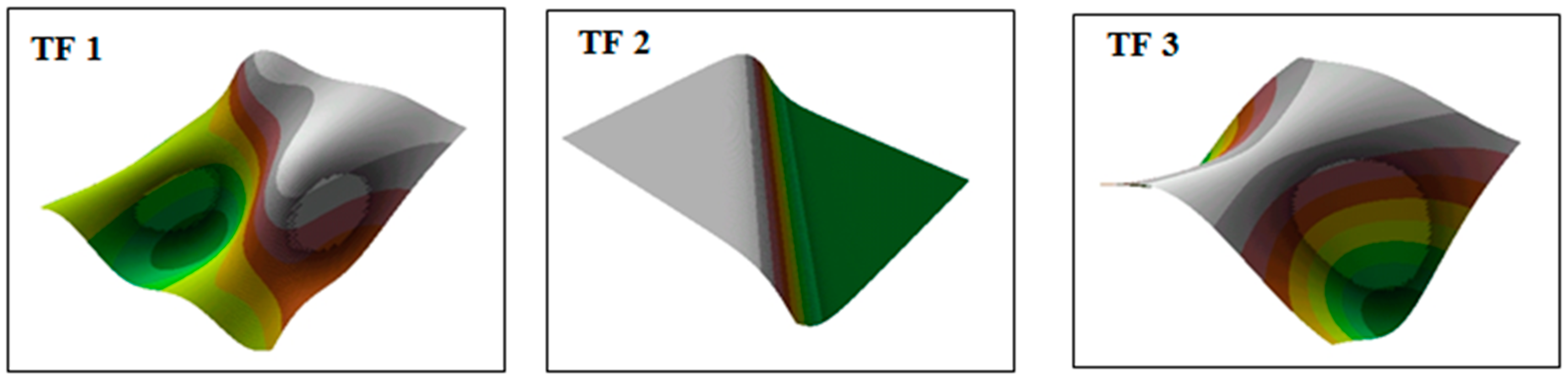
Numerical experiments were based on three surface kinds which depict various forms of real seabed surfaces. The miscellaneous surface shapes allowed the performance of this method to be assessed for various degrees of surface curvature. The test surfaces were formed using three test functions, denoted as TF:
Finally, after rescaling by 100, the range of the surface being modeled can be written as:
Surface heights (z) were also rescaled to receive greater convergence with topographical surfaces, which are metric products. The surfaces were created using test functions are showed in Figure 1.
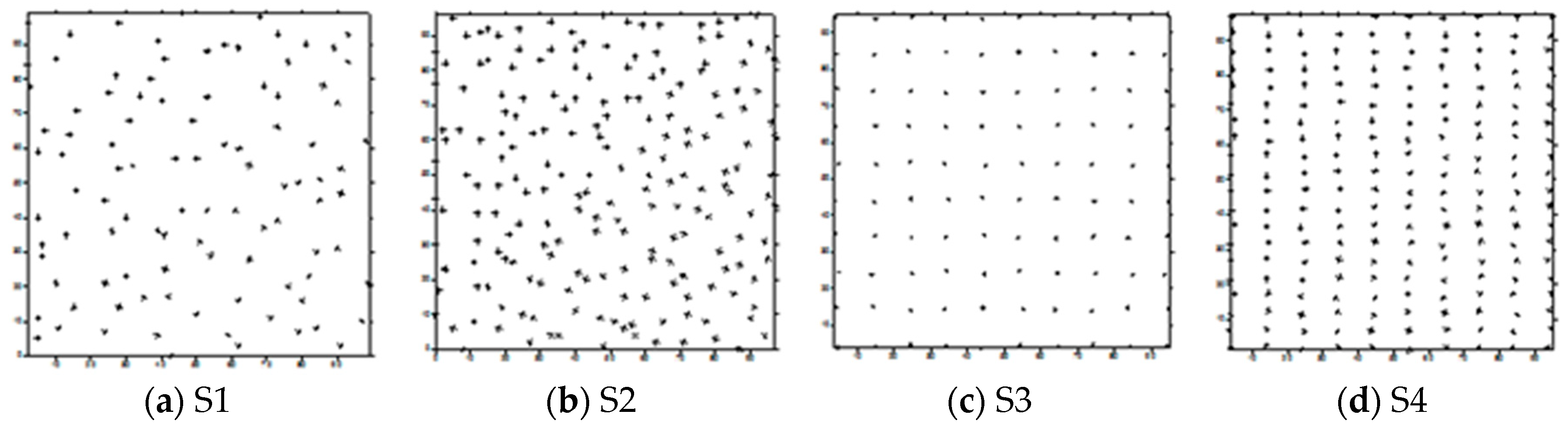
In the first part of the trial, we used four different data sets. There were two types of spatial distribution of data samples: scattered and regular. Data sets also varied in the number of points they contained: S1 = {(xi, yi): i = 1, 2, …, 100}, S2 = {(xi, yi): i = 1, 2, …, 200}, S3 = {(xi, yi): i = 1, 2, …, 100}, S4 = {(xi, yi): i = 1, 2, …, 200} and S5 = {(xi, yi): i = 1, 2, …, 200,000}. The spatial distributions of samples in S1, S2, S3, and S4 data sets are presented in Figure 2. Such distribution was determined on the basis of the real data sets, recorded by hydrographical sensors.
The spatial distribution of the S5 dataset was scattered and it contained 200,000 points. Due to high data density, this data set was not presented in the figure. In the final part of the experiment, the S5 data set for each type of the test surface was reduced.
2.2. RBF Network Optimization for Geodata Interpolation
Radial basis function (RBF) neural networks were used for the next experiment. Characteristics of RBF have been studied in a lot of reports which focus on surface shape modeling, firstly with numerical methods [11,12], and later through the wide application of neural networks. A radial network consists of three layers: one input layer, one hidden layer, and one output layer. It also simplifies network structure optimization to estimate the number of hidden layers, and to select the transfer function type, data normalization methods, and training algorithms. For data reduction optimization, the major factors are the number of neurons in hidden layer and the weights. With fewer hidden neurons, less data are required to recover the network structure.
The radial neural network approximation function can be expressed according to the following function [13,14]:
where φi is the ith radial basis function, K is the number of radial basis functions, Wi is the weight of the ith network, x is the input vector, and ti is the center of the ith RBF.
Having p data samples (x, y, z), the weights vector W can be computed by solving a system of linear equations:
where:
When the number of hidden neurons is equal to the number of training data points, the network can be used as an interpolation function, i.e., exact solution. By decreasing the number of hidden neurons, the neural network becomes an approximation; thus, we can expect some losses during surface reconstruction. On the other hand, data loss can be accepted within some specified tolerance limits. In order to estimate the influence of hidden neuron numbers on data loss experimentally, the RBF neural network with structure and training algorithms presented in Table 1 were studied.
In the case of the RBF function, the selection of radial functions is important. The most commonly used radial functions include the following: multiquadric (MQ) (11), inverse multiquadric (IMQ) (12), Duchon Thin Plate Splines (13), Gaussian (14), cubic (15), and linear (16).
Other radial functions can also be used for surface modeling, such as the Parzen function, which is used in probabilistic networks [15]
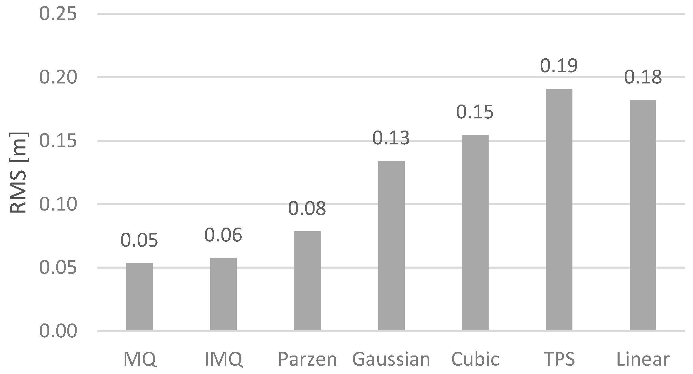
To illustrate the effect that each type of radial function has on the accuracy of surface reconstruction, the root mean square errors (RMS) were calculated for an exact solution, using initial data processing performed according to the formula:
Based on the resulting error values (Figure 3), it can be concluded that the highest surface reconstruction accuracy can be achieved using the MQ and IMQ basis functions. The average errors for the MQ, IMQ, Parzen, and Gaussian basis functions were 0.05, 0.06, 0.08, and 0.13 m, respectively. These differ from the cubic, Duchon’s TPS, and linear basis functions, which had much higher values: 0.17, 0.19, and 0.18 m, respectively. It should be clearly emphasized that in the case of the MQ, IMQ, Parzen, and Gaussian functions, small error values were achieved by optimizing the radius of basis functions, which enabled the model surface to be accurately adjusted to the set of measured points. Unfortunately, this option was not available for other basis functions, which therefore translated into a higher RMS error. The RMS error in the studies is a measure of the accuracy of surface mapping accuracy. The calculations were carried out for values located in grid nodes with a resolution of 1 m relative to the mathematical test surfaces.
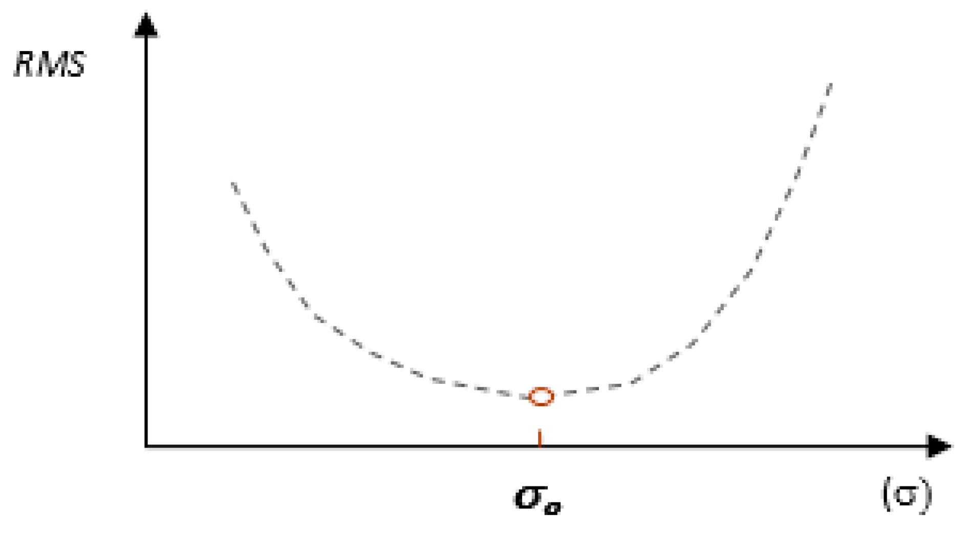
An important aspect of model fitting is the optimization of the radius of the radial function, a topic which was also the subject of previous research [16,17]. In order to minimize the RMS error, a method for optimizing the radius of the radial function has been developed. To optimize this parameter, the fact that the optimal radius of the radial function corresponds to the minimum surface reconstruction error is used [17]. Generalizing the dependence of the RMS error on the radius value of the base functions, it can be stated that as the value of the radius increases, its value decreases, then it reaches the minimum and then increases (Figure 4) There are, however, exceptions to this rule, because in the case of a characteristic data structure, the optimal value of this parameter can reach a value close to zero [11].
In this study, to optimize the radial basis function in the RBF hidden layer, an algorithm was applied which automates this process, based on the cross validation and leave-one-out (LOO) method [18].
The algorithm uses a two-step method. In the first step, a coarse radius (σz) is calculated for the basis functions based on an independent test set to minimize the RMS error, which can be treated as an approximate solution. For this step, finding a coarse value for the basis function radius was not time-consuming, because only one test set was used. The RMS error is then calculated for different values of the basis function radii, until it reaches its smallest value (these values of the radii are increased iteratively by a small interval, starting from any small value). In the second step, the radius value is computed using the more accurate but time-consuming LOO method; however, the search for the optimal value starts at the value determined from the approximate, coarse solution (σz). If we denote the error for a single-element validation set as ei, then the error for the LOO (EL) method can be calculated according to the formula:
where N is the number of measured points in the training set.
Having calculated the error in this way, by iteratively changing the value for the radius of RBF in the direction which minimized EL, the optimal value was determined. Calculation of the optimal value of the radius of the basis functions was carried out in several stages.
Stage 1. In this stage an independent test field was created using self-organizing networks constituting 15% of the number of training data points. The set was evenly distributed in the domain of the modeled surface by using self-organizing networks, with each test point selected on the basis of the smallest distance to their neurons. The amount of hidden neurons was equal to 15% of the amount of data set points. In order to better divide the entrance space, a mechanism of neuron fatigue was used, which improved the organization of the network. When self-organizing algorithms are applied, the number of wins per individual neuron are not taken into account. It can create a situation in which there is a group of neurons with a small degree of activation which will never be able to win the competition and are therefore excluded from the adaptation process. The function of the neuron fatigue mechanism is to exclude the most active neurons from the organization process for the majority of the time, which gives an opportunity for the scaling to be adapted to the remaining neurons.
The exclusion of neurons during training is accomplished by introducing a potential, pi, for each neuron, which changes across k iterations. The minimal potential, pmin, determines whether a neuron participates in the competition. Changes in neuron potentials can be calculated according to the dependency [19]:
where w designates the index of the winning neuron.
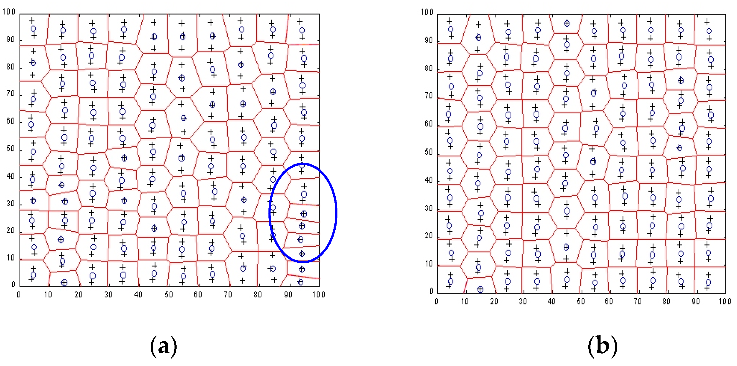
Based on the experiments that were carried out, the utility of the neuron fatigue mechanism was particularly noticeable during the organization of neurons to profile data sets. This is illustrated with graphical examples in Figure 5, in which the division of the S4 collection space (200 points) into data clusters for 100 neurons is presented using the k-means algorithm, with or without application of the neuron fatigue mechanism. Neurons that were not organized in a proper manner during learning are marked with an ellipse.
Stage 2: Calculation of RMSi errors for the polygon generated from the test samples for an algorithmically ordered set of different σi parameter values (these values are sorted in ascending order and then incremented by any small interval).
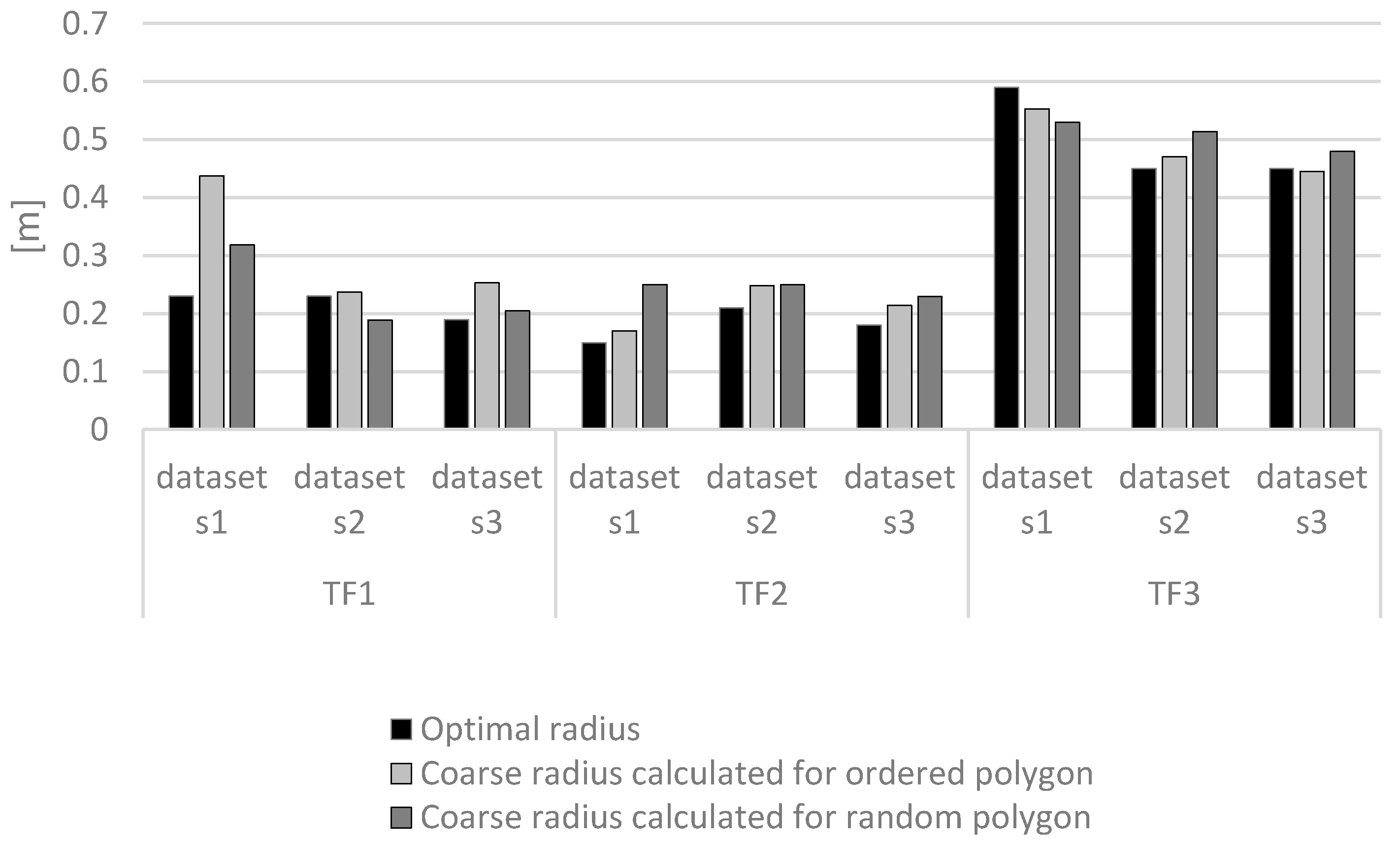
Stage 3: Determination of the coarse σz parameter, which corresponds to the minimum error value from the set of RMSi values. An important point in the calculation is the construction of a test data polygon. In the case of the coarse σz calculation for an ordered test data polygon (built using the self-organizing network), a greater convergence to the optimal solution can be obtained than by using a random spacing of samples. Figure 6 shows the optimal σ and coarse σz for ordered and random polygons. These values represent averages for 16 network organizations. In two cases for TF1 (sets S1 and S3), better results were obtained using a random polygon for optimization. In the other cases, calculating σz algorithmically using an ordered test polygon proved to be closer to the optimum solution. This approach significantly reduced the calculation time for the next stage.
Stage 4: Calculation of the optimal radius of the basis functions using the LOO method, with the search for the optimal σ parameter starting from σz.
The algorithm presented above using the MQ basis function can also become a mixed algorithm for the selection of basis functions. This possibility occurs when the RMS error reaches the minimum value for σ = 0. In this case, the basis function (11) takes the form of a linear basis function (16). For large surface modeling, this algorithm can be implemented using a hybrid neural model structure, as presented in [18,20].
2.3. Neural Network Optimization for Geodata Reduction
In the case of big bathymetric data sets, a self-organizing Kohonen network may be used to perform data reduction. Competition among neurons supplies the basis for updating values assigned to their weights. Assuming that x is the input vector, p is the number of input samples, and w is the weight vector connected with the node l, then
Each sample of the training data set are presented to the Kohonen network in an unsystematic order. Next, the nearest neuron to the inputs is selected as the winner for the input data set. The adaptation depends on the neuron distance from the input data set. The node l is then moved some proportion of the distance between its current position and the training sample. This relation depends on the learning rate. For individual objects i, the distance between the weight vector w and the input x is estimated. After starting the competition, the node l with the closest distance is selected as the winner. In the next stage, the weights w of the winner is updated using the learning principle (24). The weight vector w for the lth node in the sth step of training is denoted as and the input vector for the ith training simple is denoted as Xi. After several iterations, a training simple is selected, and the index q of the winning node is defined as
The updated Kohonen rule is as follows [21]:
where αs is the learning rate for the sth training stage [22].
In this paper, work on this method focused on determining the optimal parameters for applying self-organizing networks to bathymetric data clustering. In the beginning, the focus was on investigating the optimal number of iterations. We focused on how to optimally select the iteration count depending on the number of given clusters. Investigations were carried out on data from areas differing in the surface shape and range of depth. Based on previous studies related to iteration, the optimal number of epochs was determined to be 200. We checked it, and our previous tests were confirmed in the case of the implemented method [23]. With more iterations, the results were unchanged, but the calculation time increased. With fewer iterations, the results were unsatisfactory at the boundaries of the areas investigated.
In the next step, we focused on two parameters: the distance between each neuron and its neighbors, and initial neighborhood size. In this case, we fully based our parameters on previous studies that were published in [24]. The distance was measured using different functions: Euclidean distance, link distance, box distance, and Manhattan distance. The initial neighborhood size parameter was set on several levels. The following evaluation criteria were applied: the time taken to perform the computations, and the points distribution in individual clusters. The following parameter values were selected for the network: distance calculation using the Euclidean function, and neighborhood size set at 10. The next step was to analyze the effects of the following competition rules on the network: The winner takes all (WTA) and the winner takes most (WTM) rules. In the first case, neural adaptation relates only to the winning neuron, and neurons that lose the competition do not change their weights. The WTM rule changes not only the winner’s weight, but also the weight of its neighbors. Investigation of these rules was carried out on the same set of data used above.
The results for the different methods across clusters were comparable. The minimum depth values for each cluster were at similar levels, being exactly the same for four clusters. The major differences occurred in clusters 2 and 9. Overall, differences ranged from 5–9 cm. For WTA, the differences between minimum and maximum depths in each cluster ranged from 0.92–1.15 m, while for WTM, they ranged from 0.90–1.14 m. The biggest difference observed between the methods was only 4 cm, which was seen for cluster 7. During tests, we also paid attention to the computation time. Computation time was shorter by about 5 seconds when the winner takes most rule was examined, compared to the WTA rule [25].
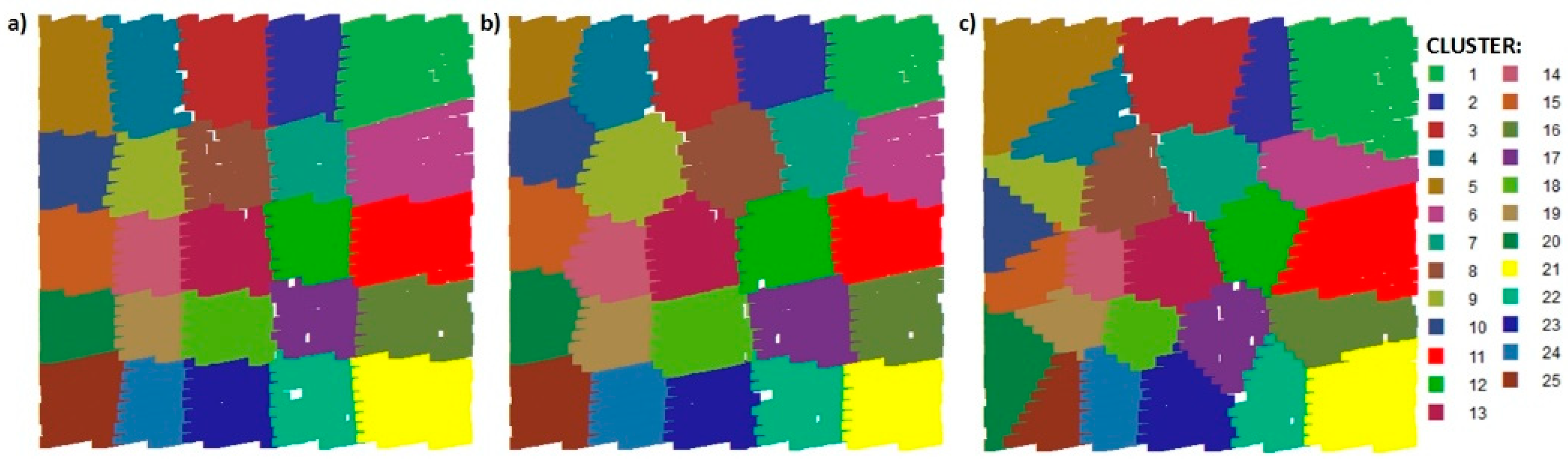
In the last step, the role played of neural network topology type during geodata clustering was analyzed. In addition to testing different types of topology, different values of the initial neighborhood size parameter were investigated again. This was necessary to check and possibly confirm whether the previously adopted value of this parameter could be applied to other types of topology. We examined the succeeding scenarios for selected parameters: grid, hexagonal, or random topology, with a neighborhood size of 1, 3, 5, or 10. One of the evaluation criteria was the calculation time, which was similar for each scenario and ranged from 14–16 s. The minimum depth for individual cluster was at a comparable level for each scenario. The biggest distinctions in depth range were observed for cluster 1. When an initial neighborhood size of 1 was used for individual topology, the spatial distribution of points was noticeably different, as shown in Figure 7.
In the case of the hexagonal topology, the results for different neighborhood sizes were almost the same [22].
After a particular analysis of all received results above for each training set, the number of epochs was set at 200. The number of training steps for initial coverage of the input space was set at 100. The network was set to apply the WTM rule and the Euclidean distance was used to calculate the distance from a particular neuron to its neighbors. The network was set to use a hexagonal topology and an initial neighborhood size of 10.
3. Results and Discussion
A series of experiments were performed on mathematical test functions. The goal of the first part of these experiments was to study the impact of hidden neuron data reduction on surface approximation error. This approach can potentially result in data reduction by replacing the real data with a lower amount of parameters which store the neural network structure. In the last stage of the test, the use of a self-organizing network for reduction and clustering of bathymetric geodata is presented.
3.1. Interpolation of Bathymetric Data
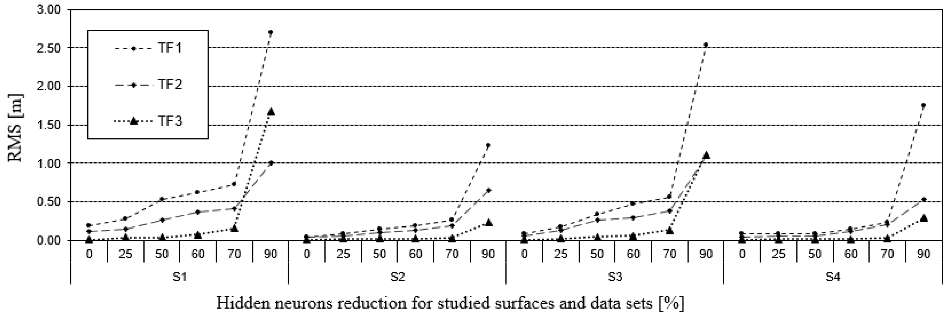
Experiments with RBF networks were conducted for two cases. At the beginning, the number of neurons in the hidden layer was set to equal the number of data points in the training set. The second case involved performing hidden neuron reductions on the training set. The initial value of hidden neurons was equal to the number of data points. Results are illustrated in Figure 8.
Analyzing the results above, we can state that the greater the reduction in hidden layer neuron numbers, the greater the increase in RMS error values. For the exact solutions, in which the number of hidden neurons is the same as the number of data points, the RMS errors have the smallest values. By further reducing the number of neurons, the RMS errors increased, but in a slightly different way for each surface type and data set. The largest RMS values were observed for TF1 and for data sets with lower data density, namely S1 and S3. These results confirm the rule that with less data for the surface creation process and a more irregular surface shape, worse results are obtained. The dependence of RMS error on hidden neuron reduction with MQ RBF for all the cases studied is presented in Figure 9.
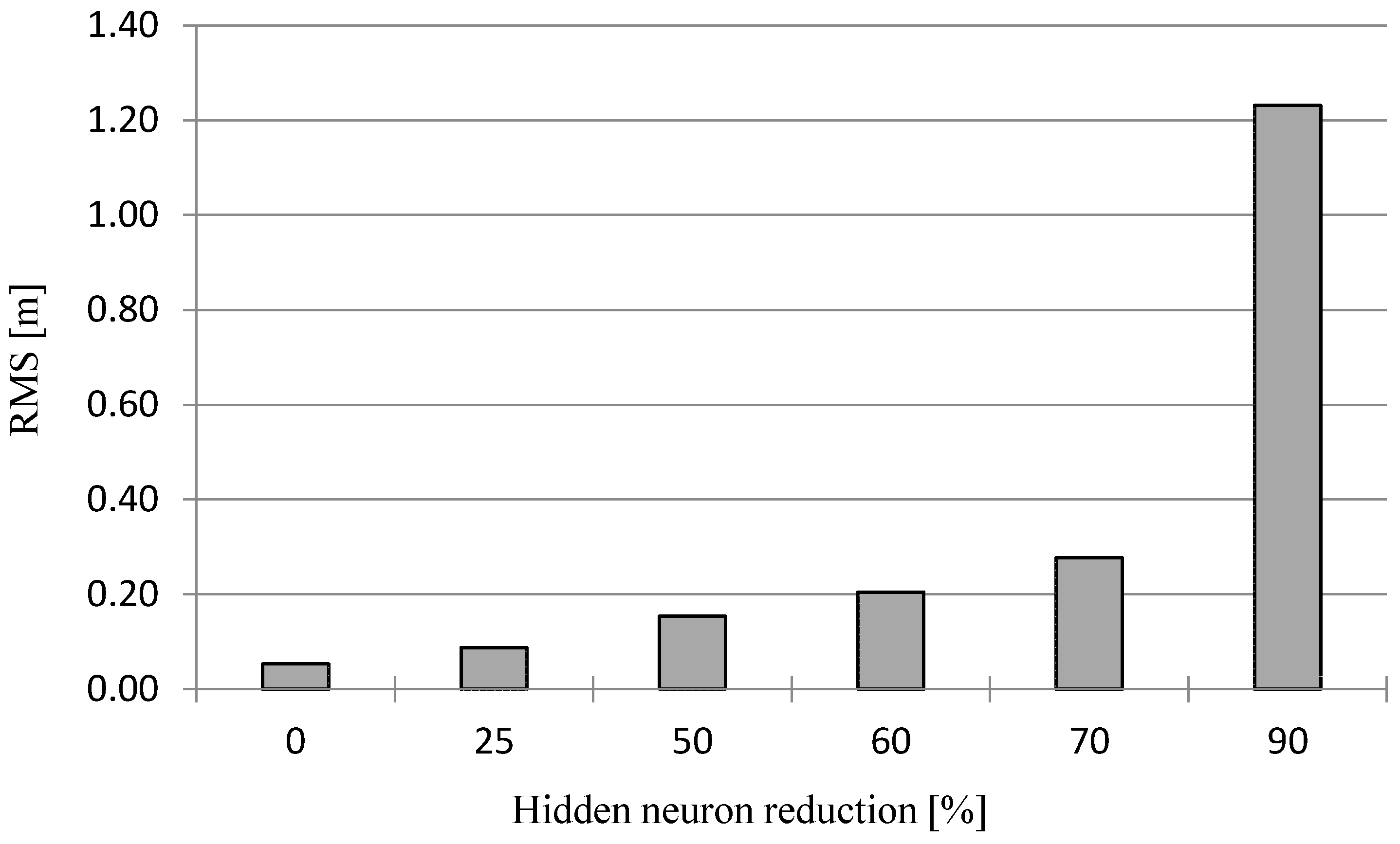
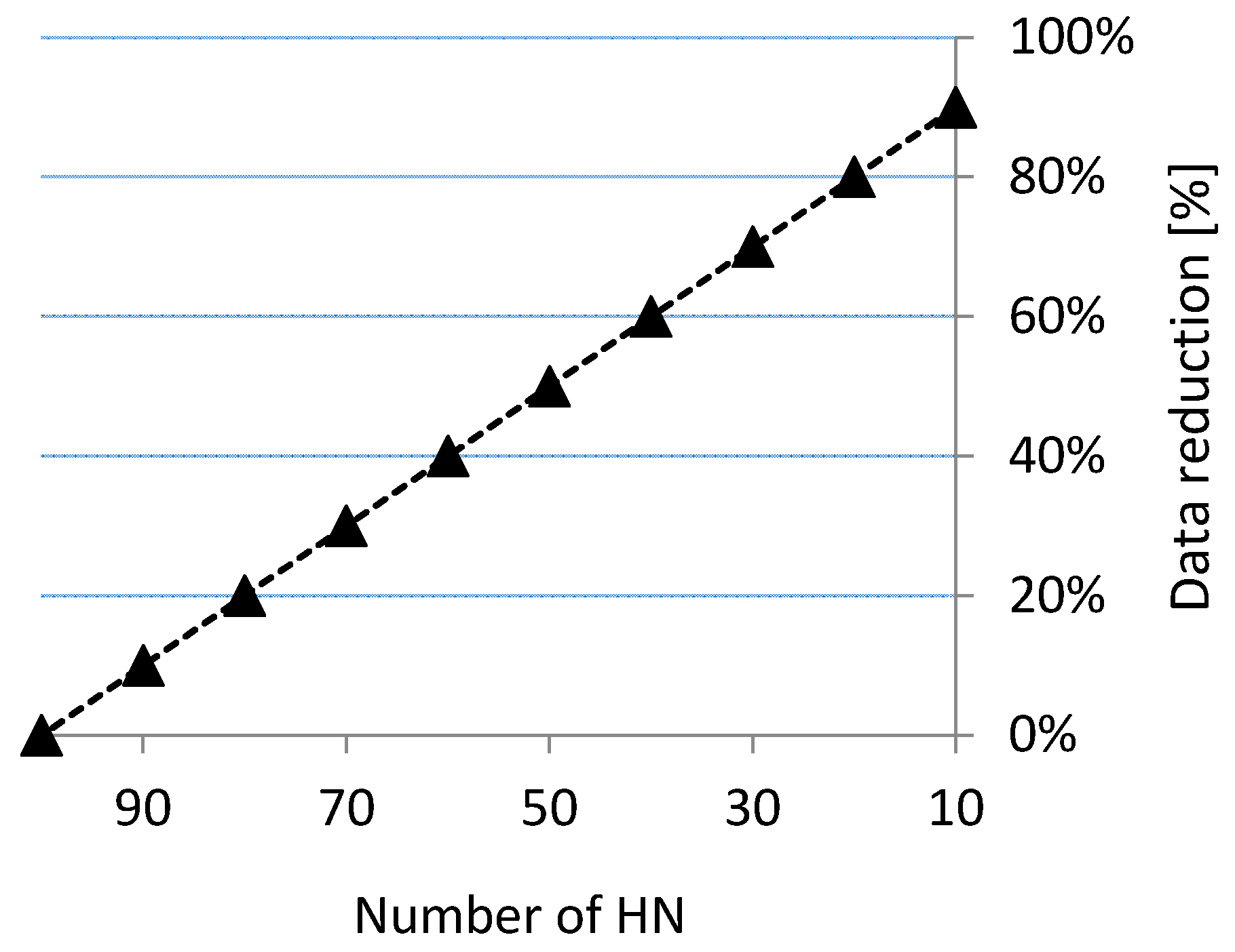
As we can note from Figure 9, RMS errors are relatively low, even for a 60% reduction in hidden neurons (0.22 m). For more generalized surfaces, the tolerance value, as a rule, is bigger, so reduction can even be applied at the level of 90%. A reduction of hidden neurons allows a decrease in the amount of data required for surface reconstruction. Comparing the amount of data required to store neural network weights to the real data set, the total data reduction can be quite large (Figure 10). For example, if the number of hidden neurons is reduced to 30, the data storage for the RBF is reduced to 70%.
It should be remembered, however, that in this case, the reconstructed surface is approximate and does not maintain the real data points.
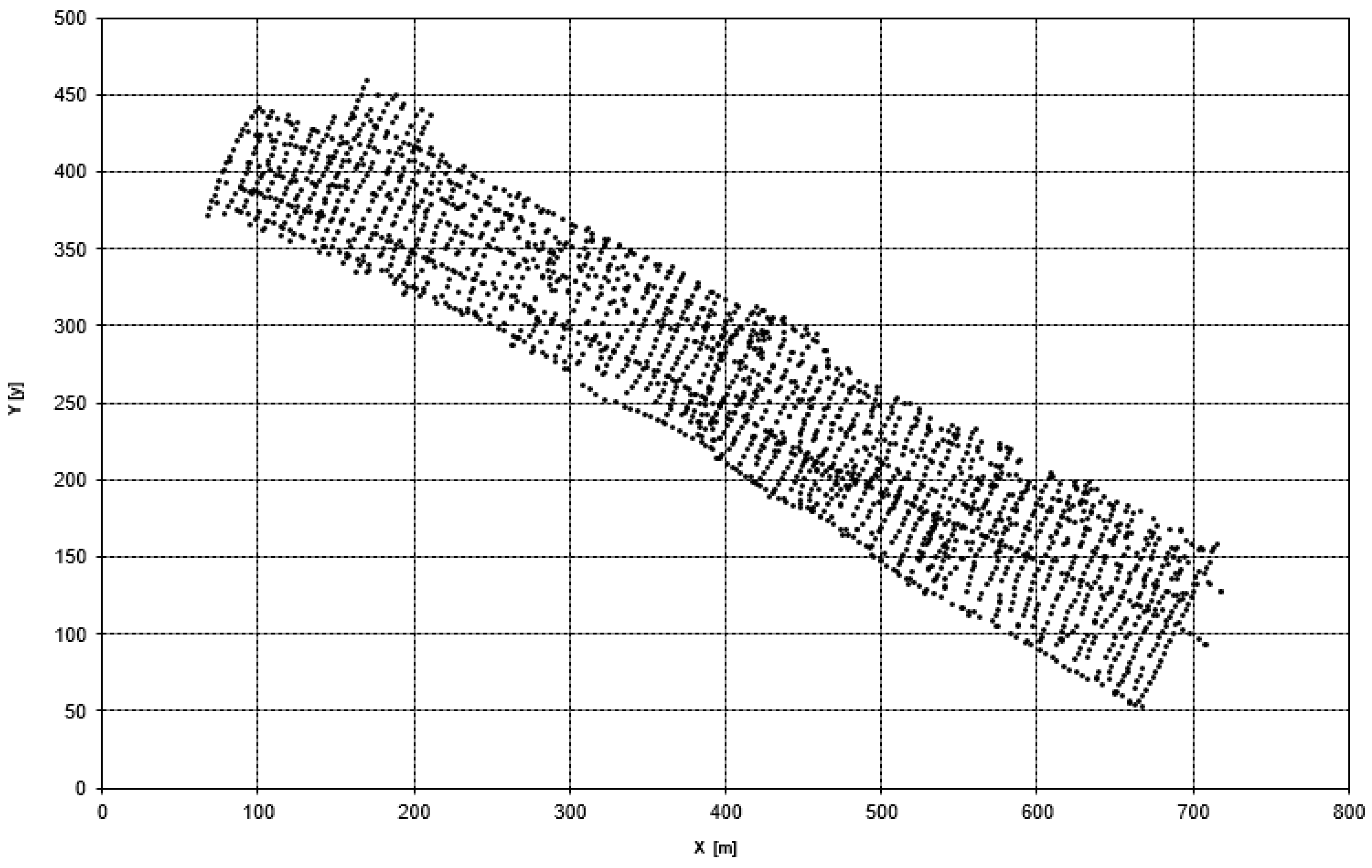
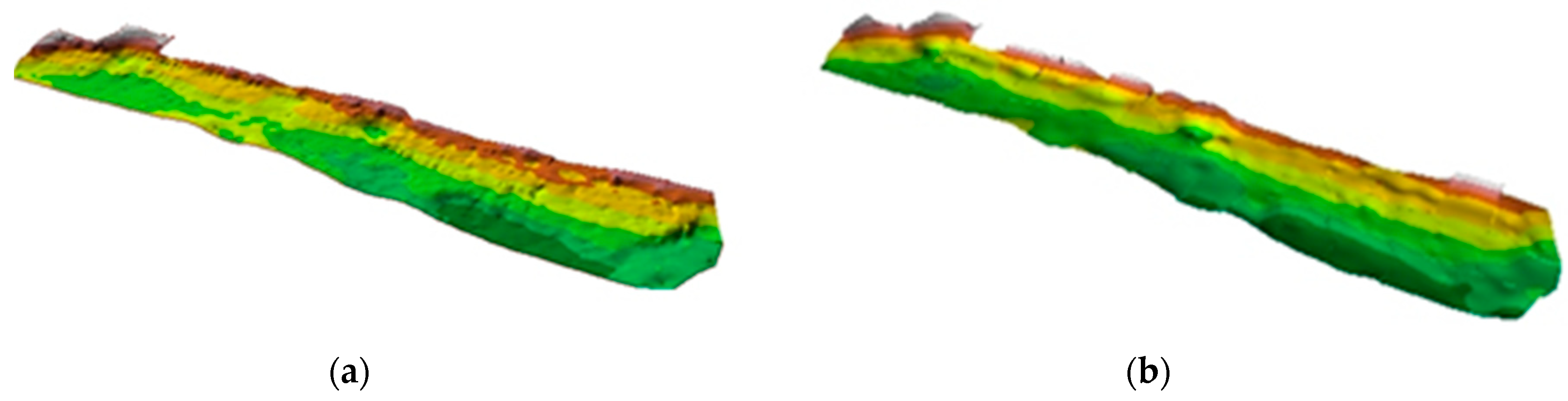
Figure 11 shows examples of surface modeling without reduction and with the reduction of hidden neurons using real data based on structure of neural model of the sea bottom [18]. Data was acquired by single beam echosounder DESO 20 in the port of Gdansk. In the case of RBF, without the reduction of hidden neurons, RMS was 0.19 m, with a reduction of up to 30 neurons at 0.21 m (Figure 12). As we can see, when reducing hidden neurons, it causes a greater generalization of the surface.
The next section describes the use of neural networks for physically-based reduction of a data set using the Kohonen network. This means that the proposed method preserves the originally measured points.
3.2. Reduction of Bathymetric Data
The next step of the experiment was to use self-organizing neural networks during the reduction of hydrographic big data sets. These investigations of reduction were carried out on the S5 dataset.
At this step, an existing reduction method was used, which was described previously in [21]. This novel method of bathymetric geodata reduction is composed of three basic stages. The first stage of the reduction method is the initial preparation of data for preprocessing. This stage is composed of two steps: preliminary division and division into grid squares. The first step, the preliminary division, is necessary in cases with large measuring areas and consists of creating data sets which are then divided into the grid squares. The grid square is based on the quad tree [26]. During the initial processing, the bathymetric data are prepared for the next stage, which involves data clustering through the use of an artificial neural network.
During this experiment, the effects of changing the values of all the parameters of the self-organizing network were analyzed: neighborhood topology and initial size, the distance function, the number of iterations, and the neuron training rule. Optimal parameter values were chosen, which led to results that fulfilled the assessment criteria. The obtained number of clusters depends on both the scale of the map and the outline of the position of each element in the geodata set [27]. Measured points from the particular clusters undergo the process of reduction, the most important being the points with the smallest depth. A circle around each point is then delineated, with its size strongly dependent on the characteristics of the tested sample. Larger circles are created around objects of greater importance so that the smaller the depth, the bigger the circle. The next step is the reduction of the points located in the circle around a point of greater importance, namely the point with the smallest depth. The process is repeated until only the circles centered on objects of greater importance are left.
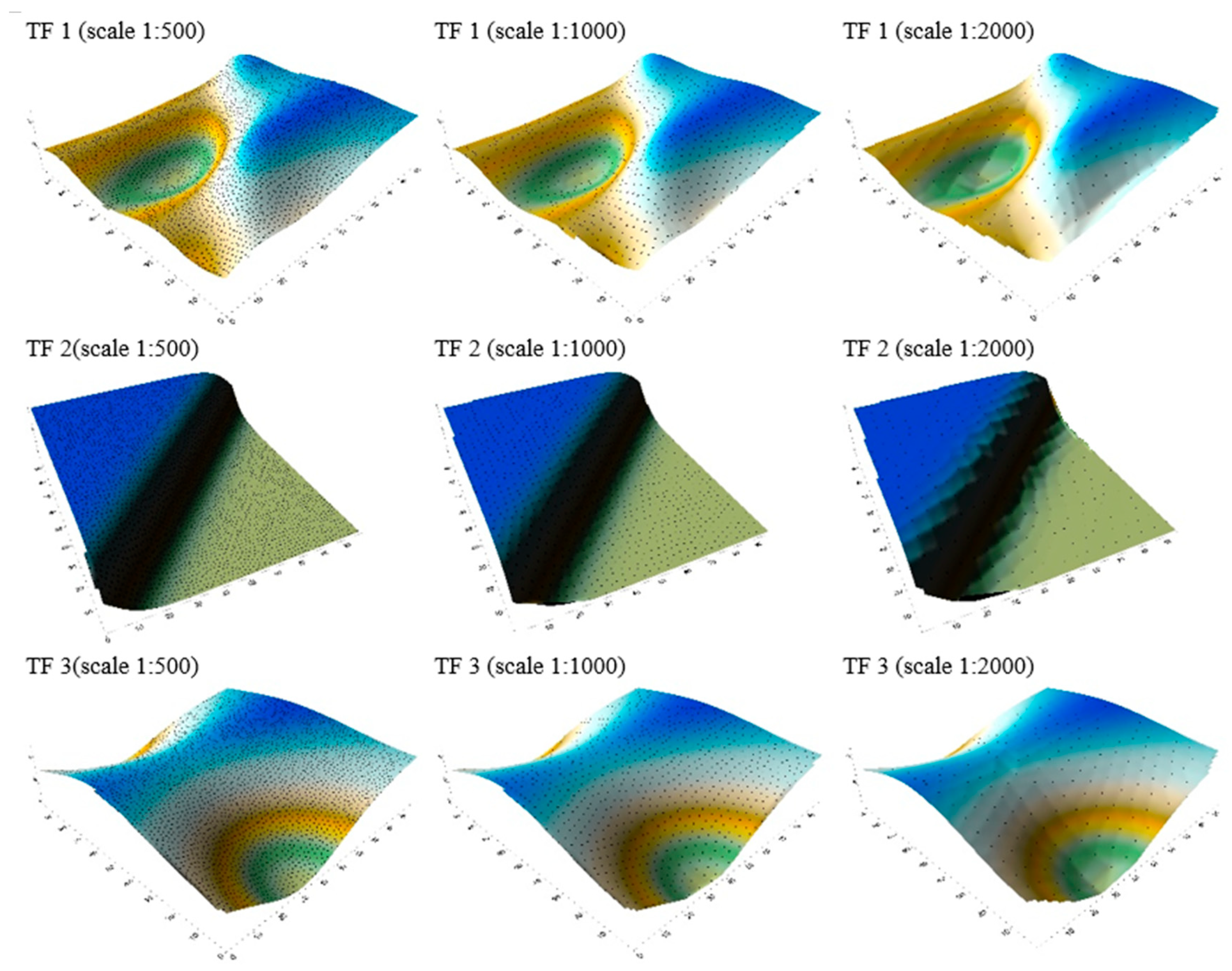
The test data set was reduced at three scales: 1:500, 1:1000, and 1:2000. To evaluate how well the novel method of bathymetric geodata reduction worked, the following criteria were taken into consideration: visual assessment of surfaces and of the distribution of obtained points; calculation of the percentage decrease in the amount of data after reduction (in other words, how much smaller is the set of points after reduction); and statistics related to the depth value.
After implementation of the chosen parameters at each scale, we obtained nine data sets after reduction. The surfaces were modeled for all the data sets using the Triangulation with Linear Interpolation method. We implemented it in the ArcGIS software package. The resulting surfaces are presented in Figure 13 with the spatial distribution of bathymetric data points shown for each scale.
Visualization of the depth points with their description showed that they fulfill the chosen evaluation criteria. The samples have been significantly reduced and their distribution is systematic. The position and depths of each point have not been interpolated. Applying the method at the 1:500 scale, the surfaces reconstructed from the remaining points almost perfectly match the shape of the test surfaces. For the other scales, the surfaces vary in their roughness, which is related to the amount of points in the dataset. However, they do not vary much from the reference surfaces, which we can see in Figure 1.
When the novel method was applied at the 1:500 scale, 97.9% of points were reduced. At the 1:1000 scale, the number of points decreased by 99.3%, and at the 1:2000 scale, the reduction was as high as 99.8%. As a result of this, analyzing and processing geodata sets becomes easier and more effective. A summary of statistics for the examined sets of samples is given in Table 2, which shows the minimum depth, maximum depth, mean depth, maximum error, and mean error.
For each reduced dataset, the smallest depth value in the test set has been preserved. As the scale decreases, the maximum and mean depth values decrease slightly. This effect is related to the number of points in the output datasets. The smallest maximum errors and mean errors were obtained for the TF3 surface, which is due to the smooth nature of its slope.
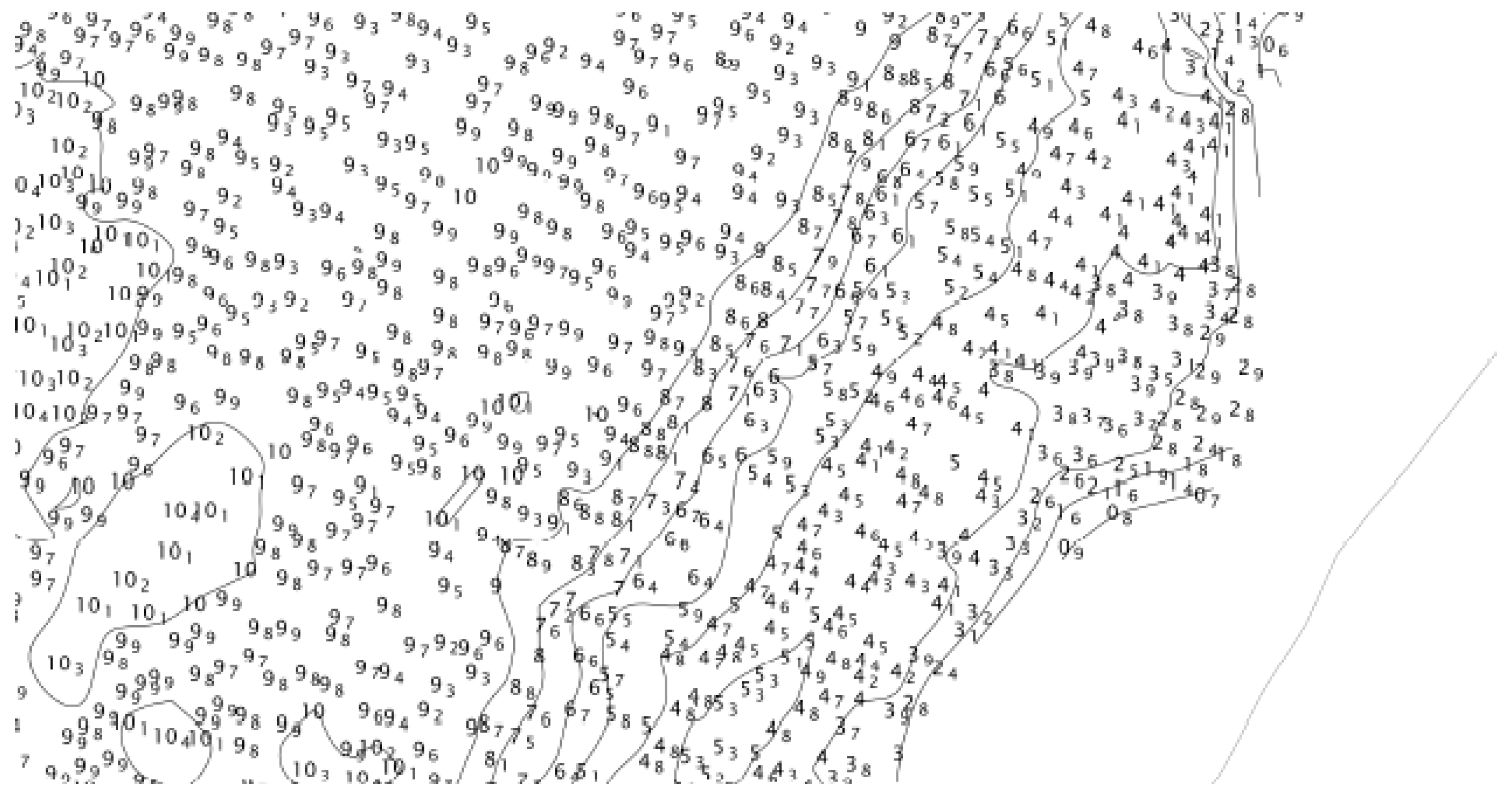
In the last step. We verified the reduction method on real data. As the main evaluation criteria, it was assumed that data after reduction should still be in the correct position and have the real depth. The second aspect assessed was the even distribution of points on the bathymetric map for a given scale and its readability. The assessed real data were gathered by the usage of GeoSwatch Plus echo sounding on the board of Hydrograf XXI laboratory. The data was collected in the Debicki canal, which is in the Szczecin port. The tested set covered an area of 10,000 m2 and contained 2,077,651 real measuring points. The minimum depth was 0.55 m and the maximum was 12 m. By using this created method, the set was reduced for three scales: 1:500, 1:1000, and 1:2000. Three sets of bathymetric geodata were obtained after reduction, which contained the following number of measuring points:
- for scale 1:500—4036 points XYZ (minimum depth 0.55 m and maximum depth 10.79 m);
- for scale 1:1000—1306 points XYZ (minimum depth 0.55 m and maximum depth 10.65 m);
- for scale 1:2000—497 points XYZ (minimum depth 0.55 m and maximum depth 10.56 m).
The collections obtained during the reduction process were used to create bathymetric maps of the reservoir. Figure 14 illustrates a section of the studied area that includes the coastal area of the Debicki canal.
It can be stated that prepared bathymetric plans fulfil the criteria of visual assessment. The novel method presented mostly concentrated on the smallest depth values, which is important for navigational safety. The use of reduction method presented makes it possible to preserve 100% of the characteristics of the surfaces.
4. Conclusions
In this manuscript, we investigated the application of artificial neural networks to seabed surface modeling. This problem is significant in current research because of the application of present-day sensors to remote sensing, which are able to gather big geodata sets. Artificial neural networks, besides offering the chance of creating surface models, can also reduce the data required for surface reconstruction. This type of reduction is based on replacing samples with data representing the neural network structure, which can require the storage of less data to reconstruct the surface. A possible alternative approach is to use neural networks for clustering, which can be part of the reduction process. This study has not considered informatics, in terms of methods of data storage and algorithm implementation, which determines the physical data size of the files.
Based on this research, it can be stated that radial neural networks are more flexible in performing surface reconstruction because they can be used as interpolators or approximators. However, in the first case, due to the exact solution, it is not possible to perform data reduction. The reduction of neurons achieved also depends on the tolerance threshold, which determines the number of hidden neurons. The Kohonen network used in the second stage of the original reduction method described above also fulfills a well-established role. The novel method of reduction presented here makes it possible to maintain the original values of depth and locations of the measured data points. The size of the bathymetric data set was greatly reduced, in close relationship to the scale of the bathymetric map. Obtained data were characterized by lower surface projection errors, which were a result of preserving the real depth values without interpolation. Points obtained from the reduction process may be implemented in the process of creating the bathymetric maps. In the case of the reduction of large datasets, we are currently focusing on navigable waters that, according to requirements, should have a coverage of 100 percent. More detailed analyses related to lower data density on steep surfaces can be the subject of further research.
In conclusion, this paper presents a series of studies performed on test functions. We used low-density data and those with very high density. The former were used to reconstruct the seabed surface, while the latter were used for data reduction. An important finding is that neural networks need an additional method, which allows them to be implemented for large surface modeling in the informatics sense. This can cause a diminished performance in terms of data reduction. This performance can vary according to the method implemented, and therefore, each case should be considered individually.
Author Contributions
conceptualization, M.W.-S. and J.L.; methodology, M.W.-S. and J.L.; software, M.W.-S. and J.L.; formal analysis, M.W.-S. and J.L.; data curation, M.W.-S. and J.L.; writing—original draft preparation, M.W.-S. and J.L.; writing—review and editing, M.W.-S. and J.L.; visualization, M.W.-S. and J.L.
Funding
This research received no external funding.
Acknowledgments
This research was completed under grants no. 1/S/IG/16 and 17/MN/IG/18, financed by a subsidy of the Ministry of Science and Higher Education for statutory activities.
Conflicts of Interest
The authors declare no conflict of interest.
References
- Franke, R. Scattered data interpolation: Test of some methods. Math. Comput. 1982, 38, 181–200. [Google Scholar] [CrossRef]
- Maleika, W.; Palczynski, M.; Frejlichowski, D. Interpolation methods and the accuracy of bathymetric seabed models based on multibeam echosounder data. In Lecture Notes in Computer Science, Proceedings of the 4th International Scientific Asian Conference on Intelligent Information and Database Systems (ACIIDS), Kaohsiung, Taiwan, 19–21 March 2012; Pan, J.S., Chen, S.M., Nguyen, N.T., Eds.; Springer: Berlin/Heidelberg, Germany, 2012; Volume 7198, pp. 466–475. [Google Scholar] [CrossRef]
- Smith, M.; Goodchild, M.; Longley, P. Geospatial Analysis—A Comprehensive Guide to Principles, Techniques and Software Tools, 3rd ed.; Troubador Ltd.: Leicester, UK, 2009. [Google Scholar]
- Lainiotis, D.G.; Plataniotis, K.N. Neural network estimators: Application to ship position estimation. In Proceedings of the 1994 IEEE International Conference on Neural Networks (ICNN’94), Orlando, FL, USA, 28 June–2 July 1994; Volume 7, pp. 4710–4717. [Google Scholar] [CrossRef]
- Kazimierski, W. Proposal of neural approach to maritime radar and automatic identification system tracks association. IET Radar Sonar Navig. 2017, 11, 729–735. [Google Scholar] [CrossRef]
- Kogut, T.; Niemeyer, J.; Bujakiewicz, A. Neural networks for the generation of sea bed models using airborne lidar bathymetry data. Geod. Cartogr. 2016, 65, 41–53. [Google Scholar] [CrossRef]
- Stateczny, A. The Neural Method of Sea Bottom Shape Modelling for the Spatial Maritime Information System. In Maritime Engineering and Ports II. Book Series: Water Studies Series; Brebbia, C.A., Olivella, J., Eds.; Wit Press: Barcelona, Spain, 2000; Volume 9, pp. 251–259. [Google Scholar] [CrossRef]
- Lubczonek, J.; Wlodarczyk-Sielicka, M. The Use of an Artificial Neural Network for a Sea Bottom Modelling. In Information and Software Technologies. ICIST 2018. Communications in Computer and Information Science; Damaševičius, R., Vasiljevienė, G., Eds.; Springer: Cham, Switzerland, 2018; Volume 920. [Google Scholar] [CrossRef]
- Holland, M.; Hoggarth, A.; Nicholson, J. Hydrographic proccesing considerations in the “Big Data” age: An overview of technology trends in ocean and coastal surveys. Earth Environ. Sci. 2016, 34, 1–8. [Google Scholar]
- Fan, J.; Han, F.; Liu, H. Challenges of big data analysis. Natl. Sci. Rev. 2014, 1, 293–314. [Google Scholar] [CrossRef] [PubMed]
- Carlson, R.E.; Foley, T.A. Radial Basis Interpolation Methods on Track Data; No. UCRL-JC-1074238; Lawrence Livermore National Laboratory: Livermore, CA, USA, 1991. [CrossRef]
- Franke, R.; Nielson, G. Smooth interpolation of large sets of scattered data. Int. J. Numer. Methods Eng. 1980, 15, 1691–1704. [Google Scholar] [CrossRef] [Green Version]
- Bishop, C.M. Neural Networks for Pattern Recognition; Oxford University Press: New York, NY, USA, 1995. [Google Scholar]
- Haykin, S. Neural Networks a Comprehensive Foundation; Macmillan College Publishing Company: New York, NY, USA, 1994. [Google Scholar]
- Masters, T. Practical Network Recipes in C++; Academic Press: Cambridge, MA, USA, 1993. [Google Scholar]
- Kansa, E.J.; Carlson, R.E. Improved accuracy of multiquadric interpolation using variable shape parameter. Comput. Math. Appl. 1992, 24, 99–120. [Google Scholar] [CrossRef]
- Tarwater, A.E. A Parameter Study of Hardy’s Multiquadric Method for Scattered Data Interpolation; Technical Report: UCRL-53670; Lawrence Livermore National Laboratory: Livermore, CA, USA, 1985.
- Lubczonek, J. Hybrid neural model of the sea bottom surface. In 7th International Conference on Artificial Intelligence and Soft Computing—ICAISC, Zakopane, Poland, 7–11 June 2004; Rutkowski, L., Siekmann, J., Tadeusiewicz, R., Zadeh, L.A., Eds.; Springer: Berlin/Heidelberg, Germany, 2004. [Google Scholar] [CrossRef]
- Ossowski, S. Neural Networks in Terms of Algorithmic; Scientific and Technical Publishers: Warsaw, Poland, 1996. (In Polish) [Google Scholar]
- Lubczonek, J.; Stateczny, A. Concept of neural model of the sea bottom surface. In Advances in Soft Computing, Proceedings of the Sixth International, Conference on Neural Network and Soft Computing, Zakopane, Poland, 11–15 June 2002; Rutkowski, L., Kacprzyk, J., Eds.; Springer: Berlin/Heidelberg, Germany, 2002; pp. 861–866. [Google Scholar] [CrossRef]
- Wlodarczyk-Sielicka, M.; Stateczny, A. General Concept of Reduction Process for Big Data Obtained by Interferometric Methods. In Proceedings of the 18th International Radar Symposium (IRS 2017), Prague, Czech Republic, 28–30 June 2017; ISBN 978-3-7369-9343-3. [Google Scholar] [CrossRef]
- Wlodarczyk-Sielicka, M. Importance of neighborhood parameters during clustering of bathymetric data using neural network. In ICIST 2016, Communications in Computer and Information Science 639: Information and Software Technologies, Druskininkai, Lithuania, 13–15 October 2016; Dregvaite, G., Damasevicius, R., Eds.; Springer: Berlin/Heidelberg, Germany, 2016; pp. 441–452. [Google Scholar] [CrossRef]
- Stateczny, A.; Wlodarczyk-Sielicka, M. Self-organizing artificial neural networks into hydrographic big data reduction process. In 2014 Joint Rough Set Symposium, Lecture Notes in Artificial Intelligence Granada, Madrid, Spain, 9–13 July 2014; Kryszkiewicz, M., Cornelis, C., Ciucci, D., Medina-Moreno, J., Motoda, H., Raś, Z.W., Eds.; Springer: Berlin/Heidelberg, Germany, 2914; pp. 335–342. ISBN 0302-9743. [Google Scholar] [CrossRef]
- Wlodarczyk-Sielicka, M.; Stateczny, A. Selection of som parameters for the needs of clusterisation of data obtained by interferometric methods. In Proceedings of the 16th International Radar Symposium (IRS), Dresden, Germany, 24–26 June 2015; pp. 1129–1134. [Google Scholar] [CrossRef]
- Wlodarczyk-Sielicka, M.; Lubczonek, J.; Stateczny, A. Comparison of selected clustering algorithms of raw data obtained by interferometric methods using artificial neural networks. In Proceedings of the 17th International Radar Symposium (IRS), Krakow, Poland, 10–12 May 2016. [Google Scholar] [CrossRef]
- Wlodarczyk-Sielicka, M.; Stateczny, A. Fragmentation of hydrographic big data into subsets during reduction process. In Proceedings of the 2017 Baltic Geodetic Congress (Geomatics), Gdansk University of Technology, Gdansk, Poland, 22–25 June 2017. [Google Scholar] [CrossRef]
- Wlodarczyk-Sielicka, M.; Stateczny, A. Clustering bathymetric data for electronic navigational charts. J. Navig. 2016, 69, 1143–1153. [Google Scholar] [CrossRef]
Figure 1.
Surfaces used during the tests: (TF 1) Surface 1 obtained using function (1); (TF 2) Surface 2 obtained using function (2); (TF 3) Surface 3 obtained using function (3).
Figure 1.
Surfaces used during the tests: (TF 1) Surface 1 obtained using function (1); (TF 2) Surface 2 obtained using function (2); (TF 3) Surface 3 obtained using function (3).

Figure 2.
Spatial distributions of data points in the S1, S2, S3, and S4 datasets.

Figure 3.
RMS error graphs for the basis functions analyzed.

Figure 4.
Change in RMS error depending on the radial function parameter.

Figure 5.
The organization of hidden neurons using the k-means algorithm, shown either (a) without application of the neuron fatigue mechanism, or (b) with the neuronal fatigue mechanism applied. Neurons are marked with the ‘o’ symbol and measuring points with ‘+’.
Figure 5.
The organization of hidden neurons using the k-means algorithm, shown either (a) without application of the neuron fatigue mechanism, or (b) with the neuronal fatigue mechanism applied. Neurons are marked with the ‘o’ symbol and measuring points with ‘+’.

Figure 6.
Mean values of the multiquadric radius calculated on different test polygons.

Figure 7.
Clusters resulting from the use of: (a) grid topology; (b) hexagonal topology; (c) random topology.
Figure 7.
Clusters resulting from the use of: (a) grid topology; (b) hexagonal topology; (c) random topology.

Figure 8.
Influence of neuron reduction in the hidden layer of radial neural networks on the root mean square error (RMS) of the test surfaces and data sets (4000 epochs).
Figure 8.
Influence of neuron reduction in the hidden layer of radial neural networks on the root mean square error (RMS) of the test surfaces and data sets (4000 epochs).

Figure 9.
Dependence of RMS error on hidden neuron reduction.

Figure 10.
Assessment of data reduction depending on the number of neurons for the test case.

Figure 11.
Data set of real measurement of depth.

Figure 12.
Surfaces modelled without reduction of hidden neurons (a) and with reduction to 30 hidden neurons (b).
Figure 12.
Surfaces modelled without reduction of hidden neurons (a) and with reduction to 30 hidden neurons (b).

Figure 13.
Test surfaces (TF1–3) with the spatial distribution of geodata points for each scale.

Figure 14.
Section of the Debicki canal bathymetric map.


Table 1.
Neural network structure and training algorithm used to reconstruct seabed models.
| Radial Network | |
|---|---|
| Number of input, hidden, and output layers | 1 |
| Number of neurons in input layer/transfer function type | 2/linear |
| Number of neurons in output layer/transfer function type | 1/linear |
| Number of neurons in hidden layer/transfer function type | various/multiquadric |
| Training set pre-processing method | Min-Max normalization |
| Training algorithm | k-means with neuron fatigue mechanism |
Table 2.
Comparison of statistics related to the depth value for test scenarios.
| Min Depth [m] | Max Depth [m] | Mean Depth [m] | Max Error [m] | Mean Error [m] | |
|---|---|---|---|---|---|
| TF1, scale 1:500 | 5.00 | 29.73 | 14.92 | 0.5932 | 0.0118 |
| TF1, scale 1:1000 | 5.00 | 29.55 | 14.69 | 1.9475 | 0.0330 |
| TF1, scale 1:2000 | 5.00 | 29.56 | 14.27 | 3.2506 | 0.1370 |
| TF2, scale 1:500 | 4.52 | 15.11 | 9.71 | 0.3575 | 0.0058 |
| TF2, scale 1:1000 | 4.52 | 15.11 | 9.60 | 1.3723 | 0.0134 |
| TF2, scale 1:2000 | 4.52 | 15.11 | 9.37 | 2.5310 | 0.0473 |
| TF3, scale 1:500 | 4.88 | 30.27 | 12.13 | 0.7603 | 0.0061 |
| TF3, scale 1:1000 | 4.88 | 30.15 | 11.88 | 1.3959 | 0.0135 |
| TF3, scale 1:2000 | 4.88 | 29.44 | 11.55 | 1.5159 | 0.0499 |
© 2019 by the authors. Licensee MDPI, Basel, Switzerland. This article is an open access article distributed under the terms and conditions of the Creative Commons Attribution (CC BY) license (http://creativecommons.org/licenses/by/4.0/).
Share and Cite
MDPI and ACS Style
Wlodarczyk-Sielicka, M.; Lubczonek, J. The Use of an Artificial Neural Network to Process Hydrographic Big Data during Surface Modeling. Computers 2019, 8, 26. https://0-doi-org.brum.beds.ac.uk/10.3390/computers8010026
AMA Style
Wlodarczyk-Sielicka M, Lubczonek J. The Use of an Artificial Neural Network to Process Hydrographic Big Data during Surface Modeling. Computers. 2019; 8(1):26. https://0-doi-org.brum.beds.ac.uk/10.3390/computers8010026
Chicago/Turabian StyleWlodarczyk-Sielicka, Marta, and Jacek Lubczonek. 2019. "The Use of an Artificial Neural Network to Process Hydrographic Big Data during Surface Modeling" Computers 8, no. 1: 26. https://0-doi-org.brum.beds.ac.uk/10.3390/computers8010026
Note that from the first issue of 2016, this journal uses article numbers instead of page numbers. See further details here.