A Computer Vision System for the Automatic Classification of Five Varieties of Tree Leaf Images


1
Department of Biosystems Engineering, College of Agriculture and University of Mohaghegh Ardabili, Ardabil 56199-11367, Iran
2
Department of Teoría de la Señal y Comunicaciones e Ingeniería Telemática, University of Valladolid, 47011 Valladolid, Spain
3
Castilla-León Neuroscience Institute (INCYL), University of Salamanca, 37007 Salamanca, Spain
*
Author to whom correspondence should be addressed.
Computers 2020, 9(1), 6; https://0-doi-org.brum.beds.ac.uk/10.3390/computers9010006
Submission received: 19 December 2019
/
Revised: 24 January 2020
/
Accepted: 24 January 2020
/
Published: 28 January 2020
Abstract
:A computer vision system for automatic recognition and classification of five varieties of plant leaves under controlled laboratory imaging conditions, comprising: 1–Cydonia oblonga (quince), 2–Eucalyptus camaldulensis dehn (river red gum), 3–Malus pumila (apple), 4–Pistacia atlantica (mt. Atlas mastic tree) and 5–Prunus armeniaca (apricot), is proposed. 516 tree leaves images were taken and 285 features computed from each object including shape features, color features, texture features based on the gray level co-occurrence matrix, texture descriptors based on histogram and moment invariants. Seven discriminant features were selected and input for classification purposes using three classifiers: hybrid artificial neural network–ant bee colony (ANN–ABC), hybrid artificial neural network–biogeography based optimization (ANN–BBO) and Fisher linear discriminant analysis (LDA). Mean correct classification rates (CCR), resulted in 94.04%, 89.23%, and 93.99%, for hybrid ANN–ABC; hybrid ANN–BBO; and LDA classifiers, respectively. Best classifier mean area under curve (AUC), mean sensitivity, and mean specificity, were computed for the five tree varieties under study, resulting in: 1–Cydonia oblonga (quince) 0.991 (ANN–ABC), 95.89% (ANN–ABC), 95.91% (ANN–ABC); 2–Eucalyptus camaldulensis dehn (river red gum) 1.00 (LDA), 100% (LDA), 100% (LDA); 3–Malus pumila (apple) 0.996 (LDA), 96.63% (LDA), 94.99% (LDA); 4–Pistacia atlantica (mt. Atlas mastic tree) 0.979 (LDA), 91.71% (LDA), 82.57% (LDA); and 5–Prunus armeniaca (apricot) 0.994 (LDA), 88.67% (LDA), 94.65% (LDA), respectively.

1. Introduction
In the past decades, the use of herbicides, pesticides, and other chemical substances has continuously been increased. Unfortunately, overuse of these materials cause surface water pollution, environmental pollution, and animal and human toxicity [1] (Liu and O’Connell, 2002). For this reason, scientists proposed the use of precision agriculture. One of the advantages of precision agriculture is the use of chemical substances only over the area of interest, called site-specific spray. The first step in site-specific spray operations is the proper recognition of the area of interest. Image processing is applied in this field to automatically identify plant species. In the past, there have been various researchers working on the recognition of different plants and trees.
Singh and Bhamrah [2] stated that the recognition of different plants, especially medicine plants is challenging. Eight species of different plants including Amrood, Jaman, Kathal, Nimbu, Palak, Pippal, Sfaida and Toot, were used in this study. From each specimen, ten images were taken. The proposed algorithm had five main steps: image histogram equalization, pre-processing, segmentation, feature extraction, and classification. Seven features were extracted from each image to be used in the classifier. Extracted features were: solidity, length of the major axis, length of the minor axis, aspect ratio, area, perimeter, and eccentricity. The classifier used was an artificial neural network. Results showed that the accuracy of this classifier was 98.8%.
Kadir [3] proposed a system to identify some leaves in different plants, based on the combination of Fourier descriptors and some shape features. Extracted features were: translation, scaling, moving the starting point (Fourier descriptors), convexity, irregularity factor, aspect factor, solidity, and roundness factor (shape features). To test the proposed algorithm, a total of 100 images were used. A Bayesian classifier was used. Results showed a classifier accuracy of 88%.
Ehsanirad [4] classified several plant leaves based on texture features such as autocorrelation, entropy, contrast, correlation, and homogeneity. Two methods, gray level co-occurrence matrix (GLCM) and principal component analysis (PCA) were used to feature selection. Following image processing, a total of 65 images from different plants were used to validate and test the system. Results showed a classification accuracy with PCA and GLCM of 98% and 78%, respectively.
Mursalin et al. [5], performed a study over the classification of five plant species, including Capsicum, Burcucumber, Cogongrass, Marsh herb, and Pigweed. To train and test the proposed system 400 images (80 images from each plant type) were used. Different features were extracted for classification purposes from each image. Extracted features were: solidity, elongatedness, convexity, form factor, area, thickness, perimeter, convex area, convex perimeter, and some color features. Three classifiers were used: support vector machine (SVM), C4.5 and naive Bayes. Results showed the best case of naive Bayes, SVM and C4.5 classifiers with accuracies of 99.3%, 98.24%, and 97.86%, respectively.
In Ahmed et al. [6], authors classified six plants species including Capsicum frutescens L., Amaranthus viridis L., Enhydra fluctuans lour., Chenopodium album L., Imperata cylindrica (L.) P. beauv. and Sicyos angulatus L., based on the SVM classifier. In this study, a total of 224 images were taken from previously listed plants. In the next step, 14 features were extracted from each image in fields of color features, moment invariants, and size-independent shape features. Among previous features, the combination of only 9 features had the best accuracy results. Final nine features used were solidity, elongatedness, mean value component ‘r’ in normalized RGB color space, mean value ‘b’ in RGB color space, standard deviation ‘r’ component, standard deviation of ‘b’ component in RGB color space, the , the , and the , of area them all. Results showed that the SVM classifier had an accuracy of 97.3%.
Rumpf et al. [7], used three sequential SVM to classify 10 different plant types including Agropyron repens, Alopecurus Myosuroides, C. Arvense, Galium aparine, Lamium sp., Matricaria inodora, Sinapis arvensis, Stellaria media, Veronica persica, and Hordeum vulgare. From each image, 10 features were extracted: number of pixels of an object, mean distance of the border to the center of gravity, maximum distance of the border to the center of gravity, vertical distance of the border to the main axis of the object, eccentricity, first two-moment invariants, skelmean, and skelsize. Results showed that total accuracy classification for the first SVM classifier was 97.7%, and for the second and third 80%.
Pereira et al. [8], classified three different plant types based on shape features. These plants were: E. crassipes, P. stratiotes, and S. auriculata. In order to train and test the proposed system, a total of 51 images of E. crassipes, 46 images of P. stratiotes and 63 images of S. auriculata were taken. Several features including beam angle statistics, FD, moment invariants, multiscale fractal dimension, and tensor scale descriptor, were extracted. Results showed that a neural network classified these three plant types with an accuracy above 80%.
In addition, Azlah et al. [9], have recently presented a thorough review paper about plant leaf recognition and classification techniques, concluding that the current image processing techniques should be robust under diverse intensity lighting conditions, which could, in turn, be developed by tweaking the detection technique leading to detection of specific plant diseases.
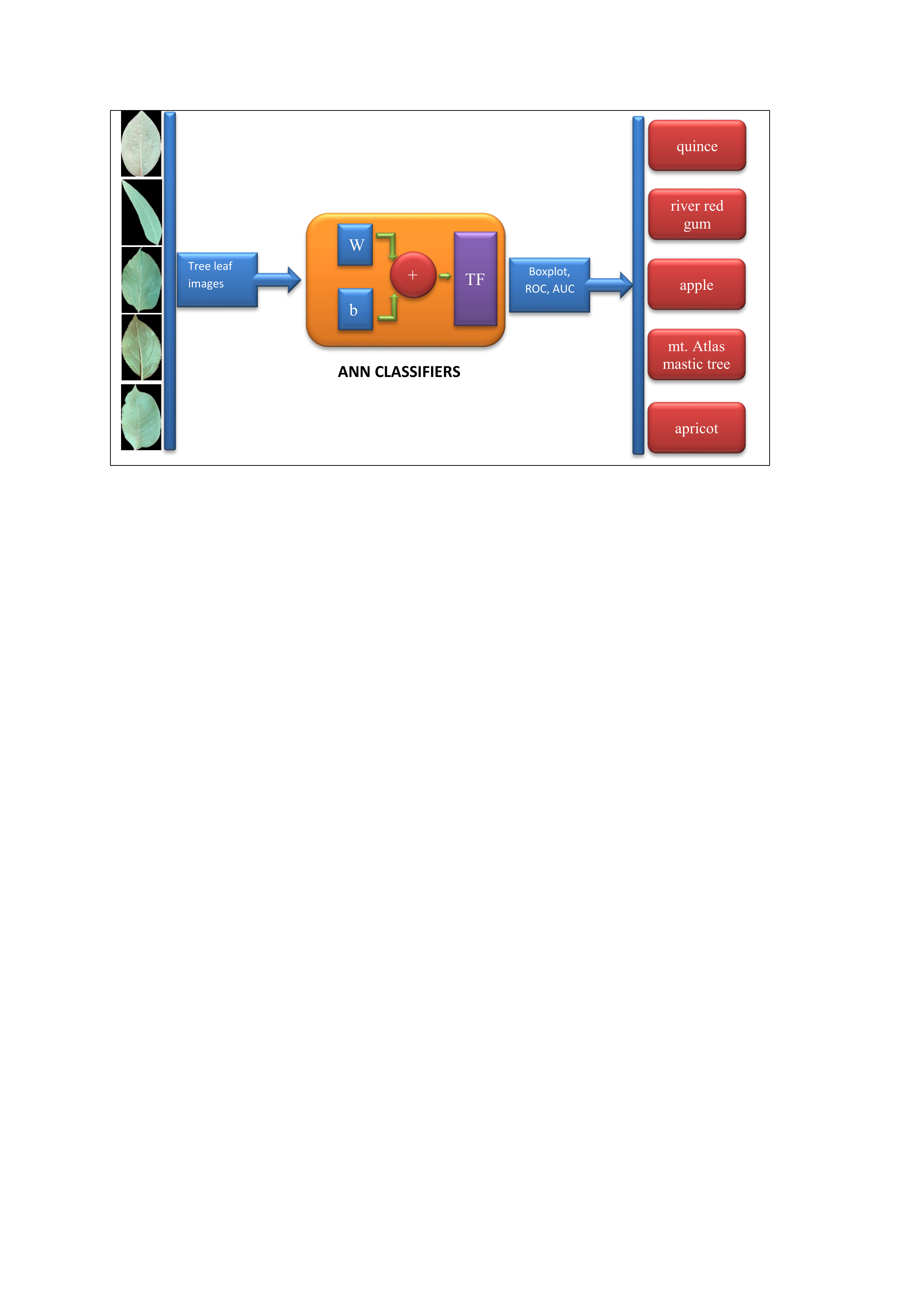
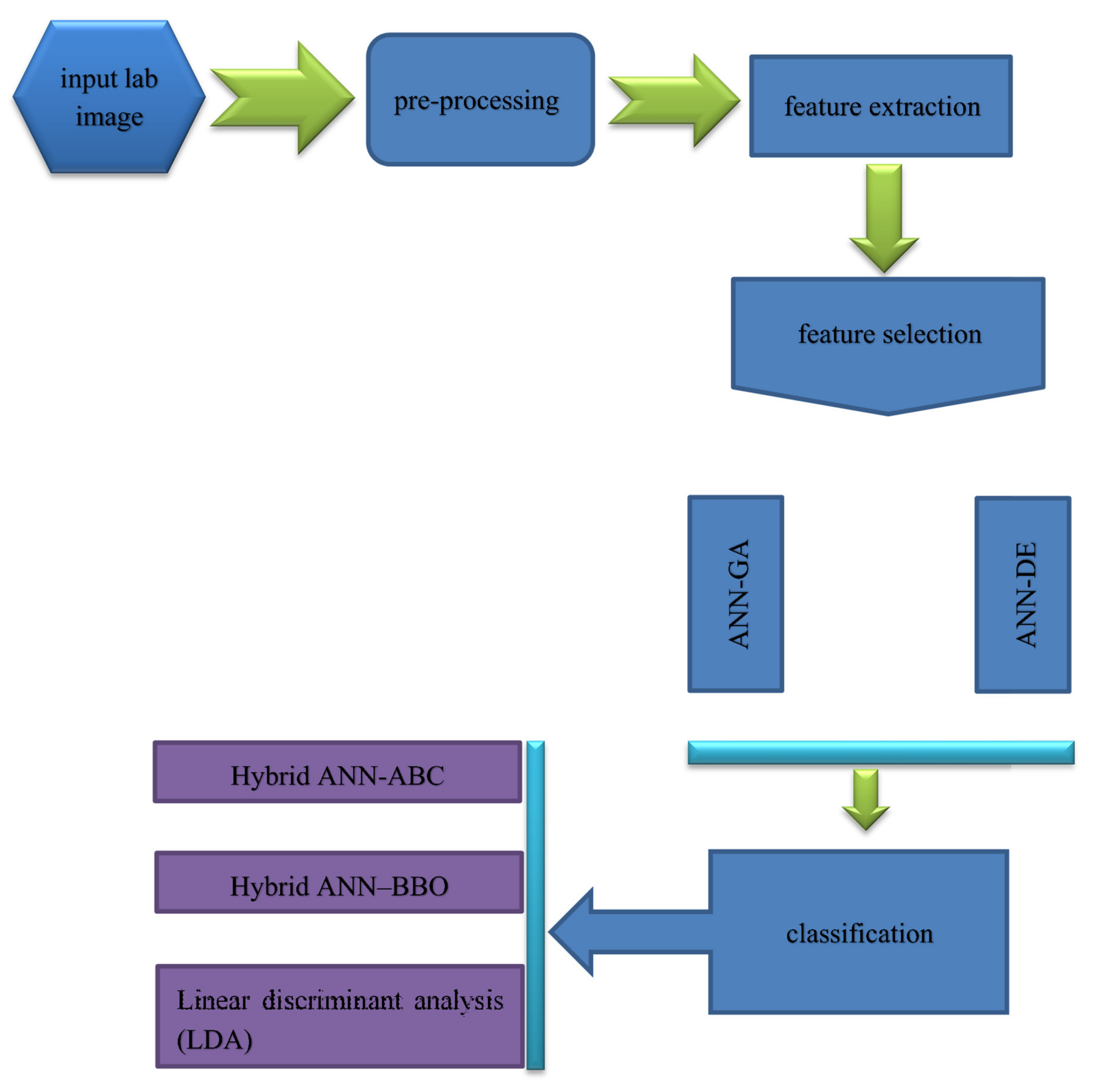
The aim of this study is to design an intelligent computer vision system to classify five species tree leaves, including 1–Cydonia oblonga (quince), 2–Eucalyptus camaldulensis dehn (river red gum), 3–Malus pumila (apple), 4–Pistacia atlantica (mt. Atlas mastic tree) and 5–Prunus armeniaca (apricot). Figure 1 depicts a flowchart of the computer vision system for plant tree leaves automatic classification, here proposed.
2. Materials and Methods
As it can be seen from Figure 1, the proposed computer vision system consists of five steps: the first step includes imaging, the second step includes segmentation and pre-processing, the third step includes feature extraction (including texture descriptors based on the histogram, texture features based on the gray level co-occurrence matrix, shape features, moment invariants, and color features), fourth step includes discriminant feature selection (based on two methods: hybrid artificial neural network–differential evolution (ANN–DE) and hybrid artificial neural network–genetic algorithm (ANN–GA)), and fifth step comprises classification based on three different classifiers, including hybrid artificial neural network–ant bee colony (ANN–ABC), hybrid artificial neural network–biogeography based optimization (ANN–BBO) and Fisher’s linear discriminant analysis (LDA). Each of the five steps in the here proposed computer vision system, depicted in Figure 1 flowchart, will be further explained with more detail in the next paper sections.
2.1. Database Used in Computer Vision
As already mentioned, in this study five different types of leaves were investigated, including 1—Cydonia oblonga (quince), see Appendix Figures A1 and A2—Eucalyptus camaldulensis dehn (river red gum), see Appendix Figures A2 and A3—Malus pumila (apple), see Appendix Figures A3 and A4—Pistacia atlantica (mt. Atlas mastic tree), see Appendix Figures A4 and A5—Prunus armeniaca (apricot), see Appendix Figure A5. Table 1 shows the class number, English common tree name, scientific tree name and the number of samples in each class. Figure 2 shows one sample of each leaf type. All images were taken in Kermanshah, Iran (longitude: 7.03°E; latitude: 4.22°N). High-quality images were taken with a color GigE industrial camera (ImagingSource, model DFK-23GM021, 1/3 inch Aptina CMOS MT9M021 sensor, 1.2 MP 1280 × 960 spatial resolution, Germany), mounting an appropriate Computar CBC Group lens (model H0514-MP2, f = 5 mm F1.4, 1/2 inch type megapixel cameras, Japan). The camera was fixed at 10 cm above ground level, and all images were taken under white light of 327 lux lighting conditions.
2.2. Image Pre-Processing and Segmentation
The segmentation stage is an important one in image processing, since in case of wrong segmentation, either the background is considered as an object (in this study, any tree leaf) or object is considered as background. To reach a proper segmentation, six standard color spaces (RGB, HSV, HSI, YIQ, CMY, and YCbCr) were taken into account to find the best color space for segmentation purposes. Results have shown that the best color space for image segmentation was YCbCr color space and the best channels for image thresholding were luminance Y and chrominance Cr channels. Equation (1) was used to set the value of the threshold used to segment objects from their background in tree leaf images:
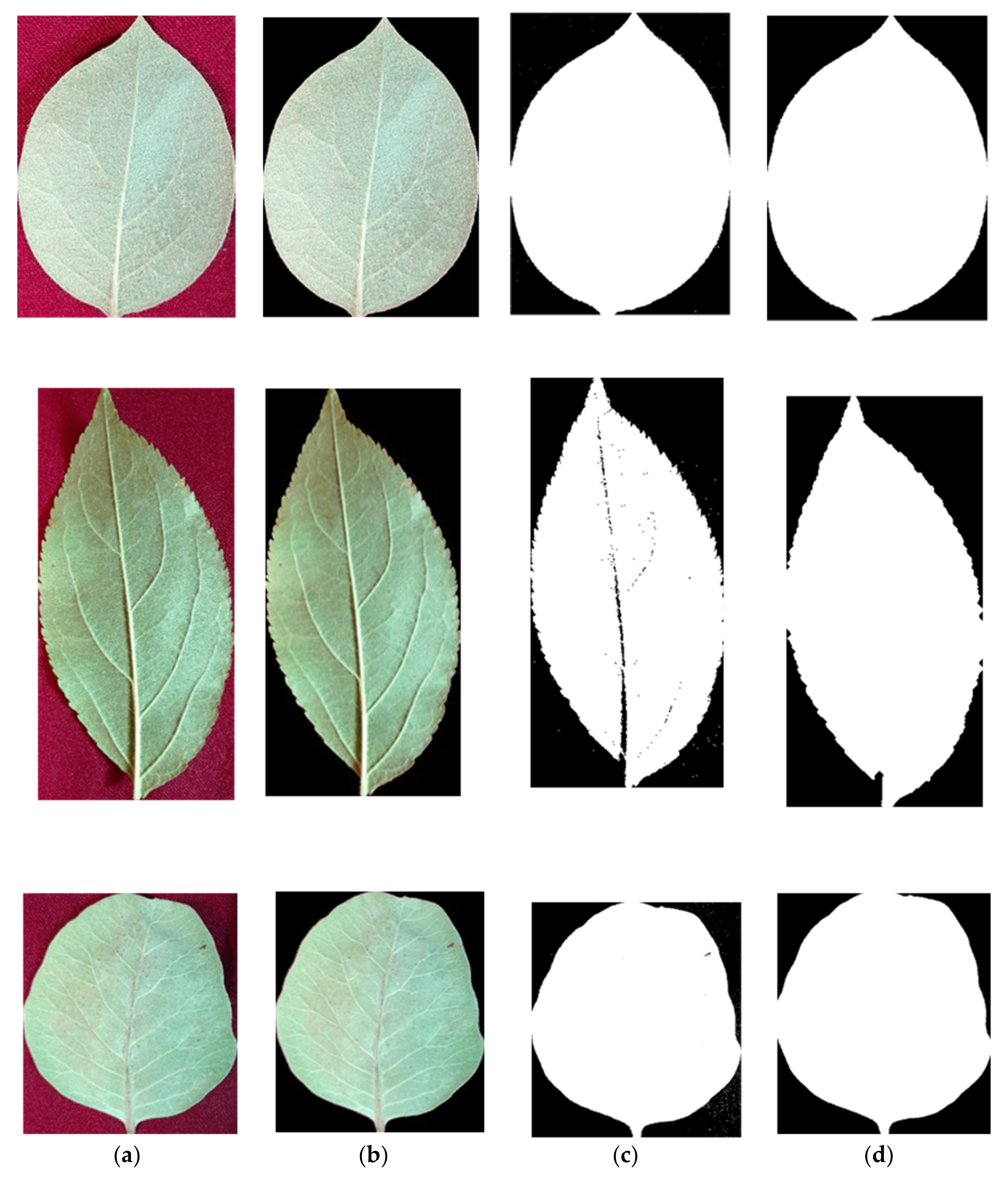
The implications of this equation are as follows: each pixel in YCbCr color space that has Y components smaller or equal to 100, or Cr components larger or equal to 15, is considered as background, otherwise, a pixel is considered as foreground (tree leaf object). In order to extract shape features from segmented images, binary images are needed. To extract shape features with high accuracy, some morphological operations are needed, since usually, some “noisy” pixels can exist in segmented images. For this reason, the Matlab imclose function was used, (Gonzalez et al. [10]). Figure 3 summarizes pre-processing operations, shown over three sample tree leaf images.
2.3. Feature Extraction
It is well-known that in order to properly classify different tree leaf types, feature extraction is needed. Features of various types and in different fields include texture descriptors based on the histogram, texture features based on the gray level co-occurrence matrix, shape features, moment invariants and color features (others may exist that are not used here). Above mentioned feature types were extracted from each leave. Indeed, the first 285 features of each leaf image were extracted and then effective (high discriminant) features were selected among them by hybrid ANN–DE and hybrid ANN–GA optimization approaches.
2.3.1. Texture Descriptors Based on the Histogram
Texture features that were extracted based on histogram include homogeneity, entropy, smoothness, third moment, average and standard deviation.
2.3.2. Texture Features Based on the Gray Level Co-Occurrence Matrix (GLCM)
It is well-known that neighbor angles have a big impact on the estimation of the values of each feature based on the GLCM. Table 2 shows texture features extracted based on the gray level co-occurrence matrix. These features were extracted for four different angles: 0°, 45°, 90°, and 135°. Thus, in total, 27 × 4 = 108 texture features were extracted from each object.
2.3.3. Shape Features
In this study, 29 shape features were extracted. Table 3 lists the shape features that were used here.
2.3.4. Moment Invariant Features
Moment invariant features have the advantage that are insensitive to translation, reflection dilation, and rotation. In this study, 10 moment-invariant features were extracted: first-order moment invariant, second-order moment invariant, third-order moment invariant, fourth-order moment invariant, fifth-order moment invariant, sixth-order moment invariant, seventh order moment invariant, difference of first and seventh order moment invariants, difference of second and sixth-order moment invariants and difference of third and fifth-order moment invariants.
2.3.5. Color Features
Different color features have different values in different color spaces. For this reason, some color features were extracted in RGB, YCbCr, YIQ, CMY, HSV and HSI color spaces. Extracted color features are divided into two groups:
- ‘Statistical’ color features
- Vegetation index color features.
‘Statistical’ Color Features
These features comprised mean and standard deviations of the first color component, the second component, third component and mean of first, second and third components for all RGB, YCbCr, YIQ, CMY, HSV, and HSI color spaces. Thus, the total number of ‘statistical’ color features was .
Vegetation Index Color Features
Table 4 lists 14 vegetation index features for RGB color space, including mathematical definitions. These features were also computed for the other five color spaces (YCbCr, YIQ, CMY, HSV, and HSI) totaling vegetation index features.
2.4. Discriminant Feature Selection
As mentioned before, 285 features were extracted from each leaf image object. The use of all features as input to classifiers is not wise, given the problem of overfitting and poor generalization to the test set. The selection of discriminant groups of features is a well-known good practice. To do so, two methods based on artificial intelligence were used to select effective features (results to be shown later on):
- ANN–DE
- ANN–GA.
2.5. Optimal Neural Network Classifier Parameters
Classification is the final step in designing a computer or machine vision system. A high-performance classifier guarantees the accuracy of the computer version system. In this study, three classifiers including hybrid ANN–ABC, hybrid ANN–BBO and Fisher’s linear discriminant analysis (LDA), were used in classifying. In order to have statistically valid results, 100 uniform random simulations were repeated. All data were divided into two disjoint groups, training, and validation set data (60% input samples) and test set data (40% of input samples) in each of the 100 averaged simulations, following a uniform random distribution with probability 0.6 and 0.4 to belong to train/validation and test sets, respectively. It is worth mention that a multilayer perceptron (MLP) ANN was used. An MLP neural network has five adjustable parameters: number of neural network layers, number of neurons in each layer, nonlinear transfer function, back-propagation network training function, and back-propagation weight/bias learning function. ABC and BBO algorithms were used to select optimal MLP parameter values. Table 5 shows the optimum values of the MLP parameters which were determined with ABC and BBO algorithms.
3. Results and Discussion
To evaluate the three different classifiers’ performance (hybrid ANN-ABC, hybrid ANN–BBO and LDA), various criteria are computed, including confusion matrix, sensitivity, specificity and accuracy, receiver operating characteristic (ROC) and area under the ROC curve (AUC). Before the evaluation of the classifiers’ performance, selected features based on ANN–DE and ANN–GA approaches are shown next.
3.1. Feature Selection Based on ANN–DE and ANN–GA Approaches
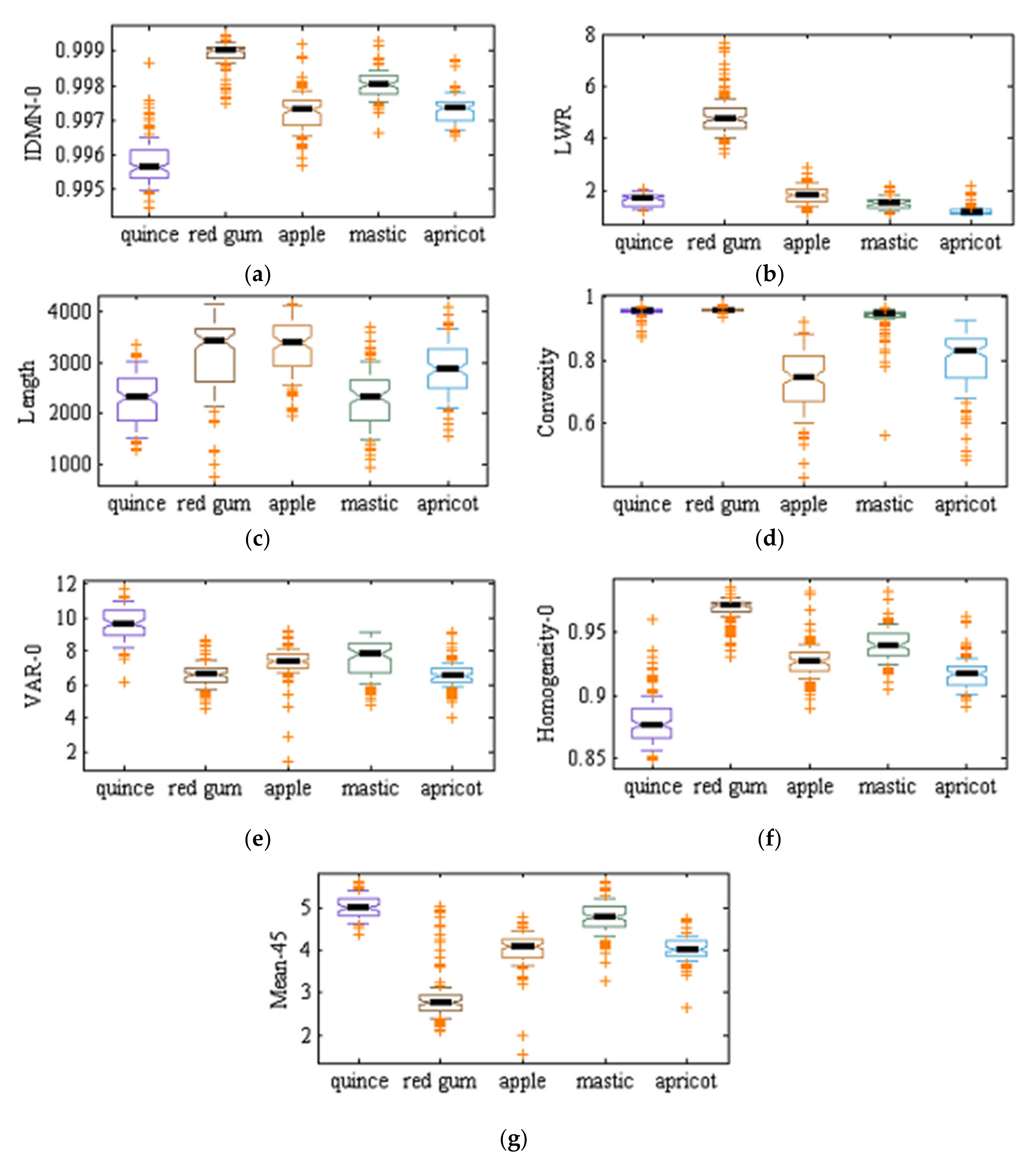
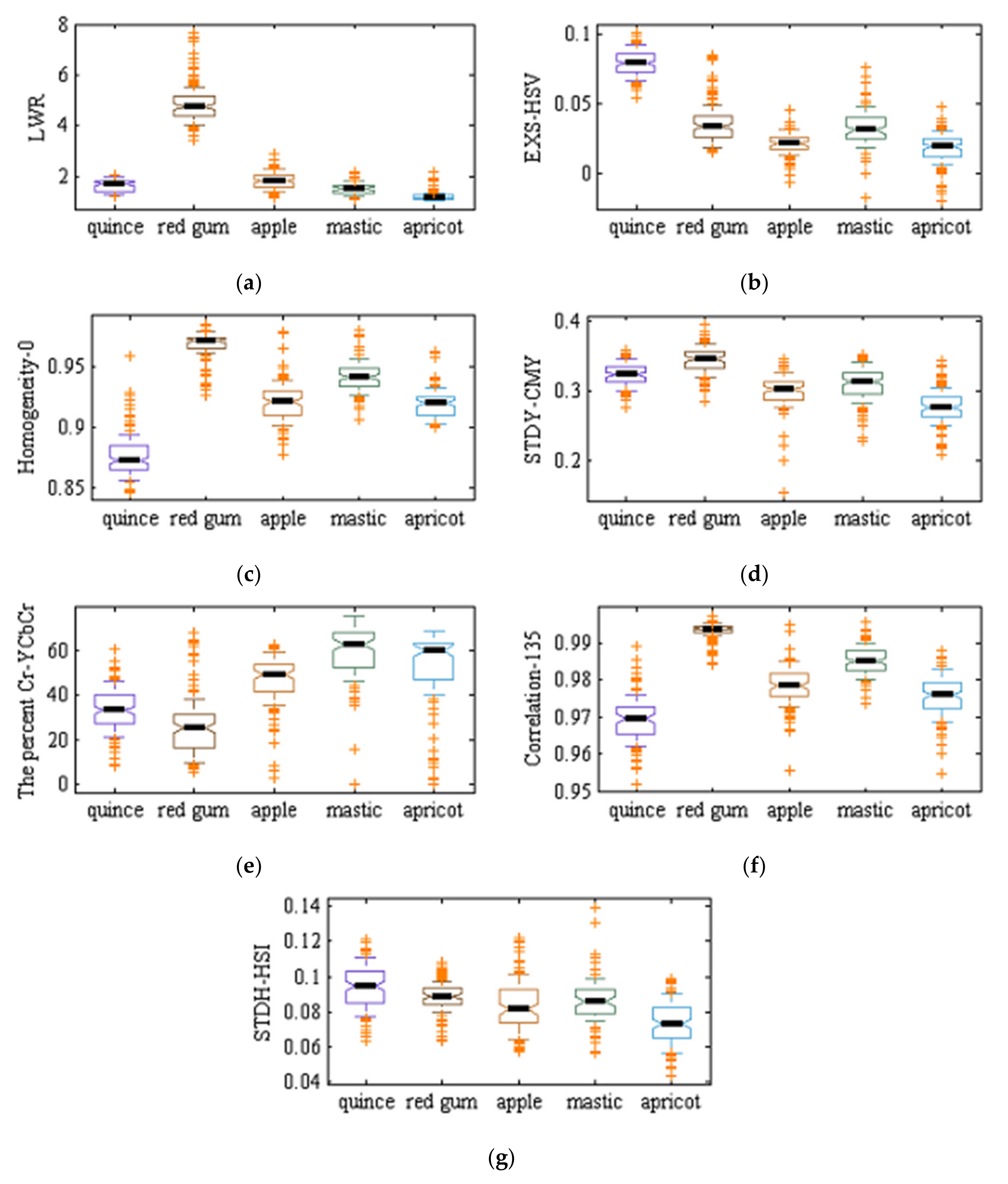
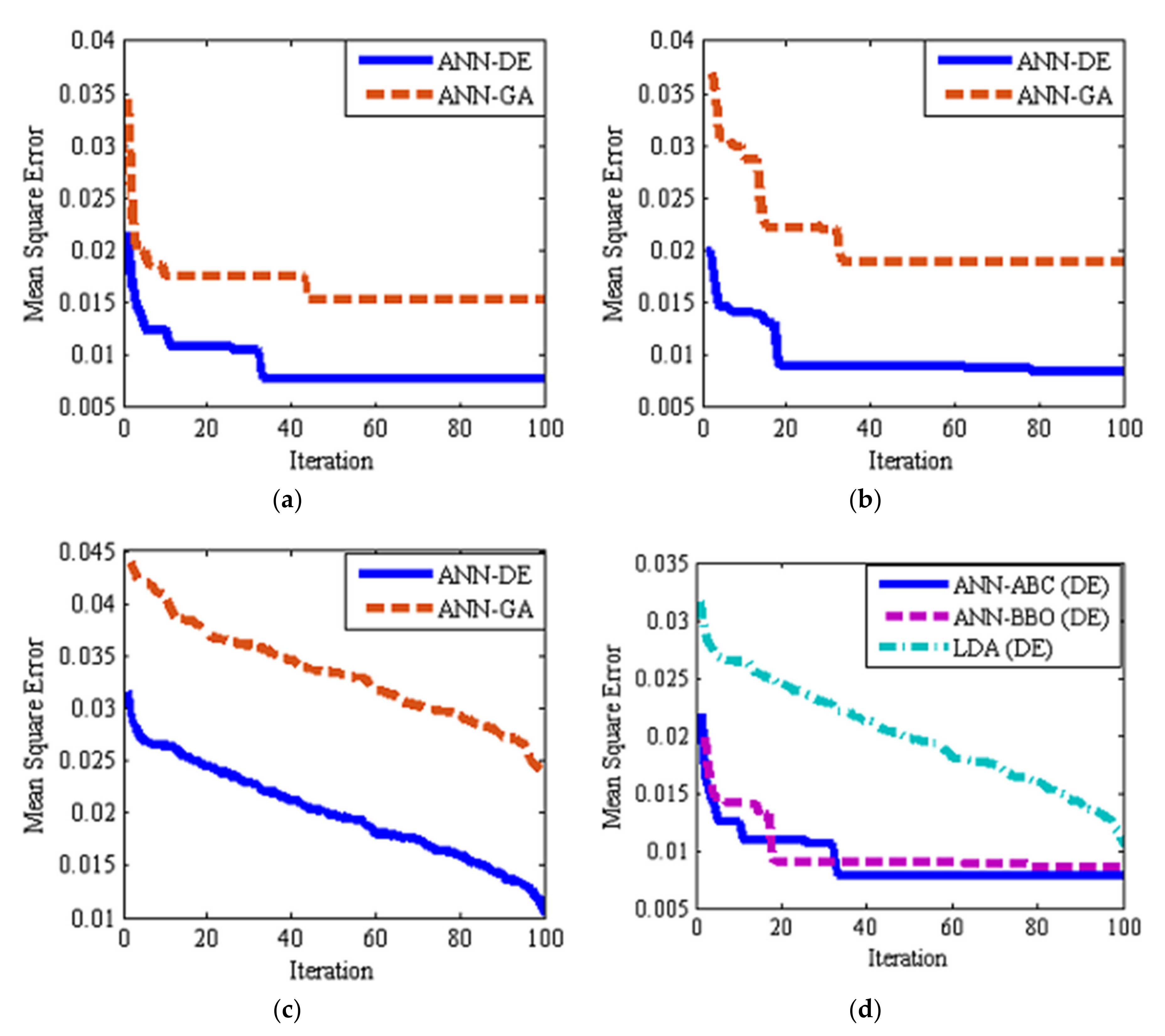
As mentioned in previous sections, two ANN–DE and ANN–GA approaches were used to select effective (discriminant) features. Table 6 shows the seven selected features by ANN–DE and ANN–GA. As one can see, ANN–DE method selected all features among shape and texture features based on the gray level co-occurrence matrix, while the ANN–GA method selects discriminant features among shape, texture based on the gray level co-occurrence matrix and color features. Figure 4 and Figure 5 show boxplot graphs for the value of each extracted feature by ANN–DE and ANN–GA methods, respectively. Figure 4 (ANN–DE) shows that quince, red gum, mastic tree, and apricot classes can be separated based on only three features, inverse difference moment normalized related to 0 degrees (IDMN_0), homogeneity related to 0 degree (homogeneity_0) and mean related to 45 degrees (mean_45), since those features have the lowest overlapping boxplots among classes. The same can be said, for obvious reasons, about Figure 5c (ANN–GA) regarding homogeneity related to 0 degrees (homogeneity_0) feature. Figure 6 shows the validation step, where we plot mean square error (MSE) as a function of iteration number while learning for hybrid ANN–ABC, hybrid ANN–BBO and LDA classifiers, based on the selected features obtained with ANN–DE and ANN–GA methods listed above. Figure 6a–c show that MSE for selected features based on ANN–DE are lower than those MSE for selected features based on ANN–GA. Having said that, selected features by ANN–DE were finally used as input in getting the classification results.
3.2. Classification Based on Hybrid ANN–ABC, Hybrid ANN–BBO and LDA
In this study, three classifiers were used: hybrid ANN–ABC, hybrid ANN–BBO and LDA. To achieve statistical valid results, we averaged 100 simulations with uniform random train and test sets; the probability of an input sample to belong to the train set was 0.6 and 0.4 to belong to the test set.
3.2.1. Classification Based on the Hybrid ANN–ABC
Table 7 shows confusion matrix classification results, using ANN–ABC classifier for 100 iterations, over the test set. The lowest classifier error value is that of red gum class with only 17 misclassified samples among 4703 total test samples, resulting in accuracy above 99.6% for this class. The highest classifier error value is given in the mastic tree class, where 453 out of 3542 samples were misclassified, resulting in a misclassification rate of 12.79%. Figure 2 shows that the shape of 2–Eucalyptus camaldulensis dehn samples (river red gum) are very different from other class samples, so samples related to this class are classified with high accuracy. On the other hand, as a possible explanation to previous facts, Figure 2 shows how river red gum tree leaves are quite different in shape to other four tree leaves species, which at the same time have quite similar shapes among them, thus resulting in most misclassification errors among these four classes. In summary, the ANN–ABC classifier classified the 20,700 test samples with an accuracy above 94%, which has to be judged as very good for our tree leaf image database.
3.2.2. Classification Based on the Hybrid ANN–BBO
Table 8 shows confusion matrix classification results using hybrid ANN–BBO classifier for 100 iterations averaged, over the test set. As can be seen, 2230 samples from 20,700 samples were misclassified by this classifier (10.77%). Again, the lowest ANN–BBO classifier accuracy is for mastic tree (82.20%) and the highest classifier accuracy is again for river red gum tree (94.60%), similar to the hybrid ANN–ABC classifier, and considered as promising results, despite on average the ANN–BBO classifier performance is behind its partners.
3.2.3. Classification Based on LDA
Table 9 shows classification results presented as a confusion matrix for the LDA classifier for 100 uniform random train and test set iterations averaged, over the test set. The interesting thing here is that the LDA classifier classified all samples in the river red gum class correctly. So it can be concluded that for easy class data, the LDA classifier has higher accuracy. On the other hand, the LDA classifier has less accuracy than the hybrid ANN–ABC classifier in quince and apricot classes. Finally, one can see how LDA classifier classified all test data with an overall accuracy of 93.99%, that is high accuracy very close to the 94.04% overall accuracy for the ANN–ABC classifier, and both clearly over the 89.23% overall accuracy for the ANN–BBO classifier, which performed the poorest of the three.
3.3. Classifiers Performance: Evaluation
Two common methods to evaluate classifiers performance over the test set are:
- Based on the sensitivity, specificity, and accuracy values (confusion matrix).
- Based on receiver operating characteristic (ROC) and area under the ROC curve (AUC).
We evaluate classifiers using both methods next.
3.3.1. Classification Performance Based on the Sensitivity, Specificity, and Accuracy Values (Confusion Matrix)
With sensitivity, specificity and accuracy criteria, one can evaluate a classifier system based on correct and wrong classified samples, detailing between which classes errors are taken place if needed. Sensitivity, specificity, and accuracy are defined next in Equations (2)–(4):
where true-positive fraction (TP) is equal to the number of samples in each class that are correctly classified, true-negative fraction (TN) is equal to the number of samples on main diagonal in confusion matrix (square matrix that has dimensions equal to number of classes, cf. Table 7, Table 8 and Table 9) minus the number of samples that are correctly classified in the intended class, false-negative fraction (FN) is defined as the sum of horizontal samples in the investigated class minus number of samples that are correctly classified in the intended class, and false-positive fraction (FP) is defined as the sum of vertical samples of the investigated class minus the number of samples that are correctly classified in the intended class (Wisaeng [17]). In short, a sensitivity value of 100% in a certain class means that all samples of this class were classified correctly; a specificity value of 100% in a certain class means that no samples from other classes were misclassified in that given class; and an accuracy value of 100% means that neither no samples from other classes were misclassified in a certain class nor any samples from that certain class were misclassified in other classes.
Table 10 shows classification performance criteria including specificity, sensitivity and accuracy results for 100 uniform random iterations using hybrid ANN–ABC, hybrid ANN–BBO and LDA classifiers. By looking carefully at Table 10, one realizes that the LDA classifier is in general terms superior to both ANN–ABC (slightly) and ANN–BBO (clearly), that red river gum tree class is consistently easier to classify among all three classifiers, and that opposite situation happens with mt. Atlas mastic tree class. In precise terms, the following results are reached: best classifier, mean sensitivity, and mean specificity, were computed for the five trees under study, resulting in 1–Cydonia oblonga (quince) 95.89% (ANN–ABC), 95.91% (ANN–ABC); 2–Eucalyptus camaldulensis dehn (river red gum) 100% (LDA), 100% (LDA); 3–Malus pumila (apple) 96.63% (LDA), 94.99% (LDA); 4–Pistacia atlantica (mt. Atlas mastic tree), 91.71% (LDA), 82.57% (LDA); and 5–Prunus armeniaca (apricot) 88.67% (LDA), 94.65% (LDA), respectively, all over the test set.
3.3.2. Classification Performance Based on ROC and AUC
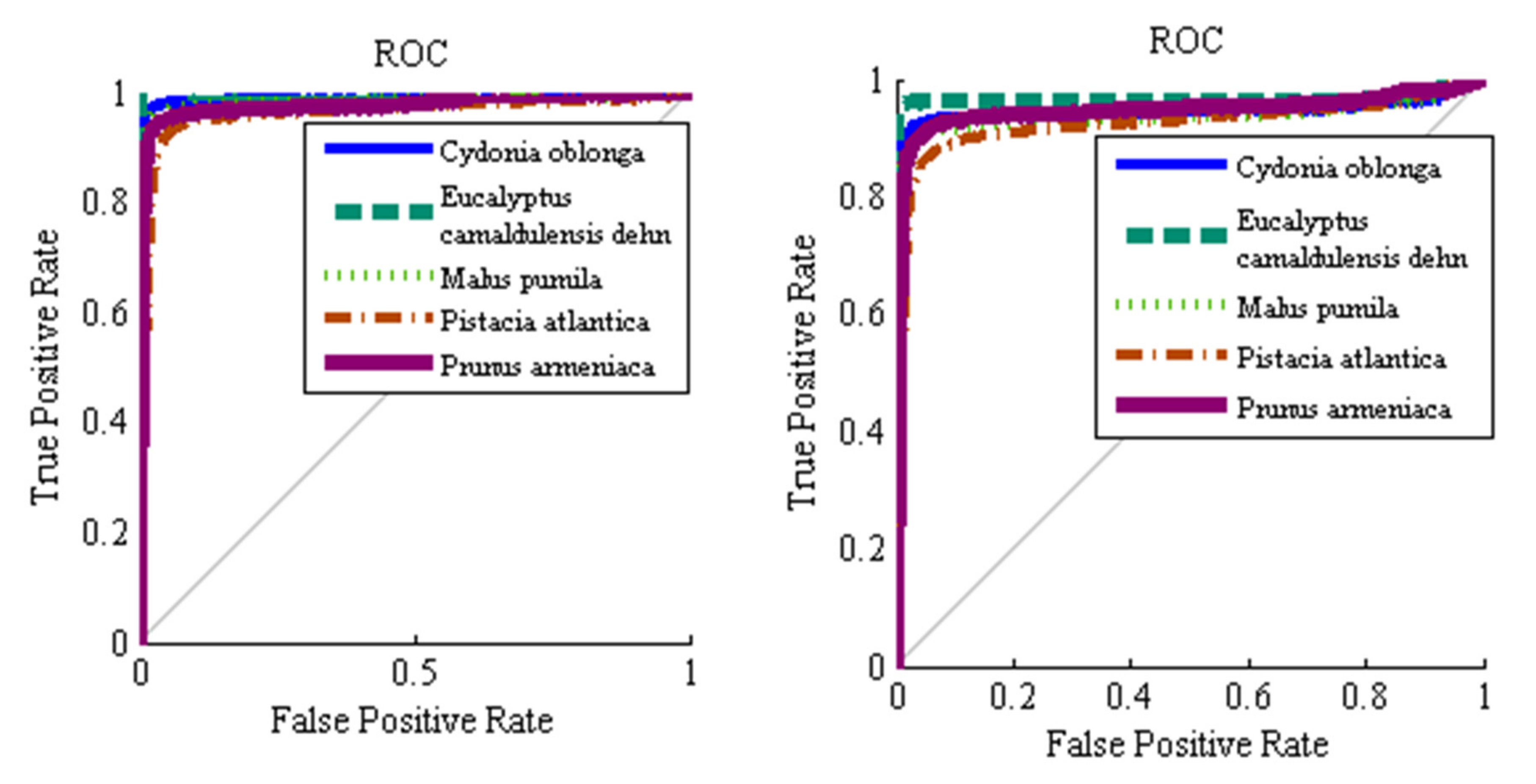
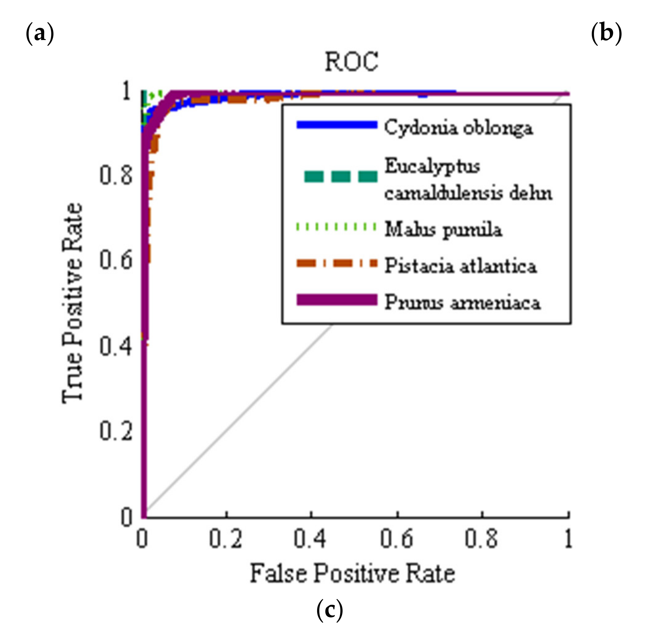
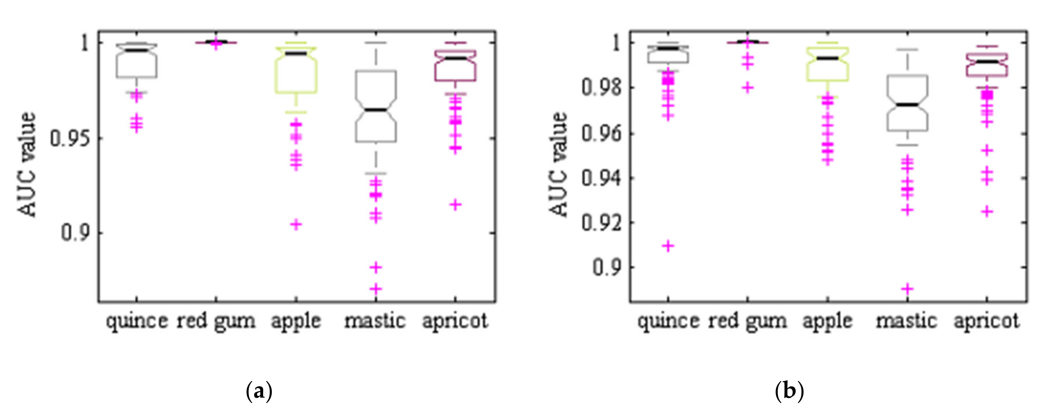
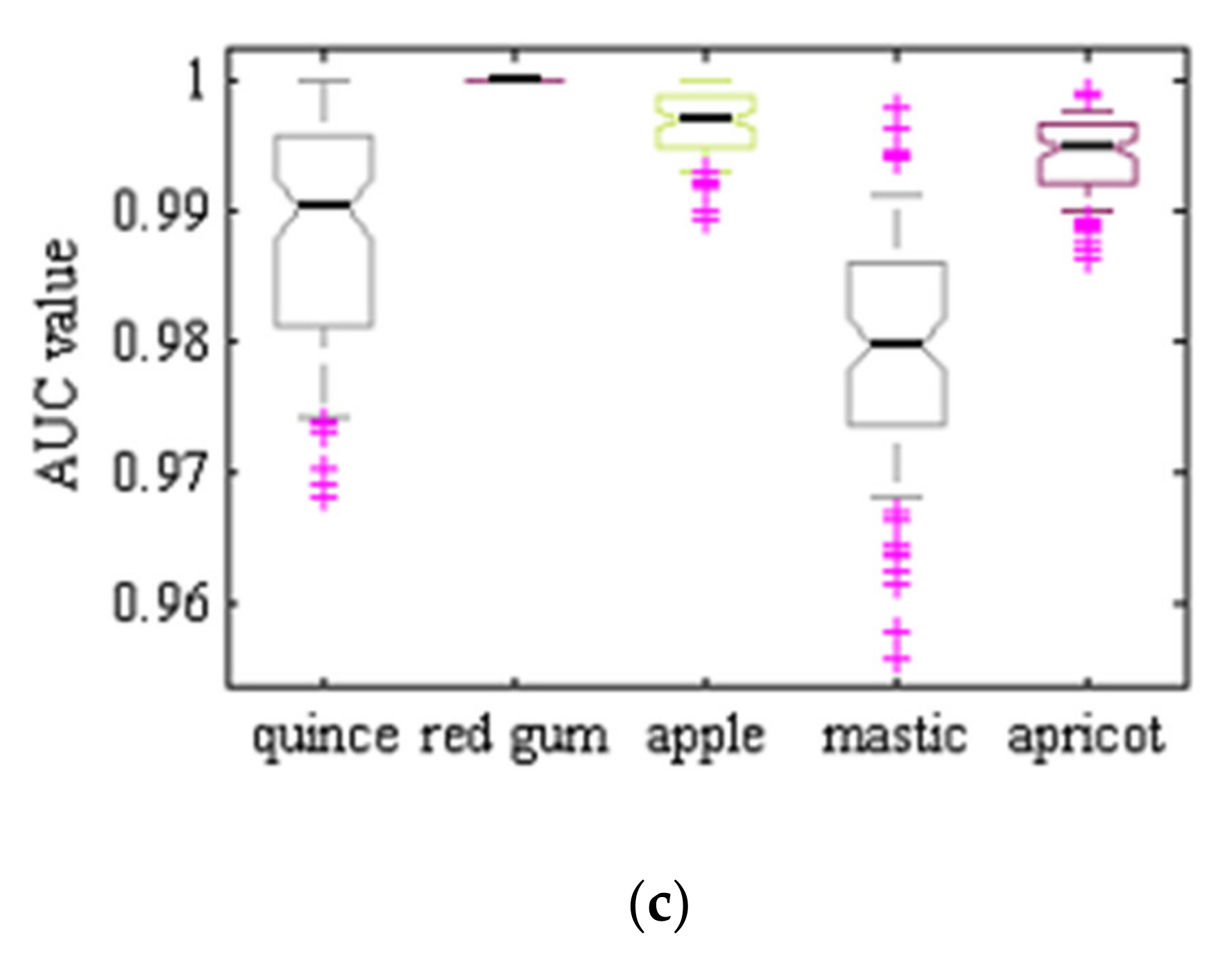
Figure 7 shows ROC graphs for the different classes and different classifiers considered. In short, when plotting ROC curves, we are plotting FPR versus TPR, on the specificity-sensitivity plane. The higher the AUC values is the higher the classifier accuracy, while having an value is totally useless and simply equivalent to a random toss of a coin. As one can see, the ROC graphs related to hybrid ANN–ABC and LDA classifiers are near the upright end, so this implies that these two classifiers have good accuracy. At the same time, in Table 11 we show the mean and standard deviation of AUC values for the five different classes and three classifiers under consideration, over 100 repeated uniform random iterations. Figure 8 shows AUC boxplot graphs for 100 iterations based on ANN–ABC, ANN–BBO and LDA classifiers. As one can see, these three classifiers classified red river gum class samples with extremely high accuracy, since boxplot graphs are very compact. Also, LDA if often ahead of its partners, closely followed by ANN–ABC, in terms of AUC values (please note that vertical axis AUC ranges are different in each figure). In precise terms, mean AUC values were computed for the five trees under study, resulting in 1–Cydonia oblonga (quince) 0.991 (ANN–ABC); 2–Eucalyptus camaldulensis dehn (river red gum) 1.00 (LDA); 3–Malus pumila (apple) 0.996 (LDA); 4–Pistacia atlantica (mt. Atlas mastic tree) 0.979 (LDA); and 5–Prunus armeniaca (apricot) 0.994 (LDA), respectively, all over the test set.
Finally, to compare the CCR in this study with others, Singh and Bhamrah [2], Kadir [3], Mursalin et al., [5] and Ehsanirad [4], were used. It should be noted that since studies do not share the same leave image database, no direct comparison is possible. Singh and Bhamrah [2] classified 8 species of different plants with artificial neural network classifier and Kadir [3] used a Bayes classifier to classify some leaves related to several plants. Mursalin et al., [5] used some shape and color features for plant classification purposes. Ehsanirad [4] used only some texture features for the classification of different plants. Table 12 shows the accuracy or CCR of the different classification methods for comparison purposes. As one can see, the proposed method has a higher number of samples and higher accuracy than the other methods being compared with.
One possible reason for the superiority of the proposed method might be the use of different properties. As can be seen in Section 2.3, feature extraction, in this study several features comprising five different feature types were extracted. That can be of help in finding effective discriminative features that can properly separate different plant type leaves. While on the contrary, other researchers often used only a couple of feature types, such as color and texture features. A second possible reason for higher accuracy might refer to the structure of the neural network since the study here proposed the optimal structure of the ANN is adjusted by both ABC and BBO algorithms.
4. Conclusions
This study aims to design an imaging computer vision system to classify five types of tree leaf images. Relevant results can be summarized as follows to conclude:
- Tree leaves images had the lowest level of noise (noise pixels) after segmentation in YCbCr color space, in comparison with RGB, YIQ, CMY, HSV and HSI color spaces.
- Two channels in YCbCr color space were needed to image thresholding (a luminance and a chrominance channels).
- Among the seven discriminant features selected, four features were texture features based on the gray level co-occurrence matrix and three features were shape features.
- We believe that since samples in 2–Eucalyptus camaldulensis dehn (river red gum, class 2) have clear different shapes, shape features were selected as effective features, reaching almost no classification errors inside 2–Eucalyptus camaldulensis dehn (river red gum) class.
- Whenever features in different classes do not present overlapping, the statistical LDA method usually has a superior performance.
Author Contributions
Conceptualization, S.S. R.P. and J.I.A.; methodology, S.S. and J.I.A.; software, S.S.; validation, S.S. and J.I.A.; formal analysis, S.S. and J.I.A.; investigation, S.S. and J.I.A.; resources, S.S.; data curation, J.I.A.; writing—original draft preparation, J.I.A.; writing—review and editing, S.S., R.P. and J.I.A.; visualization, S.S. and R.P.; supervision, J.I.A.; project administration, J.I.A. All authors have read and agreed to the published version of the manuscript.
Funding
This research was funded in part by the European Union (EU) under the Erasmus+ project entitled “Fostering Internationalization in Agricultural Engineering in Iran and Russia” [FARmER] with grant number 585596-EPP-1-2017-1-DE-EPPKA2-CBHE-JP.
Conflicts of Interest
The authors declare no conflict of interests.
Appendix A
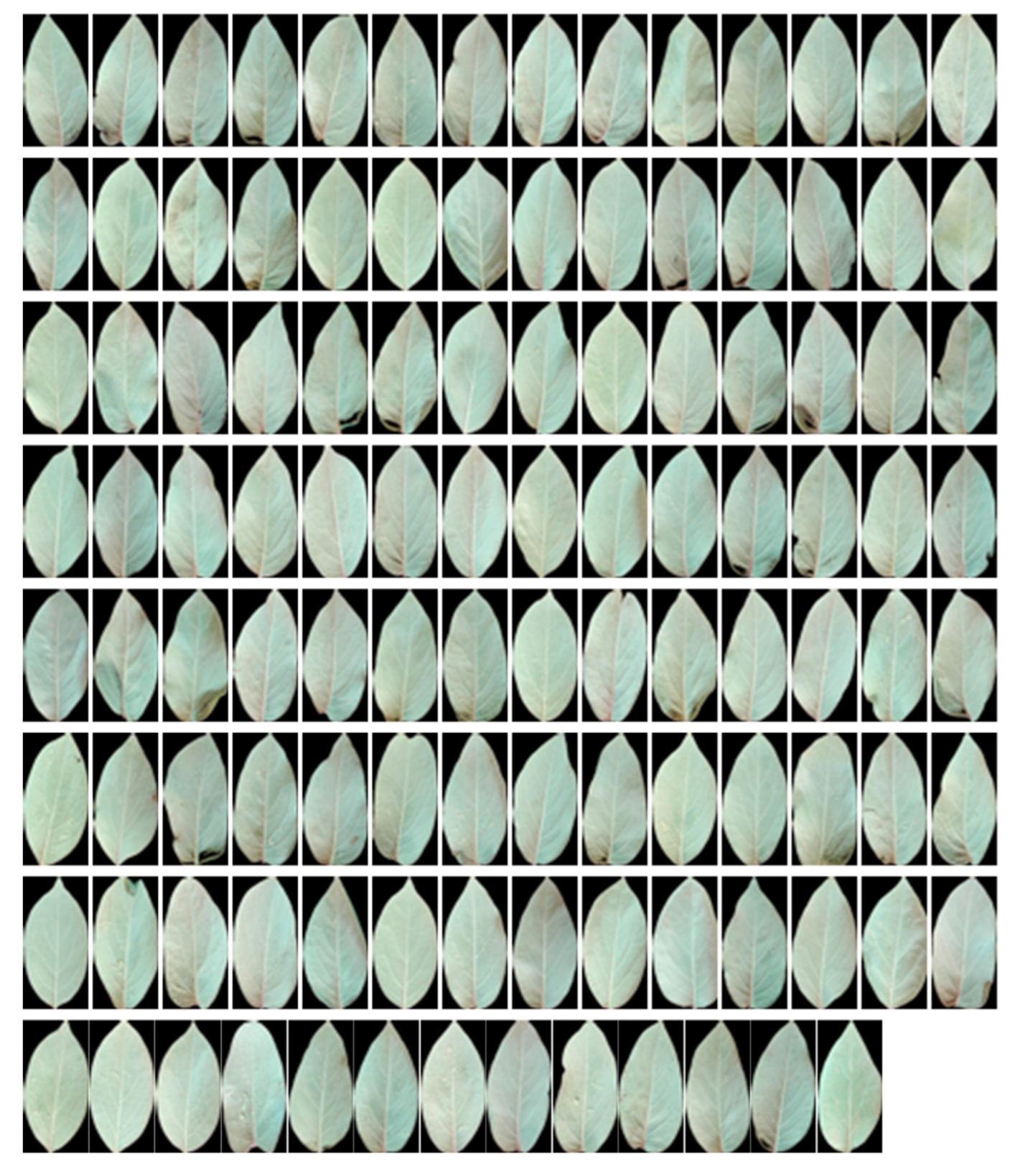
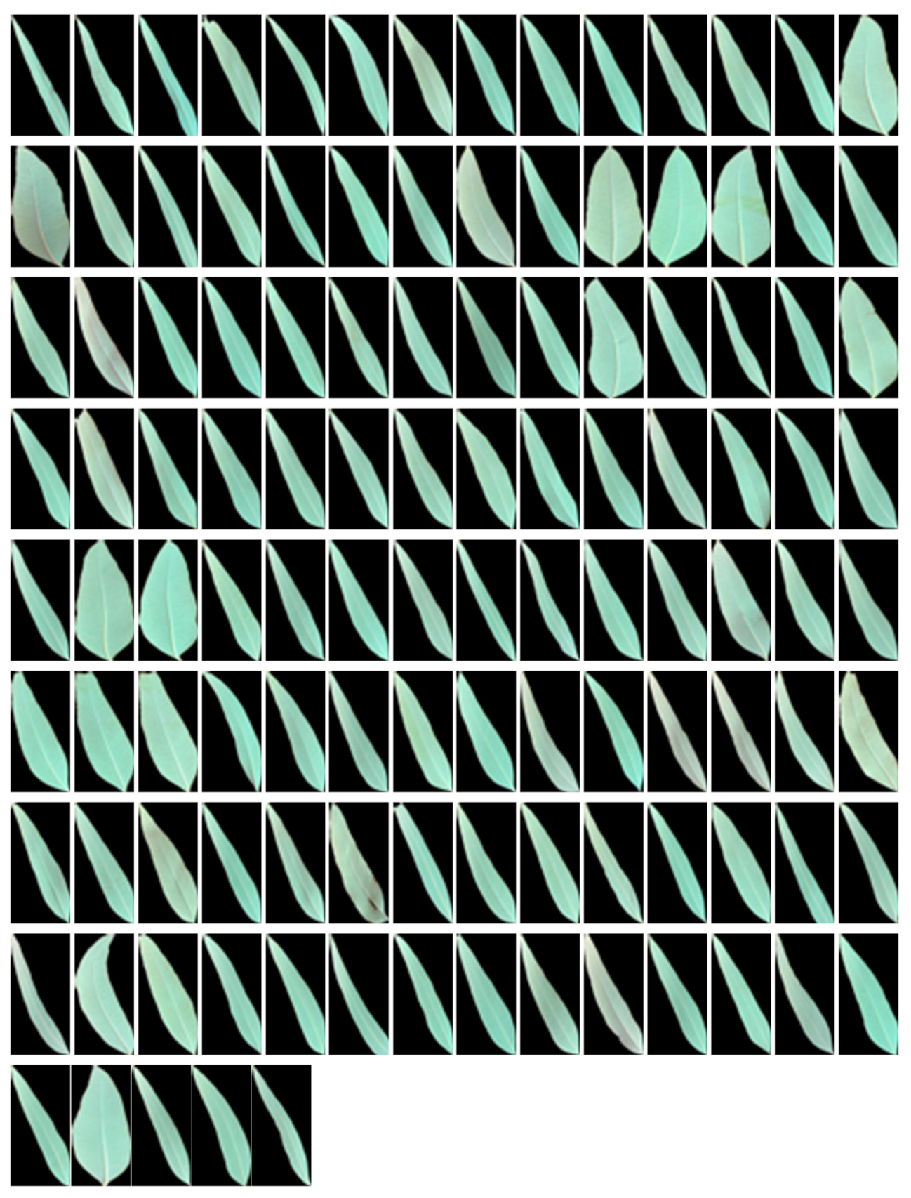
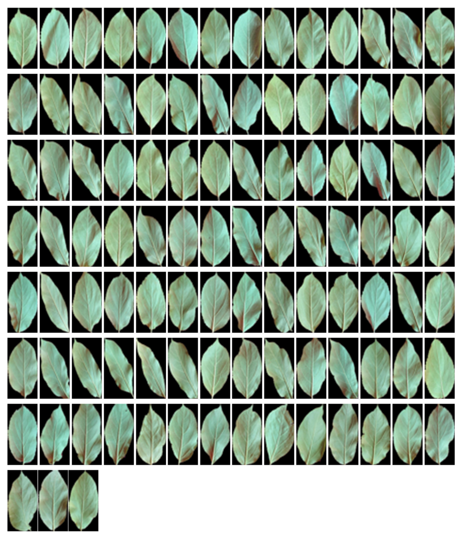
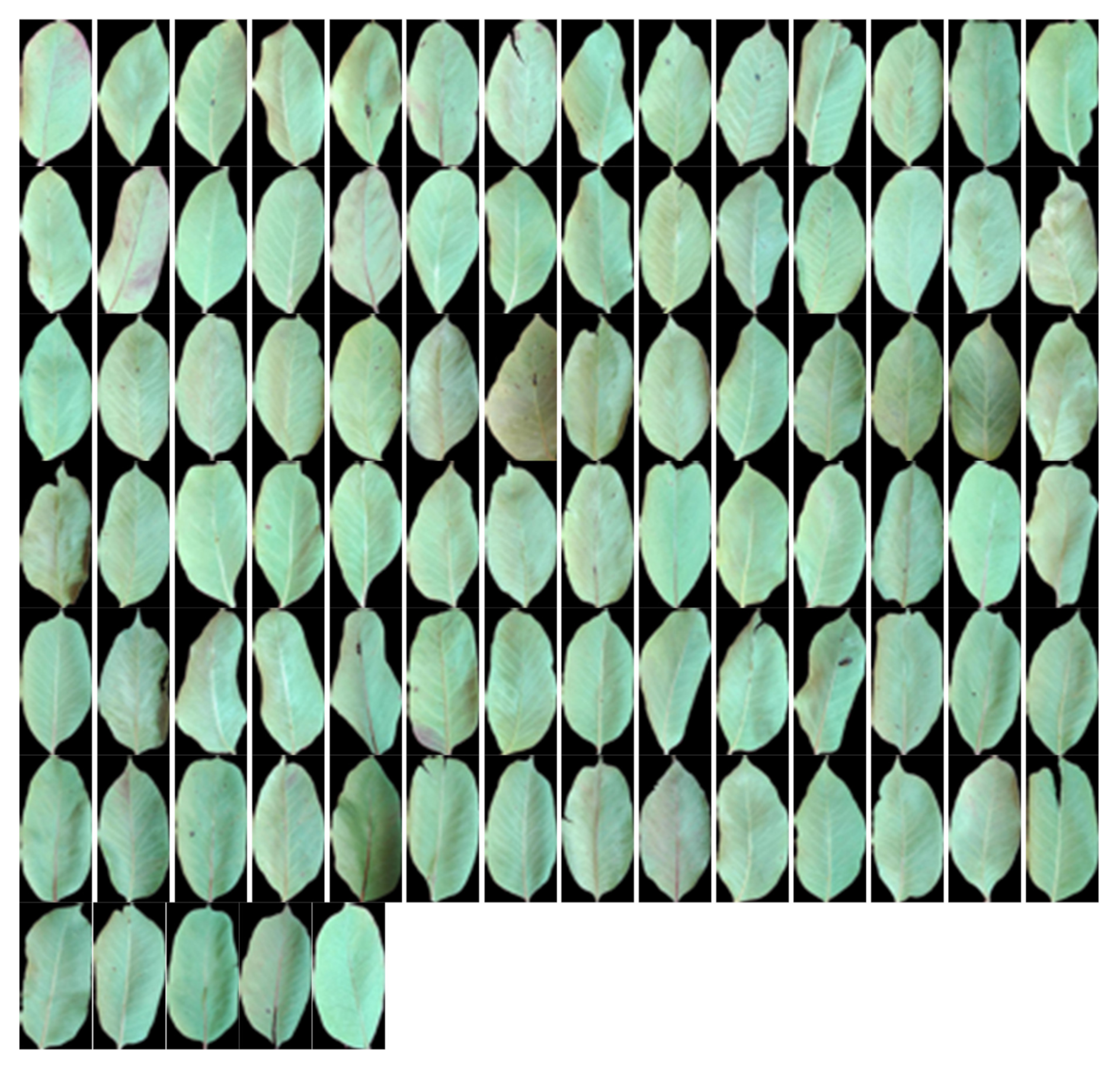
We depict next all five type 516 segmented tree leaves image database, as shown in Figure A1, Figure A2, Figure A3, Figure A4 and Figure A5, corresponding to, 1—Cydonia oblonga (quince), 2—Eucalyptus camaldulensis dehn (river red gum), 3—Malus pumila (apple), 4—Pistacia atlantica (mt. Atlas mastic tree) and 5—Prunus armeniaca (apricot), respectively.
Figure A1.
Cydonia oblonga (quince) tree leaves image database: 111 samples.

Figure A2.
Eucalyptus camaldulensis dehn (river red gum) tree leaves image database: 117 samples.

Figure A3.
Malus pumila (apple) tree leaves image database: 101 samples.

Figure A4.
Pistacia atlantica (mt. Atlas mastic tree) tree leaves image database: 89 samples.

Figure A5.
Prunus armeniaca (apricot) tree leaves image database: 98 samples.

References
- Liu, F.H.; O’Connell, N.V. Off-site movement of surface-applied simazine from a citrus orchard as affected by irrigation incorporation. Weed Sci. 2002, 50, 672–676. [Google Scholar] [CrossRef]
- Singh, S.; Bhamrah, M.S. Leaf identification using feature extraction and neural network. IOSR J. Electron. Commun. Eng. 2015, 10, 134–140. [Google Scholar]
- Kadir, A. Leaf Identification Using Fourier Descriptors and Other Shape Features. Gate Comput. Vis. Pattern Recognit. 2015, 1, 3–7. [Google Scholar] [CrossRef]
- Ehsanirad, A. Plant classification based on leaf recognition. Int. J. Comput. Sci. Inform. Sec. 2010, 8, 78–81. [Google Scholar]
- Mursalin, M.; Hossain, M.; Noman, K.; Azam, S. Performance Analysis among Different Classifier Including Naive Bayes, Support Vector Machine and C4.5 for Automatic Weeds Classification. Glob. J. Comput. Sci. Technol. Graph. Vis. 2013, 13, 11–16. [Google Scholar]
- Ahmed, F.; Al-Mamun, H.A.; Bari, A.S.M.H.; Hossain, E.; Kwan, P. Classification of crops and weeds from digital images: A support vector machine approach. Crop Prot. 2012, 40, 98–104. [Google Scholar] [CrossRef]
- Rumpf, T.; Römer, C.; Weis, M.; Sökefeld, M.; Gerhards, R.; Plümer, L. Sequential support vector machine classification for small-grain weed species discrimination with special regard to Cirsium arvense and Galium aparine. Comput. Electron. Agric. 2012, 80, 89–96. [Google Scholar] [CrossRef]
- Pereira, L.A.M.; Nakamura, R.Y.M.; Souza, G.F.S.d.; Martins, D.; Papa, J.P. Aquatic weed automatic classification using machine learning techniques. Comput. Electron. Agric. 2012, 87, 56–63. [Google Scholar] [CrossRef]
- Azlah, M.A.F.; Chua, L.S.; Rahmad, F.R.; Abdullah, F.I.; Wan Alwi, S.R. Review on Techniques for Plant Leaf Classification and Recognition. Computers 2019, 8, 77. [Google Scholar] [CrossRef] [Green Version]
- Gonzalez, R.C.; Woods, R.E.; Eddins, S.L. Digital Image Processing Using MATLAB; Prentice Hall: Upper Saddle River, NY, USA, 2004. [Google Scholar]
- Woebbecke, D.; Meyer, G.E.; Bargen, K.V.; Mortensen, D.A. Color indices for weed identification under various soil, residue, and lighting conditions. Trans. ASAE 1995, 3, 259–269. [Google Scholar] [CrossRef]
- Meyer, G.E.; Mehta, T.; Kocher, M.F.; Mortensen, D.A.; Samal, A. Textural imaging and discriminant analysis for distinguishing weeds for spot spraying. Trans. ASAE 1998, 41, 1189–1197. [Google Scholar] [CrossRef]
- Kataoka, T.; Kaneko, T.; Okamoto, H.; Hata, S. Crop growth estimation system using machine vision. In Proceedings of the IEEE/ASME International Conference Advances Intelligence Mechatronics (AIM 2003), Kobe, Japan, 20 July–24 July 24 2003; pp. 1079–1083. [Google Scholar]
- Meyer, G.E.; Neto, J.A.C. Verification of color vegetation indices for automated crop imaging applications. Comput. Electron. Agric. 2008, 63, 282–293. [Google Scholar] [CrossRef]
- Woebbecke, D.M.; Meyer, G.E.; Bargen, K.V.; Mortensen, D.A. Plant species identification, size, and enumeration using machine vision techniques on near-binary images. Opt. Agric. For. 1992, 1836, 208–219. [Google Scholar]
- Golzarian, M.R.; Frick, R.A. Classification of images of wheat, ryegrass and brome grass species at early growth stages using principal component analysis. Plant Meth. 2011, 7, 7–28. [Google Scholar] [CrossRef] [PubMed] [Green Version]
- Wisaeng, K. A Comparison of Decision Tree Algorithms For UCI Repository Classification. Int. J. Eng. Trends Technol. 2013, 4, 3393–3397. [Google Scholar]
Figure 1.
Flowchart of the proposed computer vision system applied in tree leaves automatic classification.
Figure 1.
Flowchart of the proposed computer vision system applied in tree leaves automatic classification.

Figure 2.
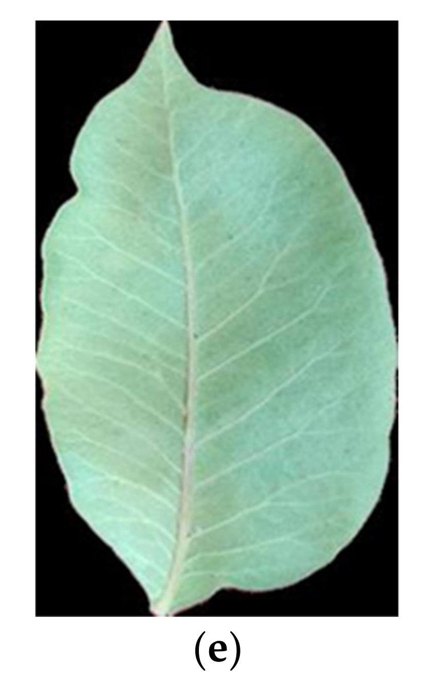
An image sample of each tree leaf type: (a) 1–Cydonia oblonga (quince), (b) 2–Eucalyptus camaldulensis dehn (river red gum), (c) 3–Malus pumila (apple), (d) 4–Pistacia atlantica (mt. Atlas mastic tree), and (e) 5–Prunus armeniaca (apricot).
Figure 2.
An image sample of each tree leaf type: (a) 1–Cydonia oblonga (quince), (b) 2–Eucalyptus camaldulensis dehn (river red gum), (c) 3–Malus pumila (apple), (d) 4–Pistacia atlantica (mt. Atlas mastic tree), and (e) 5–Prunus armeniaca (apricot).


Figure 3.
Three sample tree leaf images used to show image pre-processing and segmentation operations: (a) original tree leaf image, (b) segmented tree leaf image, (c) binary image, and (d) improved binary image.
Figure 3.
Three sample tree leaf images used to show image pre-processing and segmentation operations: (a) original tree leaf image, (b) segmented tree leaf image, (c) binary image, and (d) improved binary image.

Figure 4.
Boxplot graphs for the value of each of the seven selected features by artificial neural network–differential evolution (ANN–DE) algorithm over the five tree varieties under study: (a) IDMN_0, (b) LWR, (c) length, (d) convexity, (e) VAR_0, (f) homogeneity_0, and (g) mean_45 (cf. Table 6).
Figure 4.
Boxplot graphs for the value of each of the seven selected features by artificial neural network–differential evolution (ANN–DE) algorithm over the five tree varieties under study: (a) IDMN_0, (b) LWR, (c) length, (d) convexity, (e) VAR_0, (f) homogeneity_0, and (g) mean_45 (cf. Table 6).

Figure 5.
Boxplot graphs for the value of each of the seven selected features by the artificial neural network–genetic algorithm (ANN–GA) algorithm over the five tree varieties under study: (a) LWR, (b) EXS_HSV, (c) homogeneity_0, (d) STDY_CMY, (e) percentage Cr-YCbCr, (f), correlation_135, and (g) STDH_HSI (cf. Table 6).

Figure 6.
Mean square learning (train) error as a function of iteration number using ANN–DE and ANN–GA feature selection algorithms: (a) ANN–ABC classifier, (b) artificial neural network–biogeography based optimization (ANN–BBO) classifier, (c) LDA classifier, and (d) best performance among all three classifiers (ANN-DE).

Figure 7.
Average receiver operating characteristic (ROC) plots: (a) ANN–ABC, (b) ANN–BBO, and (c) LDA, classifiers. 1–Cydonia oblonga (quince), 2–Eucalyptus camaldulensis dehn (river red gum), 3–Malus pumila (apple), 4–Pistacia atlantica (mt. Atlas mastic tree) and 5–Prunus armeniaca (apricot). 100 random train and test set samples simulations averaged, computed over the test set.


Figure 8.
AUC boxplot graphs: (a) ANN–ABC, (b) ANN–BBO, and (c) LDA, classifiers. 1–Cydonia oblonga (quince), 2–Eucalyptus camaldulensis dehn (river red gum), 3–Malus pumila (apple), 4–Pistacia atlantica (mt. Atlas mastic tree) and 5–Prunus armeniaca (apricot). 100 random train and test set samples simulations averaged, computed over the test set.


Table 1.
Class number, tree common English and scientific names and number of tree leaves images: 516 tree leaves in total.
Table 1.
Class number, tree common English and scientific names and number of tree leaves images: 516 tree leaves in total.
| Class # | English Name | Scientific Name | Number of Samples |
|---|---|---|---|
| 1 | quince | Cydonia oblonga | 111 (Figure A1) |
| 2 | river red gum | Eucalyptus camaldulensis dehn | 117 (Figure A2) |
| 3 | apple | Malus pumila | 101 (Figure A3) |
| 4 | mt. Atlas mastic tree | Pistacia atlantica | 89 (Figure A4) |
| 5 | apricot | Prunus armeniaca | 98 (Figure A5) |
Table 2.
Texture features extracted based on the gray level co-occurrence matrix (GLCM): feature number and name.
Table 2.
Texture features extracted based on the gray level co-occurrence matrix (GLCM): feature number and name.
| Number | Feature | Number | Feature |
|---|---|---|---|
| 1 | contrast | 15 | inverse difference normalized (INN) |
| 2 | sum of squares | 16 | inverse difference moment normalized |
| 3 | second diagonal moment | 17 | diagonal moment |
| 4 | mean | 18 | sum average |
| 5 | sum entropy | 19 | variance |
| 6 | difference variance | 20 | sum variance |
| 7 | difference entropy | 21 | standard deviation |
| 8 | information measure of correlation1 | 22 | coefficient of variation |
| 9 | information measure of correlation2 | 23 | maximum probability |
| 10 | inverse difference (INV) in homogeneity | 24 | Correlation |
| 11 | autocorrelation | 25 | cluster prominence |
| 12 | cluster Shade | 26 | dissimilarity |
| 13 | energy | 27 | entropy |
| 14 | homogeneity |
Table 3.
Shape features : feature number and name.
| Number | Feature | Number | Feature |
|---|---|---|---|
| 1 | length | 16 | orientation |
| 2 | Euler number | 17 | filled area |
| 3 | area | 18 | equiv. diameter |
| 4 | logarithm of the ratio of length to width | 19 | width |
| 5 | ratio of perimeter to broadness of object | 20 | eccentricity |
| 6 | ratio of width to length | 21 | elongation |
| 7 | ratio of area to length | 22 | compactness |
| 8 | solidity | 23 | extent |
| 9 | perimeter | 24 | aspect ratio |
| 10 | convex area | 25 | ratio of length to perimeter |
| 11 | minor axis length | 26 | perimeter (old way) |
| 12 | major axis length | 27 | compactness |
| 13 | form factor | 28 | convexity |
| 14 | ratio of subtraction and sum of minor axis length and major axis length | 29 | centroid |
| 15 | convex perimeter |
Table 4.
Vegetation index features : feature name and mathematical formulae definitions.
| Feature Name | Mathematical Equation Definition |
|---|---|
| normalized first component of RGB color space | |
| normalized second component of RGB color space | |
| normalized third component of RGB color space | |
| gray channel | |
| additional green (Woebbecke et al. [11]) | |
| additional red (Meyer et al. [12]) | |
| color index for vegetation cover (Kataoka et al. [13]) | |
| subtraction between additional green and additional red (Meyer and Neto [14]) | |
| normalized difference index (Woebbecke et al. [15]) | |
| green minus blue index (Woebbecke et al. [11]) | |
| red-blue contrast (Golzarian and Frick [16]) | |
| green-red index (Golzarian and Frick [16]) | |
| additional green index (Golzarian and Frick [16]) | |
| additional blue index (Golzarian and Frick [16]) |
Table 5.
Optimal neural network parameters under MatLab, as determined by ant bee colony (ABC) and BBO algorithms. satlin: saturating linear transfer function; tribas: triangular basis transfer function; tansig: hyperbolic tangent sigmoid transfer function; purelin: linear transfer function; logsig: log-sigmoid transfer function; trainlm: Levenberg–Marquardt backpropagation learning rule; learnwh: Widrow–Hoff weight/bias learning function; learncon: conscience bias learning function.
| Algorithm | Number of Layers | Number of Neurons | Nonlinear Transfer Functions | Backpropagation Network Training Function | Backpropagation Weight/Bias Learning Function |
|---|---|---|---|---|---|
| ABC | 3 | First layer: 25, second layer: 25, third layer: 25 | First layer: satlin, second layer: tribas, third layer: tansig | trainlm | learnwh |
| BBO | 3 | First layer: 17, second layer: 16, third layer: 15 | First layer: satlin, second layer: purelin, third layer: logsig | trainlm | learncon |
Table 6.
Discriminant feature selection based on the ANN–DE and ANN–GA methodologies: seven final discriminant features selected in each method.
Table 6.
Discriminant feature selection based on the ANN–DE and ANN–GA methodologies: seven final discriminant features selected in each method.
| Method | Selected Features |
|---|---|
| ANN–DE |
|
| ANN–GA |
|
Table 7.
Confusion matrix classification results for the hybrid ANN–ABC classifier: 100 random train and test set samples, results computed over the test set. T: true class, E: estimated class.
Table 7.
Confusion matrix classification results for the hybrid ANN–ABC classifier: 100 random train and test set samples, results computed over the test set. T: true class, E: estimated class.
| T\E | Quince | Red Gum | Apple | Mastic | Apricot | All Data | Partial Incorrect Classification Rate (%) | Correct Classification Rate (%) |
|---|---|---|---|---|---|---|---|---|
| quince | 4273 | 0 | 9 | 158 | 16 | 4456 | 4.11 | 94.04 |
| red gum | 1 | 4686 | 2 | 14 | 0 | 4703 | 0.362 | |
| apple | 33 | 23 | 3792 | 117 | 86 | 4051 | 6.39 | |
| mastic | 118 | 8 | 114 | 3089 | 213 | 3542 | 12.79 | |
| apricot | 30 | 10 | 93 | 190 | 3625 | 3948 | 8.18 |
Table 8.
Confusion matrix classification results for the hybrid ANN–BBO classifier: 100 random train and test set samples, results computed over the test set. T: true class, E: estimated class.
Table 8.
Confusion matrix classification results for the hybrid ANN–BBO classifier: 100 random train and test set samples, results computed over the test set. T: true class, E: estimated class.
| T\E | Quince | Red Gum | Apple | Mastic | Apricot | All Data | Partial Incorrect Classification Rate (%) | Correct Classification Rate (%) |
|---|---|---|---|---|---|---|---|---|
| quince | 4132 | 55 | 66 | 147 | 75 | 4475 | 7.66 | 89.23 |
| red gum | 106 | 4326 | 52 | 62 | 27 | 4573 | 5.40 | |
| apple | 140 | 58 | 3573 | 145 | 162 | 4078 | 12.38 | |
| mastic | 196 | 55 | 131 | 2913 | 249 | 3544 | 17.80 | |
| apricot | 87 | 17 | 168 | 232 | 3526 | 4030 | 12.51 |
Table 9.
Confusion matrix classification results for LDA classifier: 100 random train and test set samples, results computed over the test set. T: true class, E: estimated class.
Table 9.
Confusion matrix classification results for LDA classifier: 100 random train and test set samples, results computed over the test set. T: true class, E: estimated class.
| T\e | Quince | Red gum | Apple | Mastic | Apricot | All Data | Partial Incorrect Classification Rate (%) | Correct Classification Rate (%) |
|---|---|---|---|---|---|---|---|---|
| quince | 4130 | 0 | 0 | 366 | 0 | 4496 | 8.14 | 93.99 |
| red gum | 0 | 4658 | 0 | 0 | 0 | 4658 | 0 | |
| apple | 42 | 0 | 3927 | 85 | 10 | 4064 | 3.37 | |
| mastic | 22 | 0 | 85 | 3251 | 187 | 3545 | 8.29 | |
| apricot | 89 | 0 | 122 | 235 | 3491 | 3937 | 11.33 |
Table 10.
Performance classification criteria results for ANN–ABC, ANN–BBO and LDA classifiers: sensitivity, accuracy and specificity, evaluated on 100 random train and test set samples, computed over the test set.
Table 10.
Performance classification criteria results for ANN–ABC, ANN–BBO and LDA classifiers: sensitivity, accuracy and specificity, evaluated on 100 random train and test set samples, computed over the test set.
| Hybrid ANN–ABC | Hybrid ANN–BBO | LDA | |||||||
|---|---|---|---|---|---|---|---|---|---|
| sen1 (%) | acc2 (%) | spe3 (%) | sen (%) | acc (%) | spe (%) | sen (%) | acc (%) | spe (%) | |
| 1–Cydonia oblonga | 95.89 | 98.16 | 95.91 | 92.33 | 95.49 | 88.65 | 91.86 | 97.40 | 96.43 |
| 2–Eucalyptus camaldulensis d. | 99.64 | 99.70 | 99.13 | 94.60 | 97.71 | 95.90 | 100 | 100 | 100 |
| 3–Malus pumila | 93.61 | 97.61 | 94.56 | 87.62 | 95.24 | 85.55 | 96.63 | 98.26 | 94.99 |
| 4–Pistacia atlantica | 87.21 | 95.43 | 86.57 | 82.19 | 93.82 | 83.25 | 91.71 | 95.20 | 82.57 |
| 5–Prunus armeniaca | 91.82 | 96.83 | 92.00 | 87.49 | 94.78 | 87.30 | 88.67 | 96.80 | 94.65 |
1. Sensitivity (sen), 2. Accuracy (acc), 3. Specificity (spe); 1–Cydonia oblonga (quince), 2–Eucalyptus camaldulensis dehn (river red gum), 3–Malus pumila (apple), 4–Pistacia atlantica (mt. Atlas mastic tree) and 5–Prunus armeniaca (apricot).
Table 11.
Mean ± standard deviation area under the ROC curve (AUC) values for ANN–ABC, ANN–BBO and LDA classifiers: 100 random train and test set samples, computed over the test set.
Table 11.
Mean ± standard deviation area under the ROC curve (AUC) values for ANN–ABC, ANN–BBO and LDA classifiers: 100 random train and test set samples, computed over the test set.
| AUC (Mean ± Standard Deviation) | |||||
|---|---|---|---|---|---|
| Quince | Red Gum | Apple | Mastic | Apricot | |
| ANN–ABC | 0.991 ± 0.010 | 0.999 ± 0.000 | 0.985 ± 0.017 | 0.963 ± 0.025 | 0.986 ± 0.015 |
| ANN–BBO | 0.961 ± 0.136 | 0.968 ± 0.139 | 0.945 ± 0.162 | 0.945 ± 0. 114 | 0.947 ± 0.179 |
| LDA | 0.988 ± 0.005 | 1.000 ± 0.000 | 0.996 ± 0.002 | 0.979 ± 0.009 | 0.994 ± 0.003 |
Table 12.
Comparison of accuracy or the correct classification rate (CCR) of the different classification systems.
Table 12.
Comparison of accuracy or the correct classification rate (CCR) of the different classification systems.
| Method | The Number of Samples | Correct Classification Rate (%) |
|---|---|---|
| Best result of here proposed model | 516 | 99.52 (test set) |
| Singh and Bhamrah [2] | 80 | 98.8 |
| Kadir [3] | 100 | 88 |
| Mursalin et al. [5] | 400 | 98.24 |
| Ehsanirad [4] | 65 | 78 |
© 2020 by the authors. Licensee MDPI, Basel, Switzerland. This article is an open access article distributed under the terms and conditions of the Creative Commons Attribution (CC BY) license (http://creativecommons.org/licenses/by/4.0/).
Share and Cite
MDPI and ACS Style
Sabzi, S.; Pourdarbani, R.; Arribas, J.I. A Computer Vision System for the Automatic Classification of Five Varieties of Tree Leaf Images. Computers 2020, 9, 6. https://0-doi-org.brum.beds.ac.uk/10.3390/computers9010006
AMA Style
Sabzi S, Pourdarbani R, Arribas JI. A Computer Vision System for the Automatic Classification of Five Varieties of Tree Leaf Images. Computers. 2020; 9(1):6. https://0-doi-org.brum.beds.ac.uk/10.3390/computers9010006
Chicago/Turabian StyleSabzi, Sajad, Razieh Pourdarbani, and Juan Ignacio Arribas. 2020. "A Computer Vision System for the Automatic Classification of Five Varieties of Tree Leaf Images" Computers 9, no. 1: 6. https://0-doi-org.brum.beds.ac.uk/10.3390/computers9010006
Note that from the first issue of 2016, this journal uses article numbers instead of page numbers. See further details here.