Article

An Optimal Stacked Ensemble Deep Learning Model for Predicting Time-Series Data Using a Genetic Algorithm—An Application for Aerosol Particle Number Concentrations

1
Department of Computer Science, The University of Jordan, Amman 11942, Jordan
2
Institute for Atmospheric and Earth System Research (INAR/Physics), University of Helsinki, FI-00014 Helsinki, Finland
3
Joint International Research Laboratory of Atmospheric and Earth System Sciences, School of Atmospheric Sciences, Nanjing University, Nanjing 210023, China
4
Department Material Analysis and Indoor Chemistry, Fraunhofer WKI, D-38108 Braunschweig, Germany
5
Department of Physics, The University of Jordan, Amman 11942, Jordan
*
Author to whom correspondence should be addressed.
Submission received: 8 September 2020 / Revised: 30 October 2020 / Accepted: 31 October 2020 / Published: 5 November 2020

Abstract

:
Time-series prediction is an important area that inspires numerous research disciplines for various applications, including air quality databases. Developing a robust and accurate model for time-series data becomes a challenging task, because it involves training different models and optimization. In this paper, we proposed and tested three machine learning techniques—recurrent neural networks (RNN), heuristic algorithm and ensemble learning—to develop a predictive model for estimating atmospheric particle number concentrations in the form of a time-series database. Here, the RNN included three variants—Long-Short Term Memory, Gated Recurrent Network, and Bi-directional Recurrent Neural Network—with various configurations. A Genetic Algorithm (GA) was then used to find the optimal time-lag in order to enhance the model’s performance. The optimized models were used to construct a stacked ensemble model as well as to perform the final prediction. The results demonstrated that the time-lag value can be optimized by using the heuristic algorithm; consequently, this improved the model prediction accuracy. Further improvement can be achieved by using ensemble learning that combines several models for better performance and more accurate predictions.

1. Introduction

Time-series data are a set of observations that are measured and collected sequentially through time. The data can be in the form of discrete or continuous values, and they may have an internal structure, such as auto-correlation, trend or seasonal variation. Time-series analysis deals with time-series data to extract and analyze meaningful statistics and other characteristics of the data. Time-series modelling uses past observations of time-series data to develop an appropriate model, in order to make a prediction or forecast. Due to the indispensable importance of time-series modelling, they have been utilized in numerous practical fields, such as financial analysis, medical sciences, energy consumption, engineering, tourism, and environment [1,2,3,4,5,6].
Air quality measurements are an appropriate example of such time-series data [7]. The application of time-series analysis and modelling in this field is beneficial to investigate the links between air pollution and health effects [8,9], as well as climate change [10,11]. The methods have also been used to estimate air pollutants to substitute unavailable measurement instruments, fill missing data, and for forecasting [12,13,14]. A variety of approaches have been utilized in performing those tasks; for example, expert-based and data-driven approaches [15,16,17]. In particular, data-driven approaches have gained popular attention in air pollution research, because they do not typically require deep knowledge in air pollutant dynamics, chemistry composition, and other explanatory variables [18].
Artificial Neural Networks (ANN) have become the most popular method among data-driven approaches for estimating and forecasting air pollution. ANN is also known as a general and reliable function approximator. The availability of powerful and less-complicated computing tools is the main reason behind the popularity of ANNs [19]. One of the ANN methods is the Recurrent Neural Network (RNN), which is a representative method of deep learning and is mainly used in time-series modelling and forecasting. RNN has time-series and non-linear prediction capabilities, because it has a feedback connection that allows the past information to pass and persist. RNN is a powerful tool used in time-series problems.
In general, developing a time-series model that is highly accurate and reliable is a challenging task. Firstly, there are many parameters that should be determined beforehand to setup the RNN. These include the number of layers, number of neurons, and the time-lag value. The selection of the optimal value for each parameter may require the running of several experiments to select the best combination of these tuning parameters and optimize time-series models. In fact, due to computational limitations, it becomes impossible to attempt all possible combinations of parameters to find the optimal set of parameters. Secondly, time-series data often have trends and patterns, and this has to be handled appropriately in order to choose the adequate length of the time-series data to make an accurate prediction. Finally, all neural network models are categorized as black-box models [20], where the relationship between variables is not transparent. Most time-series problems involve on-stationery relationships. These relationships between variables may change in time with irregular patterns. In this case, the training may result in a limited representation of the overall phenomena. The results may be good for the training and testing databases, but might fail for new datasets of the time-series. Consequently, the generalization of the model may not be achieved.
In order to use neural network techniques in air pollution prediction and avoid the previous listed challenges, in this paper, we proposed the use of three Machine Learning (ML) methods (Appendix A)—Ensemble Learning, RNN, and Heuristic Search Algorithm. The aim is to propose a deep learning model that performs better than previous approaches in modelling the non-linear atmospheric particle number concentrations in Amman, Jordan, while targeting high accuracy prediction. The main contributions of this paper are summarized as follows:
  • Improving the forecasting accuracy for atmospheric time-series data based on the ensemble technique of different RNN methods, where each method makes the prediction with different time-lag value.
  • Automatic identification of time-lag for the RNN using a heuristic algorithm, which searches for the optimal (or near optimal) solution.
  • A parallel implementation of the proposed model was applied in order to enhance its performance in terms of computation time without losing the accuracy or reliability.

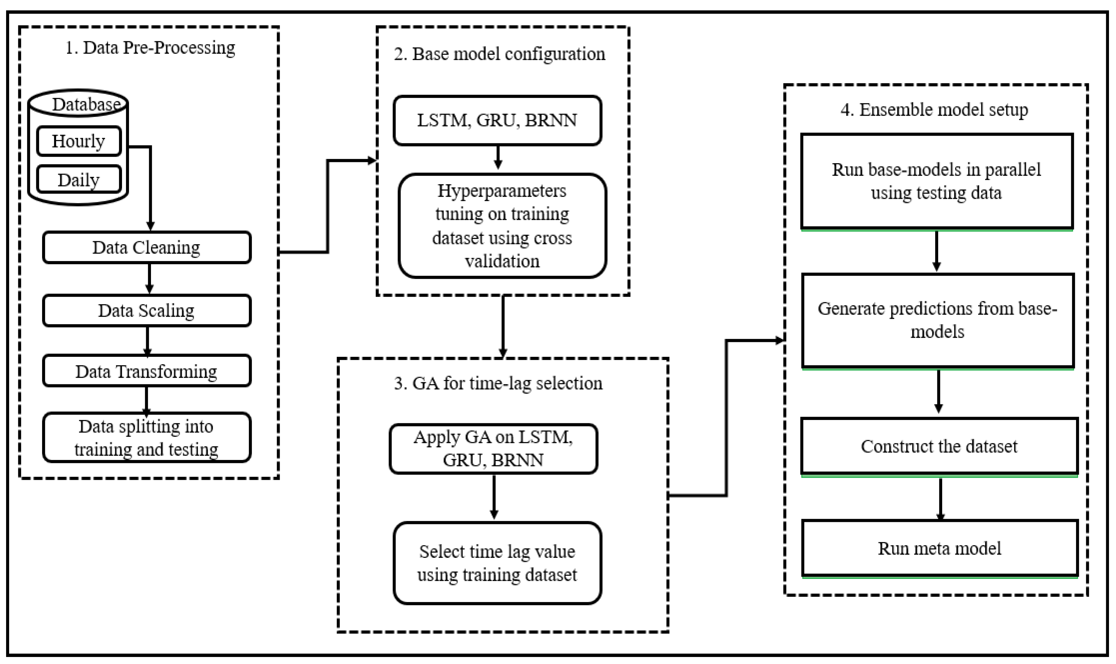
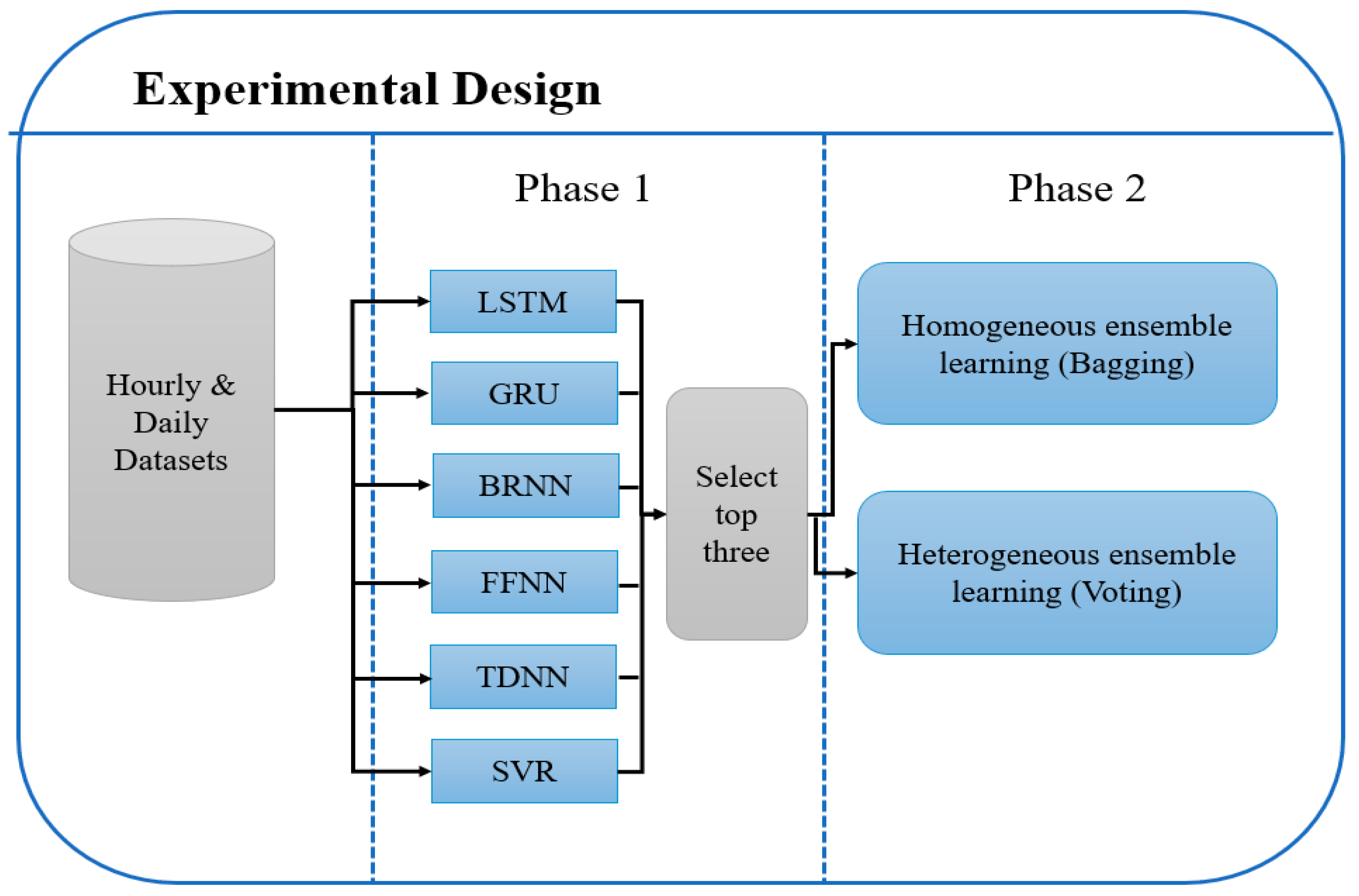
2. Materials and Methods

2.1. Database, Handling, and Preprocessing

The aerosol database used in this study was adopted from the measurement (1 August 2016–31 July 2017) carried out at the Aerosol Laboratory, which was located on the third floor of the Department of Physics, University of Jordan [21]. Amman is considered an example of Middle Eastern urban conditions. The Middle East region attracts the attention of atmospheric modelling researchers, as it serves as a compilation of aerosol particle sources including natural dust and new particle formation.
This database consists of particle number concentrations (PN) and local weather conditions (Temperature (T), Absolute Pressure (P), Relative Humidity (RH), Wind Speed (WS) and Wind Direction (WD)). The details of the aerosol measurements campaign and the metrological measurements lie beyond the scope of this paper, and detailed descriptions can be found in previous studies [21,22].
The database was processed into two databases (daily and hourly averages). The daily database contained 366 samples, and the hourly database contained 8784 records. Typically, a time-series database requires some preparation prior to being modelled with ML methods. The pre-processing sub step involves three main phases: Checking, Scaling and Transformation.
  • Checking: The database contained some missing data due to technical and instrumental issues. These missing values were replaced using the imputation method through interpolation. Each database became consistent with the expected number of records.
  • Scaling: The processed database was normalized because it is preferred to train the model with data values which fall within the same range as the activation function used in the model training. So, the scaling factor is dependent on the activation function. In this case, the data were scaled between 0 and 1 to transform it within the range of the neural network activation function.
  • Transformation: The data were transformed from a time-series form to a supervised form. The supervised data contained a sample with input and output components. The input component was a number of prior observations (defined by time-lag value). The output component contained the observation to be forecasted. In another words, the input was the observations from previous time steps, and the output was the observation of the current time step. The observation of the current time step became the input for the next time step, and so on.

2.2. Model Setup

The proposed model in this study was comprised of three ML methods: RNN methods (Gated Recurrent Networks (GRU), Long-Short Term Memory (LSTM), and Bi-Directional Recurrent Neural Networks (BRNN)), heuristic algorithm, and ensemble learning technique (stacking). The overall architecture of the proposed model is shown in Figure 1. The reason for choosing these methods can be summarized as follows:
  • Because it is a time-series forecasting problem, the prediction process can be accomplished using time-series methods such as RNN, which is able to capture temporal dependencies between data to produce more accurate results. Other methods can be used, such as Artificial Neural Network (ANN) and Bayesian Optimization methods, but these methods may cause overfitting as the time-lag feature is not taken into account. In the time-series data, the proper selection of time-lag value can reduce dimensionality of the non-linear data and avoid overfitting.
  • The proper selection of time-lag can improve model performance and generate a more accurate result. The time-series data can be viewed as a set of equal chunks where the records of each chunk are correlated and consistent. Finding the number of records at each chunk represents time-lag value, which is a difficult problem to solve and requires the running of several experiments to search for the best value that may generate the best prediction accuracy. Repeating this process has a high computational cost and consumes the resources. Using a heuristic algorithm to solve search problems is highly preferable by researchers as it can find the optimal solution (or near optimal) in a reasonable time with less computational cost. GA is used in this paper to enable us to find the optimal time-lag and prevent overfitting, increase model accuracy and generate the prediction with less computational cost compared to other heuristic algorithms.
  • More accurate results can be achieved through the use of ensemble technique, which combines the result of each single model to improve accuracy. The prediction result of ensemble method is usually better than the prediction of a single model. Heterogeneous ensemble learning is used in this paper, as different base models are used with different hyperparameter tuning.
The proposed model consisted of four main phases: (1) database pre-processing, (2) base model configuration and tuning, (3) GA operation, and (4) ensemble model setting. In the pre-processing phase, the database was first checked, scaled, and transformed. Then it was split into two main parts: training set and testing set. The percentage of the splitting process was 80% training and 20% testing. The training database was used to build a model, where the testing database was used for validation. In the second phase, the 10-fold cross validation method was applied on the training database for each RNN, LSTM, GRU, and BRNN along with the pretraining method. The time-lag value was set to 1, and the best combination of each method hyperparameters was selected. Pretraining involved adding a new hidden layer to the existing model and refitting. The new model would learn the input from the existing hidden layer while keeping the weights of it unchanged. This technique is called layer-wise which allow the adding of new layer at a time. As the solution was aggregated from the local optimal solution, it was called greedy. The optimal parameters of each network were considered where the configurations differ from hourly and daily databases. In the third phase, the GA was applied on each network to find the optimal time-lag after tuning each model (LSTM, GRU and BRNN) to achieve better performance of the model.
The time-series forecasting problem used lag to make a prediction based on the past observations of that lag. The choice of the appropriate time-lag value was an important step to ensure the generation of high-performance predictions in terms of accuracy. Time-lag could capture dependencies between successive time observations in the model. Because there is no general rule that specified how the lag variable can be selected [23], different approaches have been used by researchers in different application domains. The selection of the value that guarantees the optimal solution with high precision and generation is a complex problem that needs to run and repeat many experiments in order to search for the best solution. On the other hand, running these methods requires more time to find the optimal time-lag value that generates the best prediction, which exhausts resources and requires more time, so using a non-deterministic polynomial (NP) is difficult.
In order to solve the above-mentioned issue, a heuristic algorithm was used. The GA is an evolutionary algorithm that has been used by many researchers in the computer science field to solve complex problems in a variety of domains where the solutions of these problems cannot be found in a reasonable timeframe. Because it is easy to implement, is a global heuristic search algorithm, and can generate more accurate results, GA has become one of the most popular algorithms [24]. Previous studies have shown that GA can produce solutions that are near optimal solution, and it has been applied previously to optimize neural network configurations such as network weights and the architecture [25,26]. Comparing the performance of GA with other heuristic algorithms on solving different kinds of complex optimization problems, several studies show that GA performs better in obtaining the optimal solution, and is faster than other methods such as Differential Evolution (DE), Particle Swarm Optimizations (PSO), Ant Colony Optimization, and others [27,28,29,30]. GA has been applied widely in many applications from ML, Mathematics, Business, Robotica, etc., because they have the following advantages in solving complex problems in different domains [31,32,33,34,35]:
  • Robust and strong;
  • Non-deterministic algorithm and can be used for a variety of problems;
  • Works with the string-coded of the variables rather than the variable itself, so the coding discretizes the search space even if the function might be continuous;
  • An optimal solution could be generated by GA as it works with more than one solution (population).
In this paper, GA was applied in each RNN model to search for the optimal time-lag value. The training database was split into two sets, training and validation set. The GA was applied on the training set, while the validation set used to estimate the model performance on the time-lag value.
The population size was set to be 50 for both hourly and daily databases. Each solution represented the number of the lag value. The initial population was generated randomly. Next, the solutions were evaluated according to the fitness function. Each database was prepared according to the chosen time-lag value, and the network was trained (LSTM, GRU or BRNN). The results were then generated. MAE was calculated and returned as a fitness score to each current solution. The three GA operations were performed (selection, crossover and mutation), and the process was repeated for a number of iterations. At the end, the solution with the best fitness value score was selected as the best solution. The details of applying GA on each RNN method to find the optimal time-lag value are as follows:
  • Initial population: A binary vector randomly initialized the use of the uniform distribution defining initial solution. The population size was set to have 50 possible solutions.
  • Selection: Select the parents from population with the best fitness value.
  • Crossover: Exchange the variables between selected parents to generate new offspring. One-point crossover was used for that.
  • Mutation: A binary bit flip with probability of 0.1 was applied to the solution pool by randomly swapping bits to achieve diversity on the solutions.
  • Fitness function: MAE was used to evaluate solution.
The final phase of the proposed model is building the ensemble model, where the output from RNN methods with its different selected time-lag was run in parallel to generate outputs that were then combined with each other to produce the final PN concentration estimation. In this paper, the stacking ensemble model was used. It involved the combination of the predictions from multiple and different models on the same database. The stacking ensemble consisted of two main levels:
  • Level 0 (base models): Used three models (LSTM, GRU and BRNN) with selected time-lag value proposed by GA. The testing database was divided into 5 folds that were disjointed and of equal size. One fold remained aside, while others were used to train each model. The prediction was then made using holdout fold. More robust results are generated for each model.
  • Level 1 (meta model): Took the output from level 0 as an input to a single model called a meta-learner to produce the prediction output. A new training database was constructed from the predictions of sub-models where the first column contained predictions generated by LSTM. The second column contained predictions generated by GRU; the third column contained predictions generated by BRNN; and the last column contained the actual expected output. This way, a new stacked database was constructed. A ML algorithm is then used to learn how to best combine the prediction of sub-models. It is the meta-learner that uses a new stacked dataset for training.
To evaluate the effectiveness of the proposed model, three metrics were used: Root Mean Square Error (RMSE), Mean Absolute Error (MAE), and coefficient of determination (R2). These metrics can be formulated as follows:
RMSE   = ( 1 n   i   =   1 n ( y i y ^ I ) 2 )
MAE = 1 n   1 n | y i y ^ i |
R 2 = 1 ( y i y ¯ ) 2 ( y i y ^ ) 2
where n is the number of observations, y is the vector of the observed values and y ^ is the vector of the predicted values. RMSE gives the square root of Mean Square Error (MSE) that measures the average of the square of the error. MAE Measures the average absolute error of the paired predicted values from the original ones. It gives the magnitude of the overall error. R2 gives an indication of how strong the relationship is between the dependent and independent variables of the model.

2.3. Computation Setup and Platform

The work was implemented using Intel (R) Core™ i7-8550U CPU @ 1.80 GHz 1.99 GHz, 8.00 GB of RAM (Intel Corporation, Santa Clara, CA, USA) and Windows 10 version 1909 (Microsoft, Redmond, WA, USA). The application program was written in Python language and executed on JetBrains PyCharm Community Edition 2019.2 ×64. Python provides a set of libraries that can be used to create deep learning model directly, such as Scikit-Learn and TensorFlow. Scikit-Learn library provides a set of supervised and unsupervised learning algorithms that can be used and experimented directly. Table 1 summarizes the toolboxes and packages used.

3. Results and Discussion

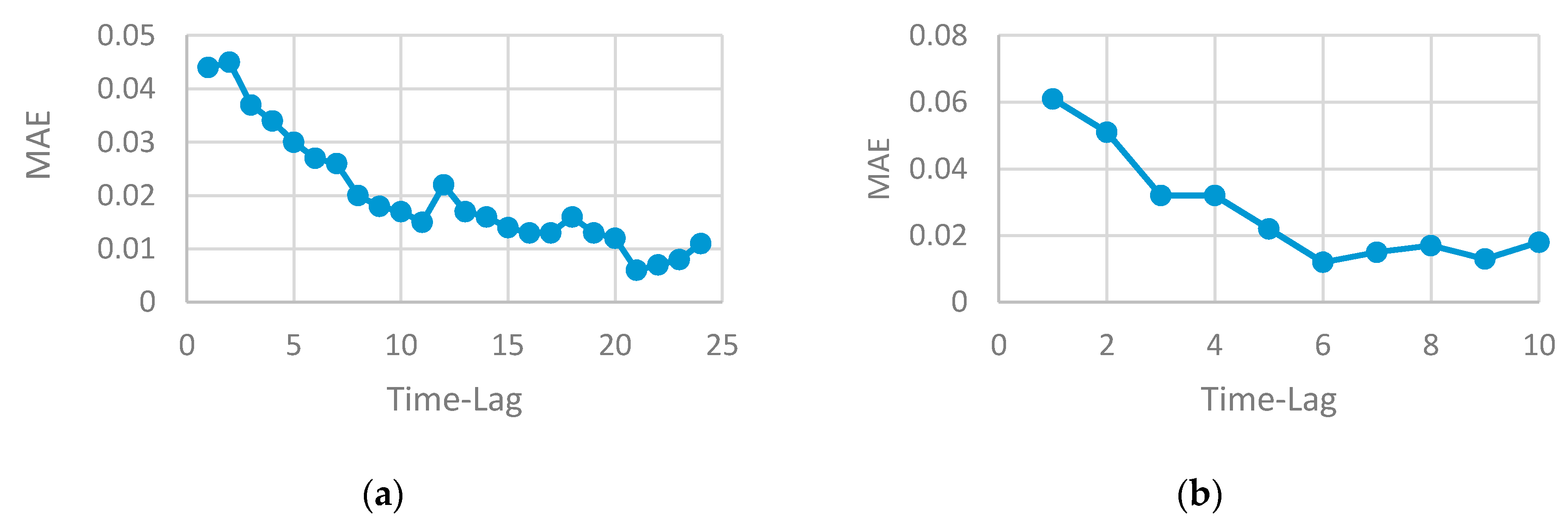
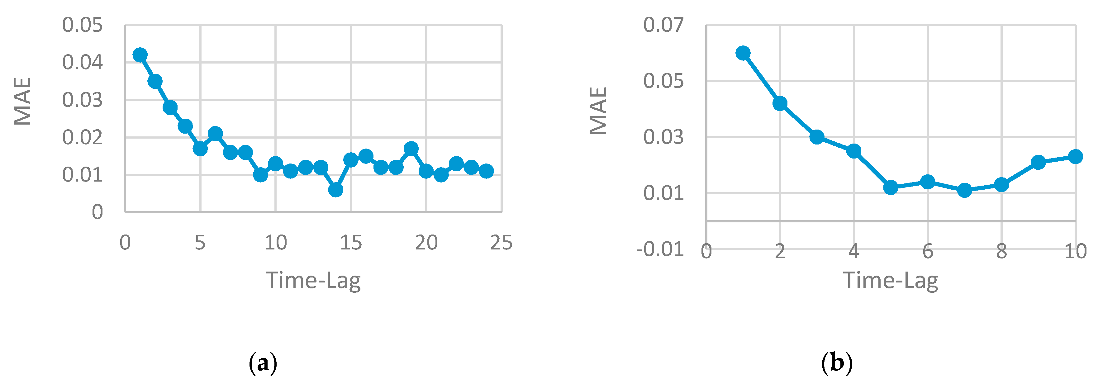
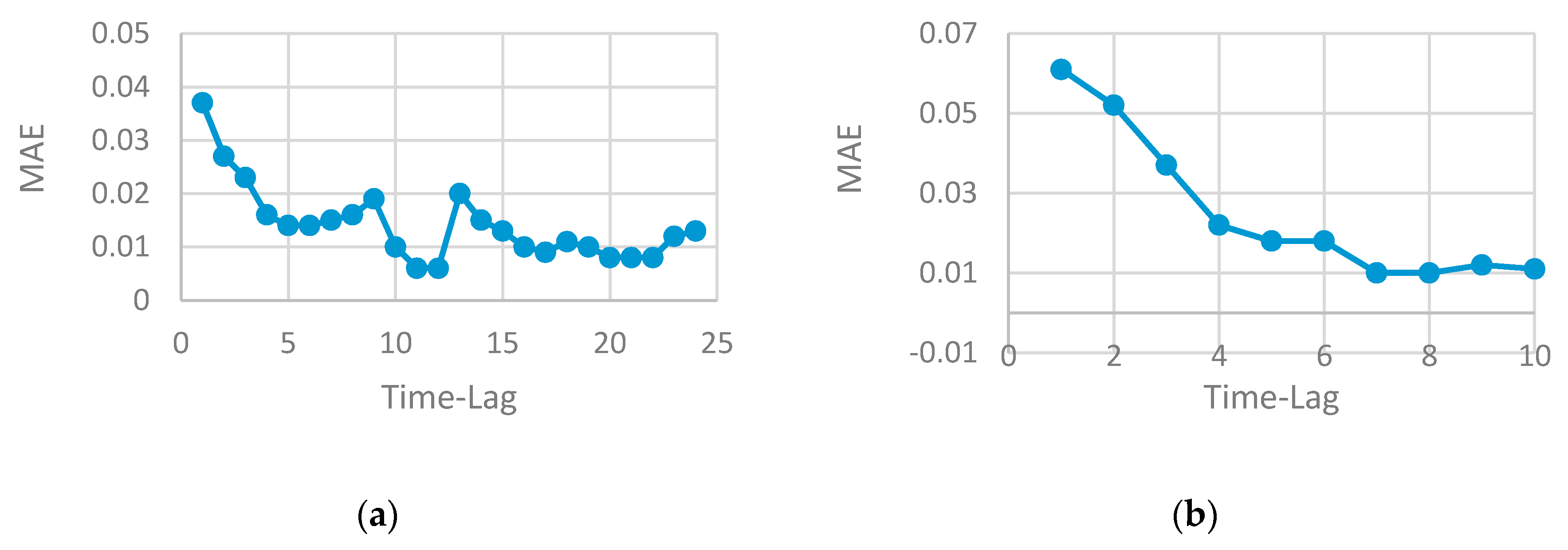
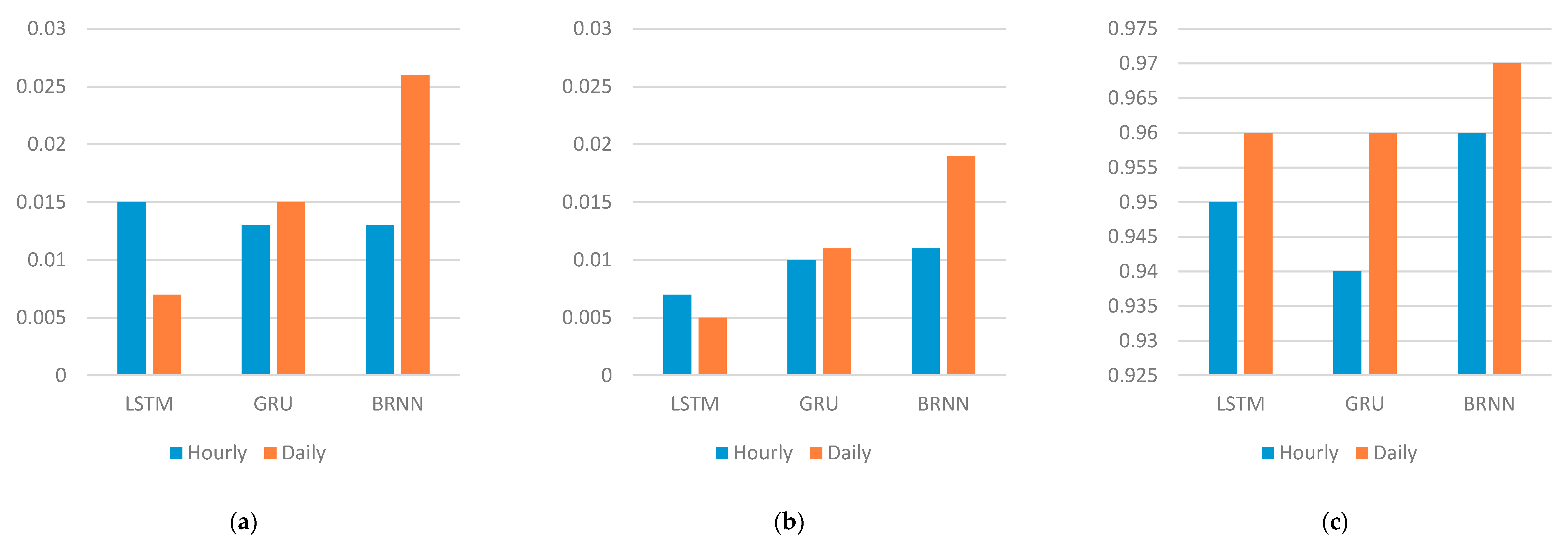
3.1. RNN Models—Evaluation and Performance

Applying 10-fold cross validation into each RNN method (LSTM, GRU and BRNN) results in tuning the network with the optimal set of parameters that generates best prediction. The values of each network parameter found by cross validation search optimization for both hourly and daily databases are given in Table 2. The generated solution from GA was used to train each RNN model and then was validated. The solution that gives the best fitness score was selected as the best time-lag value and was used in the network configuration (Figure 2, Figure 3 and Figure 4).
Analyzing the results generated from the application of GA on LSTM, GRU and BRNN shows that a different lag value was selected for each method and each database. The performance of each algorithm differs regarding to the running time and accuracy. All methods performed better as the number of the time-lag value was increased. For a small time-lag value, the BRNN performed better and generated a smaller MAE value when compared to LSTM and GRU. The BRNN method also performed better than LSTM and GRU in terms of accuracy (i.e., MAE value) when the running time of this algorithm was extended. The backward and forward run of BRNN enhanced prediction performance, but increased the running time. LSTM and GRU were comparable to one another’s, regardless of the time-lag value suggested by the GA to be the optimal value. Table 3 lists the best time-lag value selected by GA for each RNN method along with the running time (in minutes) needed to generate this result.
The configuration of each RNN model chosen from the cross-validation process along with an appropriate time-lag value selected by GA was used to construct the stacked ensemble model and generate the final prediction. The three methods were run in parallel using multi-cores in order to enhance running time performance. The testing database was used to train each base model, the out-of-sample data generates the predictions. The results of level 0 from the stacked ensemble model are given in Table 4 and shown in Figure 5.
An enhancement in the model performance was achieved in terms of speed by the parallel implementation. It took 25.05 min to finish the training and make a prediction for the three methods. The stacking ensemble technique was preferred when multiple models with different skills were used to train the same database, and each model may behave in a different way.
For both databases (i.e., hourly and daily), the LSTM outperformed GRU and BRNN in terms of RMSE and MAE metrics (Figure 5). The running time of BRNN was more when compared to LSTM and GRU, due to the forward and backward architecture of BRNN. The GRU method, which had a similar architecture to the LSTM, was less effective than LSTM. This was due to the architecture of the GRU, which had fewer gates than the LSTM. Capturing the time dependency between series observations was not as accurate as with the LSTM method; this result was concluded from the R2 value of GRU, which was the lowest on the hourly database.
The output of each method was used to construct a stacked database. The new database was used to train the ANN model (meta model) and generate the final prediction results. In order to show the enhancement achieved by the ensemble model in terms of prediction accuracy, Table 5 shows the accuracy generated by each base model (LSTM, GRU and BRNN) and the ensemble model for the hourly and daily databases.
The ML methods used in this paper were supervising learning methods. These kinds of methods can be clearly analyzed using bias and variance trade-off. As the goal of any supervised learning method is to best estimate the mapping function (f) for the output variables (y) given an input variable (x). The prediction is then generated and the error is estimated. The error can be broken into two parts: bias and variance. The bias error is the prediction error. It reflects the distance between the actual and predicted values, and can be estimated by finding MSA, RMSE, etc. The variance error reflects the amount of change in the prediction accuracy if different training data are used.
The ML algorithm with high variance was highly influenced by the specific training data. This means that these data influenced the choice of parameter types and numbers used in the network training to characterize the mapping function. A good ML algorithm has a low bias and low variance. Through this, it generalized the error and achieved a good prediction performance. The parameterization of the ML algorithm to reduce bias and variance was often difficult, especially when working with non-linear algorithms such as neural networks.
In this paper, the results of modelling time-series data using a heterogenous ensemble learning model that is composed of three different variants of RNN method—LSTM, GRU and BRNN—can be summarized as follows:
  • The performance of any neural network depends on the parameters tuning. The good selection of each parameter (such as the number of neurons, the number of layers, the number of time-lag, etc.) can either increase or decrease accuracy. Finding the optimal selection of network parameters is an NP problem that requires repeating the experiment by changing one parameter while keeping the other fixed. Determining the set of parameters that influence the network performance depends on the problem domain and the type of data. In this paper, time-series data are used where the RNN method is well-suited to be applied. The number of lags is a very effective parameter that can increase or decrease the model accuracy. The use of a heuristic algorithm in the proposed work searched for the best value of the time-lag to be chosen for each network architecture. This selection guarantees the use of the best value, that produces a robust model and enhances accuracy.
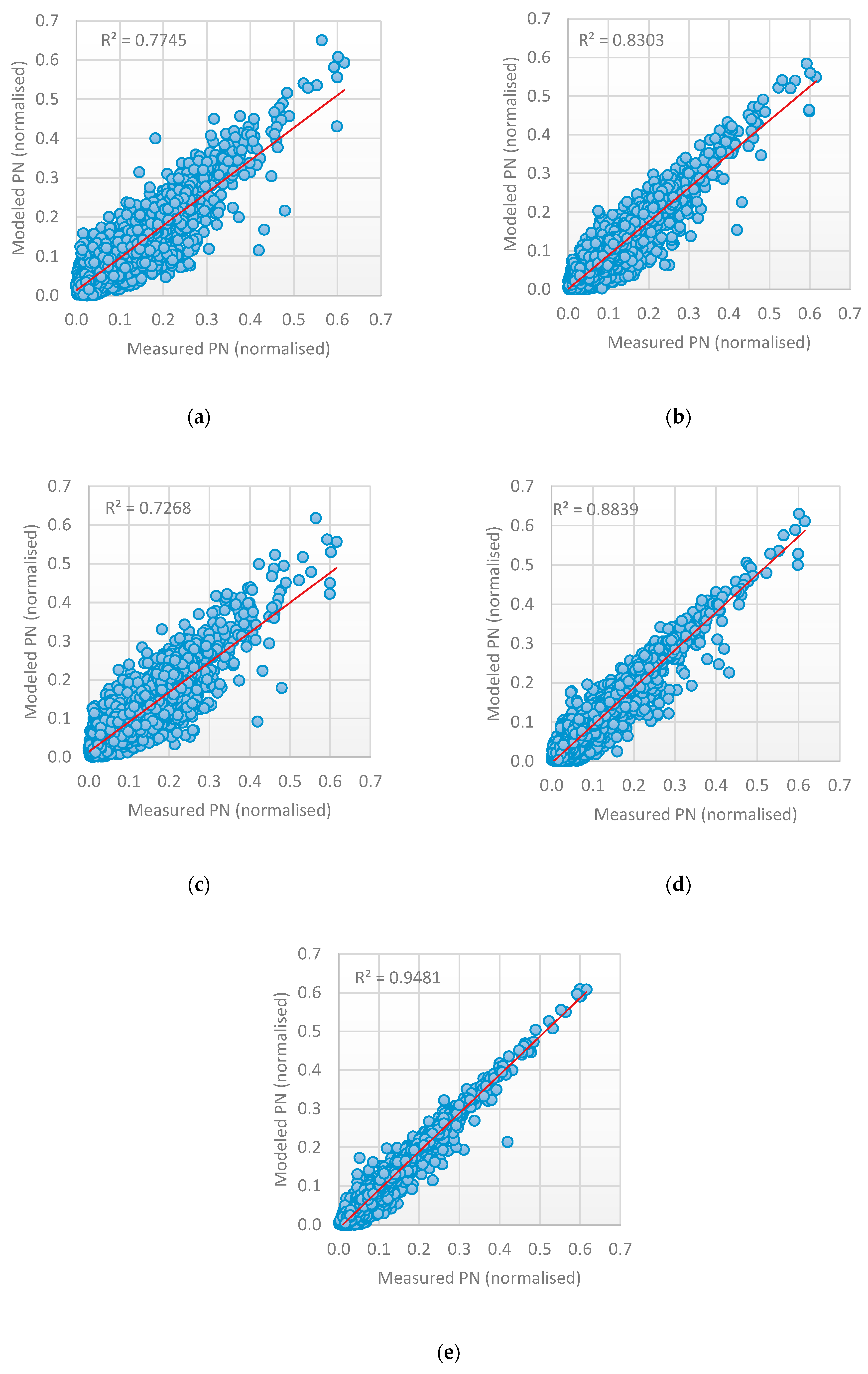
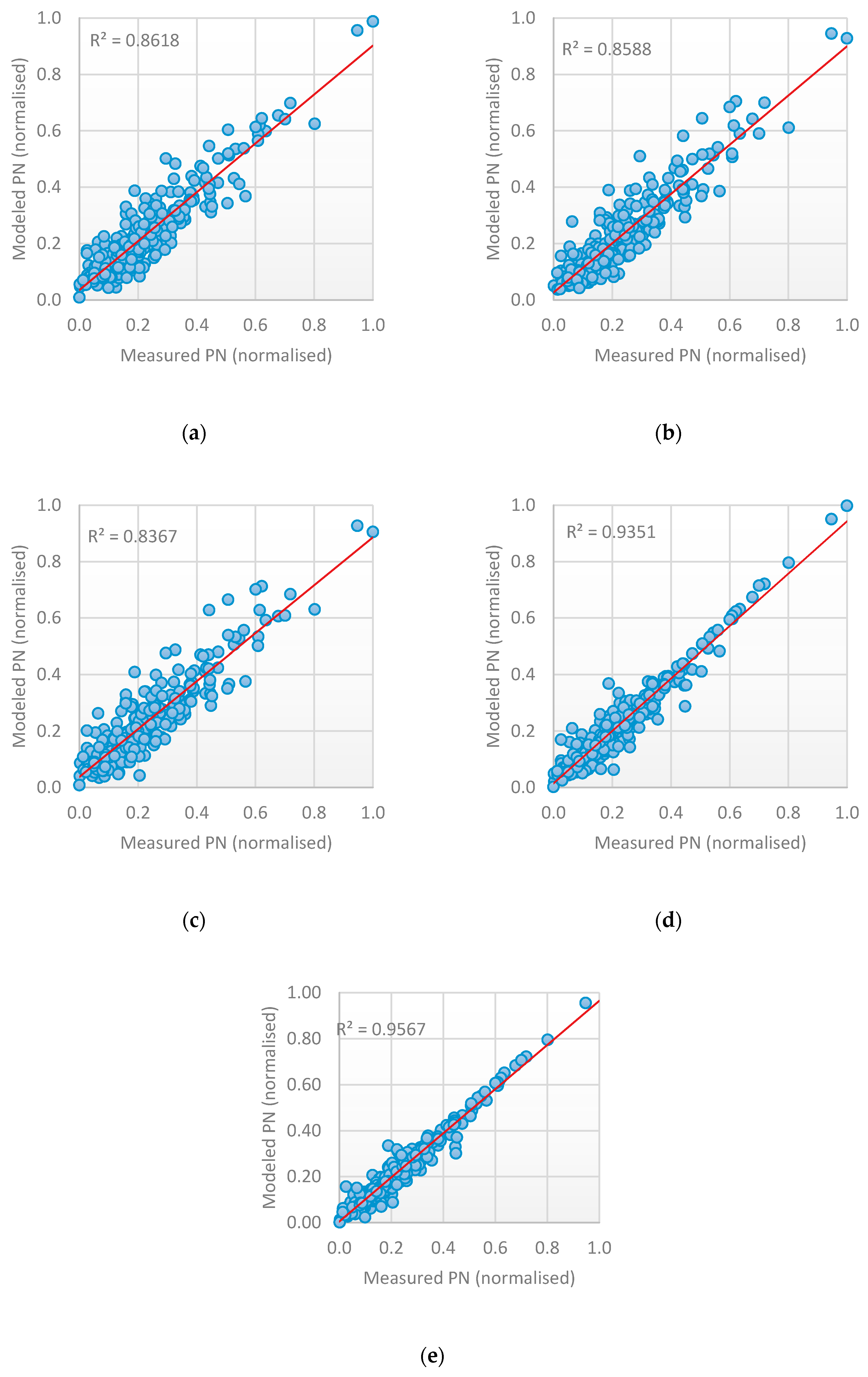
  • A recurrent neural network is the best method to be used to design a predictive model for time-series data. Many variants of RNN have been developed in the literature where each version has its advantages and disadvantages. The three selected RNN methods used in this paper are LSTM, GRU and BRNN. Three models are designed using each method. The results can be summarized as follows:
    (a)
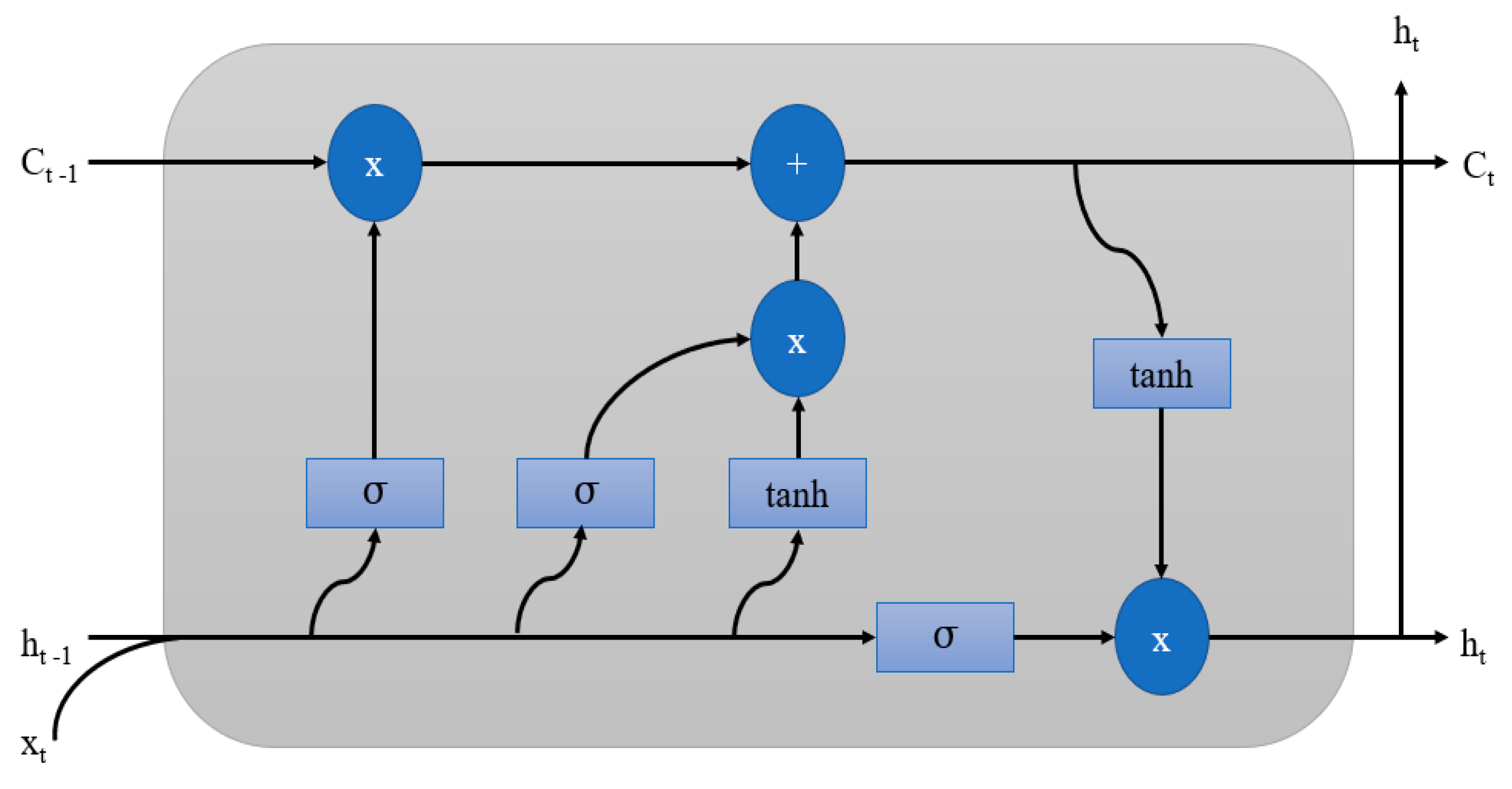
    LSTM model is accurate, robust and efficient. For a large amount of data, LSTM needs more time to generate an accurate prediction.
    (b)
    GRU is simpler than LSTM. On the other hand, it is less accurate, although the time needed to run a GRU model is less than the LSTM running time.
    (c)
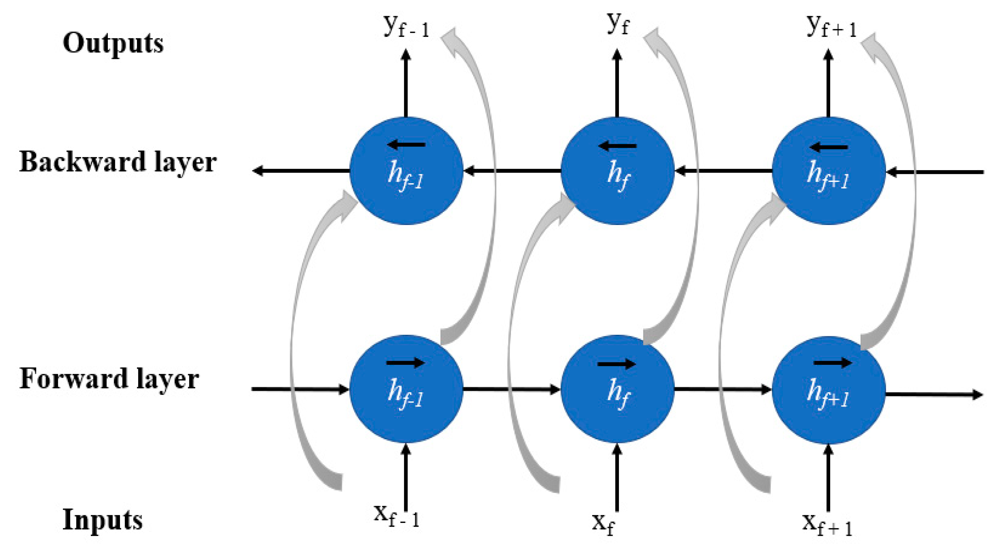
    BRNN is accurate and robust, but it needs much time to produce a prediction on account of its backward and forward architecture.
  • The number of the time-lag has a great effect on the algorithm performance for time-series data. Increasing the time-lag value (window size) increases the running time of the model.
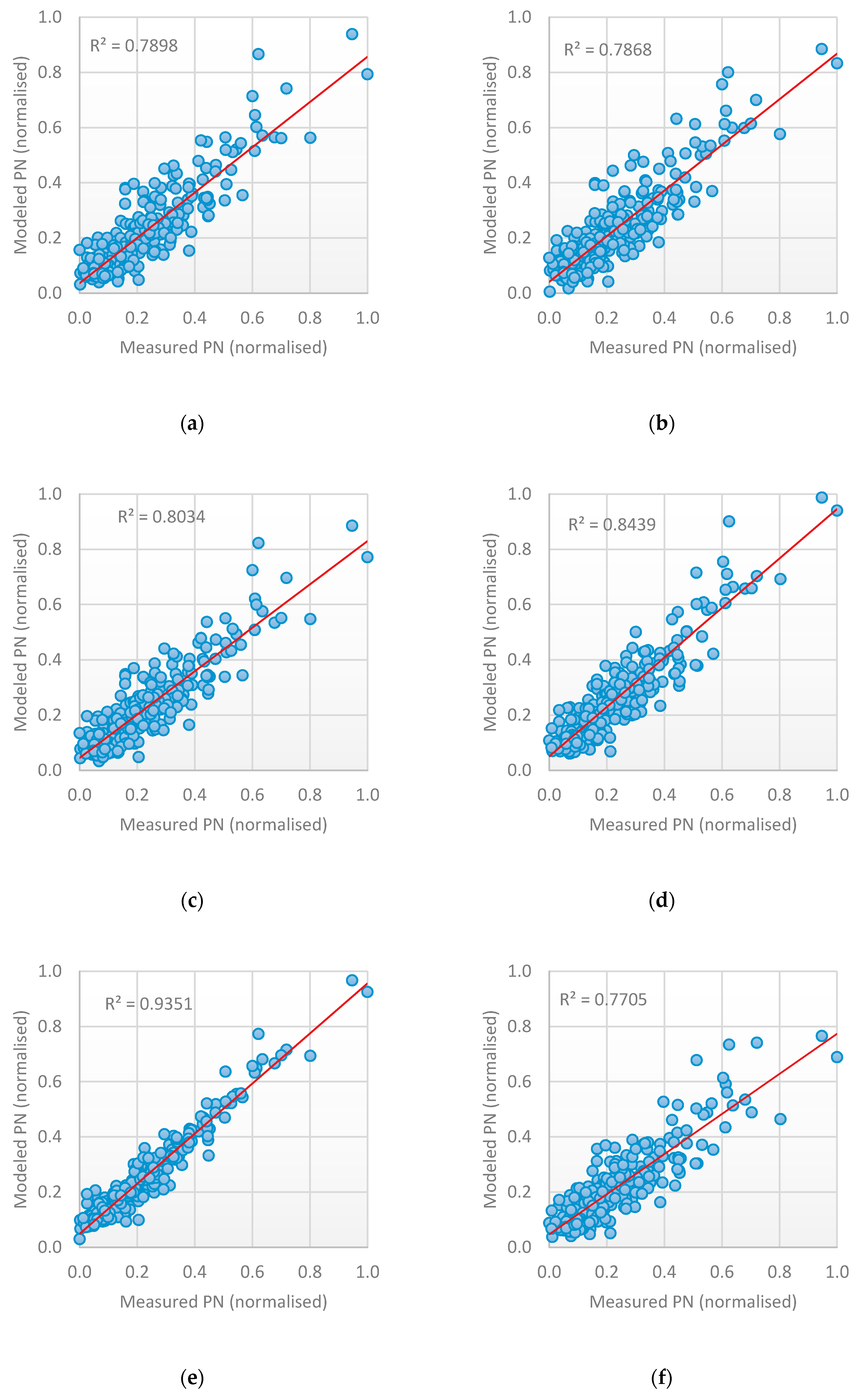
  • An improvement in the prediction accuracy can be achieved by combination of the result of each method to produce a final one. This is achieved by designing stacked heterogenous ensemble learning that combines the output of each RNN method and uses a new learner to generate the final output. The ensemble learning technique improves accuracy, and the parallel implementation reduces running time. Having three base-learners with a different time-lag number and different architecture reduced error generalization and overfitting, and increased diversity, as shown in Table 5.
  • The parallel implementation of ensemble method enhances model performance, by reducing time needed to make the prediction.

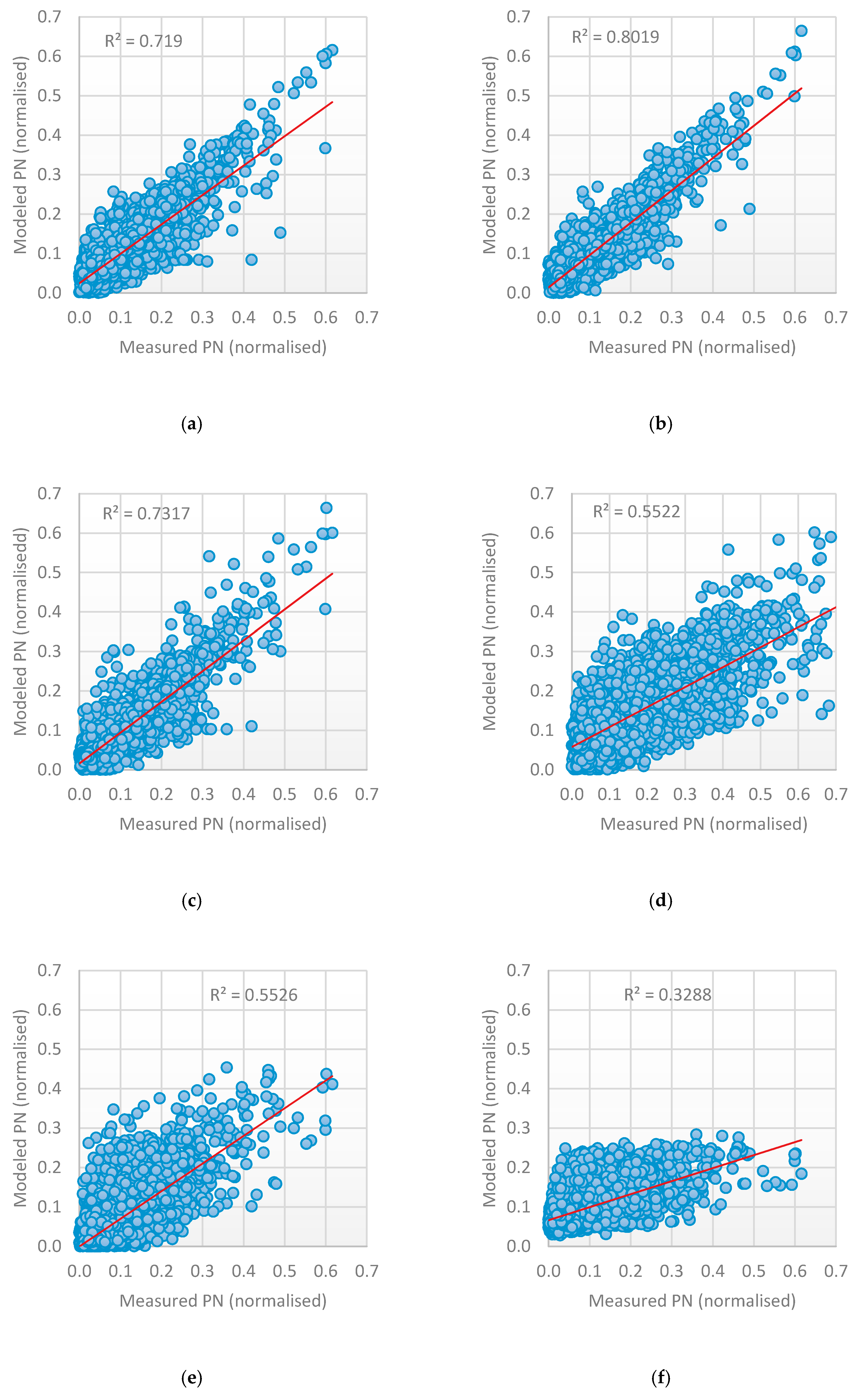
3.2. Comparison with Other and Previous Methods

The model performance and accuracy were compared with previous and other methods. Zaidan et al. [18] proposed a framework using an Artificial Neural Network (ANN) to model PN concentrations in Amman, Jordan (i.e., the same data used here). Different sets and combinations of all weather parameters were the descriptors used. According to their results, the best combination was including the five weather parameters, which were then compared with the results produced in this paper using LSTM, GRU and BRNN with time-lag value equal to 1 (Table 6). It is evident that our new approach (i.e., LSTM, GRU and BRNN) outperforms the previous one (i.e., ANN). Besides that, ANNs require an optimum network structure with optimum configurations to avoid overfitting and achieve better accuracy; this requires running several epochs, resulting in a long training time. Therefore, it can be said that for a time-series application, it is recommended to use a time-series model based on the use of RNN to achieve better prediction and accuracy.
We also compared the current approach with other ensemble approaches, which were based on Bagging and Voting representing heterogeneous and homogeneous ensemble techniques. The experiment was divided into two main phases: (1) six benchmark learning algorithms that were trained over two databases (i.e., hourly and daily), and (2) three ensemble models (bagging, voting and stacking) (Figure 6).
In Phase 1, the performance of LSTM, GRU and BRNN was compared with other benchmark ML algorithms. The selected algorithms were Feed-forward Neural Network (FFNN), Time Delay Neural Network (TDNN), and Support Vector Regression (SVR). The results had six ML algorithms that were used as base learners. This main task accomplished through this phase was to prepare each algorithm by tuning it for training. The performance of each algorithm was investigated using a 10-fold cross validation and the Greedy layer-wise pretraining technique, where the accuracy of them all was compared. The best three algorithms were used to construct the homogeneous and heterogenous ensemble method (i.e., Phase 2). Here, the time-lag value was not investigated in this experiment and was set to 1; in fact, the effect of choosing a proper time-lag value has been sufficiently investigated using GA. The prediction accuracy results for each of them were evaluated using the same evaluation metrics—RMSE, MAE and R2. In Phase 2, we constructed the ensemble learning algorithms as follows: (1) selected the top three most accurate algorithms in Phase 1; (2) developed a homogeneous ensemble learning method (i.e., Bagging); (3) developed a heterogenous ensemble learning method (i.e., Voting); and (4) the results of the homogenous and heterogenous ensemble models were compared with the current model (i.e., using stacking ensemble). The results generated in Phase 1 are presented in Table 7. The main aim of this phase was to conduct and compare the performance of each base learner algorithm (LSTM, GRU, BRNN, FFNN, TDNN and SVR) over two databases (hourly and daily) in terms of three evaluation metrics (MAE, R2 and RMSE). Figure 7 and Figure 8 show the prediction scatter graph for PN concentrations using six base learner algorithms over both databases.
According to the models performance in Phase 1, the current method (i.e., three variants of the RNN models) outperformed the other three base learners (i.e., FFNN, TDNN and SVR) for the hourly database (Table 7 and Figure 7). This result shows that LSTM, GRU and BRNN can handle the high dimensionality of the non-linear hourly database and capture correlation between independent variables and the dependent variable (input and output). LSTM, GRU and BRNN can be also used to construct voting and stacking ensemble models. FFNN, TDNN and SVR can be used to construct the bagging ensemble model. As for the daily database (Table 7 and Figure 8), the TDNN method performed the best, and SVR was the worst. Consequently, the best base learners (i.e., TDNN, FFNN and BRNN) were used to construct the heterogeneous ensemble learning model (voting and stacking). The worst base learners (i.e., SVR, LSTM and GRU) were used to construct the homogeneous ensemble learning model (Bagging). The performance and accuracy using the homogeneous and heterogeneous runs are presented in Table 8 and Figure 9 and Figure 10. Many studies have been carried out for time-series prediction and using ensemble models. When compared to those methods, the current model is robust (Table 9).

4. Conclusions

Time-series prediction is an important area for many applications. Using state-of-the-art ML methods, such as ensemble learning and Recurrent Neural Network (RNN), can improve the prediction accuracy and enhance the results. In this paper, we proposed a new approach that consists of four main phases to predict particle number concentrations in the form of a time-series prediction. The first step was to perform data pre-processing and split into two parts: a training set and a testing set. The training database was used to build the model. The testing database was used to construct the ensemble model. The RNN base learner models were fed by using training data, and each network was configured using 10-fold cross validation. The optimum configuration of each network was considered and tested. Then, the Genetic Algorithm (GA) was applied on each network to find the most optimal time-lag. The final phase of the proposed method was to establish the ensemble model using a testing database, where the output from RNN method with its different selected time-lag was run in parallel to generate outputs that were combined with one another to produce a final PN concentration estimation.
The results demonstrated that LSTM, GRU and BRNN were suitable techniques for time-series modelling, as they were found to be robust and accurate. Among them, LSTM was the best, but requires more time to process a large amount of data. The number of the time-lag values had a great effect on the algorithm performance for time-series data. A different time-lag value was selected by the heuristic algorithm for each learning method. The selected lag value generated the best accurate result. A stacked heterogenous ensemble learning method that combines the output of each RNN method and uses a new learner to generate the final output was constructed. The ensemble learning technique improved accuracy, and the parallel implementation for base learner methods reduced running time. Having three base-learners with a different time-lag number and different architecture reduced error generalization and overfitting, and increased diversity.
As a recommendation, we state the following points for future research:
  • An improvement in the prediction model can be achieved by including more data with different features, such as the use of air quality image data. A combination between Convolutional Neural Network and Recurrent Neural Network can provide a more robust and high precision predictive model.
  • Parallelize neural network models by dividing the single neural network algorithm into tasks where each task can be run in a single core. The running time of the neural network can be reduced, and the performance will be enhanced in terms of speedup.
  • Various optimization parameters can be tested and investigated to improve accuracy such as the learning function and network structure.

Author Contributions

Conceptualization, O.M.S., M.A.Z. and T.H.; methodology, O.M.S., M.A.Z. and T.H.; software, O.M.S.; validation, O.M.S., S.S., M.A.Z. and T.H.; formal analysis, O.M.S.; investigation, O.M.S. and T.H.; resources, T.H. and M.A.Z.; data curation, T.H.; writing—original draft preparation, O.M.S.; writing—review and editing, O.M.S., M.A.Z., S.S., I.S. and T.H.; visualization, O.M.S.; supervision, S.S., I.S. and T.H.; project administration, T.H. and M.A.Z.; funding acquisition, T.H. All authors have read and agreed to the published version of the manuscript.

Funding

This research was funded by the Scientific Research Support Fund (SRF, project number BAS-1-2-2015) at the Jordanian Ministry of Higher Education and the Deanship of Academic Research (DAR) at the University of Jordan. This research was part of a close collaboration between the University of Jordan and the Institute for Atmospheric and Earth System Research (INAR/Physics, University of Helsinki) via the Academy of Finland Center of Excellence (project No. 272041) and Center of Excellence in Atmospheric sciences and NanoBioMass (project number 1307537).

Acknowledgments

Open access funding provided by University of Helsinki.

Conflicts of Interest

The authors declare no conflict of interest.

Appendix A. Recurrent Neural Network (RNN)

RNN provides a robust approach for time-series prediction, because it can handle high dimensionality non-linear data by the proper selection of time-lag values. In this paper, we utilized an heuristic algorithm to guarantee the proper selection of a lag value which improved the accuracy of the model prediction. Three RNN methods were used—LSTM, GRU and BRNN. Each RNN model was optimized and tuned using a cross-validation method. The model that generated the best results was used with its setting parameters. Greedy layer-wise pretraining was used to optimize the building of deep neural network to achieve state-of-the-art performance.
An heuristic algorithm was used to investigate the effect of time-lag values in each RNN model. The GA was a search optimization algorithm used to find the optimal solution within a given search space. Each base model used a different time-lag as selected by the GA. This enabled the model to see enough past values that were relevant to the future prediction for more accurate and stable forecasting.
Further improvement in accuracy was achieved by using the ensemble learning technique. This involved the use of multiple models that were trained independently, and the output of all models was combined using a specific technique to improve the accuracy of the prediction task. The ensemble network could be homogeneous or heterogeneous. In the homogeneous ensemble, all models were of the same type but with different structure. The heterogeneous ensemble contained an identical independent model structure where each model was trained with different training data. The optimization of time in terms of computation time was achieved by using parallel implementation for the proposed ensemble learning model, where the three base learners used in the ensemble model were run in parallel on a multicore platform.
In the real-world, time-series forecasting (e.g., air quality and weather) involves complex nonlinear relationships between multiple variables. Traditional forecasting approaches have limitations related to [14]:
  • Missing data and outliers. For example, some statistical models (e.g., Support Vector Machine (SVM)) are sensitive to missing data and the forecasting accuracy is affected.
  • Assumptions of linear relationship, which cannot deal with complex nonlinear relationships. For example, the ARIMA model can only describe the linear relationship between variables.
  • Number of variables in the regression equation. For example, the prediction accuracy of a regression model depends on the number of dependent variables. Increasing the number of variables improves the accuracy but increases the computation time.
In practice, ML methods are widely utilized in computer science, statistics, and neural computing. ML have many advantages: they can be used to describe the data characteristics without prior knowledge about their distribution; they depend on the data parameters to model application behavior; they are simpler than statistical methods to adjust; and show reliable performance when applied to non-linear and complex series. ML have some disadvantages: they are black-box models, and they use historical data to learn the stochastic relationship between past and future observations [40].
Neural Network (NN) models are the most popular type of ML method. They are based on a mathematical model that is inspired by the behavior of biological neurons. They are developed to learn the mapping from inputs to outputs over a long sequence of both structured and non-structured data [41]. They can handle missing data, model complex nonlinear relationships, and support multiple inputs.
In general, there are many models of NNs, starting from the Multiple Linear Perceptron (MLP) to the advanced deep learning neural networks that become a powerful tool of ML and artificial intelligence. Recurrent Neural Network (RNN) is the most popular used method for time-series data forecasting. The RNN structure consists of one input layer, one output layer and one hidden layer with one or more feedback loops [42]. The hidden layer in RNN contains states and a memory block where the state of the hidden layer at current time is conditioned with its previous state [43]. The memory block enables RNN to store, remember and process past data for a long period of time. A number of modifications to the original RNN architecture have been developed over the years. Some RNN variants include Long-Short Term Memory (LSTM), Gated Recurrent Network (GRU) and Bi-directional Recurrent Neural Network (BRNN), which are mainly used in the proposed model.

Appendix A.1. Long-Short Term Memory (LSTM)

Long-Short Term Memory is a type of RNN that is capable of learning a long dependency in sequence prediction problems [44]. When an RNN model fails to learn the data with a limited time-lag, LSTM is designed to address this problem by using specific units in its internal structure.
The architecture of LSTM consists of one input layer, one output layer, and a series of hidden layers that are recurrently connected and known as memory blocks (Figure A1). Each block consists of one or more self-recurrent memory cells in order to make it connected to itself, and three main units (input, output and forget gates). In each block, the three gates provide continuous read, write and reset operations; the interactive operations between three gates make LSTM sufficient to solve long-term dependencies that RNN cannot handle.
Figure A1. A schematic diagram for the Long Short-Term Memory (LSTM) structure. Here, t is the current time step, x is the input and σ is the activation function.
Computers 09 00089 g0a1
In the deep learning of neural networks, the gradient vanishing problem occurs when the previous hidden layer’s learning speed is slower than that of deeper hidden layers. This decreases the accuracy of the hidden layer learning [45]. The memory cells in LSTM make it better able to learn a long sequence with longer time steps. This makes it suitable to solve problems with time serial issues.

Appendix A.2. Gated Recurrent Networks (GRU)

Gated Recurrent Networks (GRU) are designed to learn with long-range dependencies [46]. GRUs are similar to LSTM in gating units; the information flow occurs with short memory and few gates (two gates, reset and update gate). The reset gate determines how to combine the new input with the previous data. The update gate indicates how much of the previous memory remains. Having fewer gates makes GRU faster at learning than LSTM. At each timestep, GRU exposes the whole state and computes the linear sum between the current state and the newly computed state [47].
It is important to keep in mind that both LSTM and GRU are efficient in predicting long-term dependencies. Both are used in state-of-the-art deep learning applications, such as speech recognition and natural language processing.

Appendix A.3. Bi-Directional Recurrent Neural Networks (BRNN)

In the BRNN, future context is used in the learning process and for the current prediction. BRNN considers all the available input sequences in the past and future to estimate output [48]. It processes the sequence in the two directions—forwards and backwards (Figure A2). In the forward direction, one RNN processes the sequence from start to end. In the backward direction, another RNN processes the sequence from end to start in a negative time direction. There is no interaction between the two RNNs. The output of forward direction is not used as an input to the backward direction, and vice versa. The challenge of using BRNN is the requirement to determine the start and end of the input sequence in advance.
Figure A2. A schematic diagram for Bi-Directional Recurrent Neural Network architecture. Here, x is the input, y is the output, h is the hidden node, and f is the activation function.
Computers 09 00089 g0a2

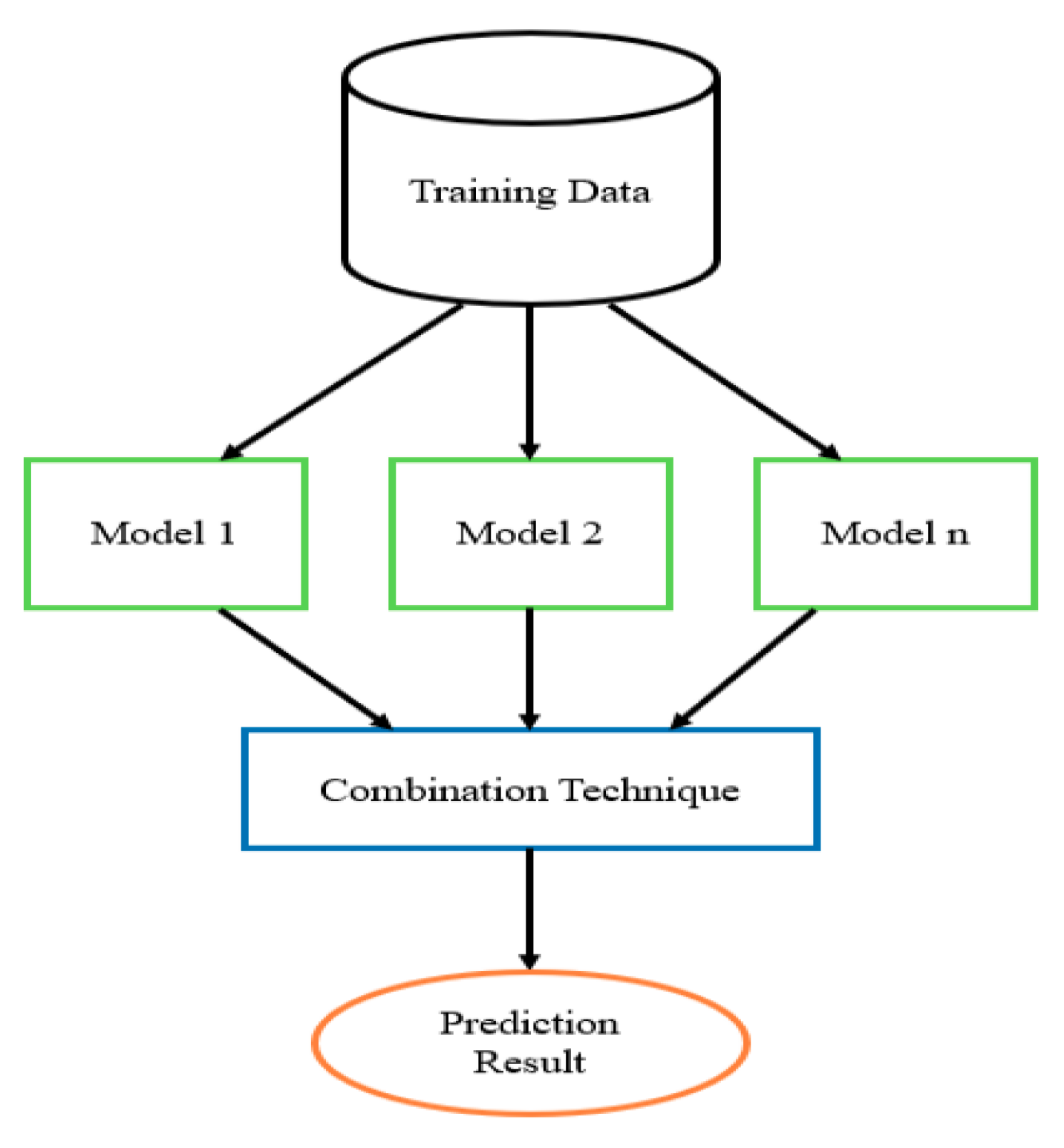
Appendix A.4. Ensemble Learner Algorithm

Ensemble learning is another ML method that is used to enhance learning accuracy (Figure A3). It is based on the use of more than one models (more than one base learner), that are trained with a given database to provide a solution for a given problem with a higher reliability and accuracy than what can be achieved using only one model [49,50,51].
Figure A3. Ensemble method framework [52].
Computers 09 00089 g0a3
There are three major elements in the ensemble technique:
  • The Training Data (i.e., problem database);
  • Ensemble Models (i.e., NN methods used as a base learner);
  • Combination Techniques (i.e., the way to produce the final prediction).
Changing any of the three ensemble elements affects the final prediction results. It is challenging to design the best combination of ensemble learning models to generate the most reliable and accurate results.
  • Training Data: The base learner models used in the ensemble method can be trained with the same problem database, or each model can be trained with a subset database that is different from the subset used with other learners. The k-fold cross validation method can be used to divide the database into samples where each base learner uses one sample for training. It is preferred that each base learner generates a result with a low correlation with results generated by other base learners to achieve a generalization in the model performance. Based on this, using different samples to train each base learner is preferred when constructing the ensemble model.
  • Ensemble Models: Selecting base learners that contribute to the ensemble architecture depends on the problem domain. In time-series data, RNN and its variants can be used to construct the ensemble model. The tuning of each base learner model becomes a challenge that influences its performance. When the ensemble model is constructed using the same kind of learning algorithm as for base learners (for example, a neural network), then it is called a homogeneous ensemble. If it is made up of more than one different learning algorithm, it is called heterogeneous [53]. When training the base learner models used in the ensemble design, each base learner model will have an error value that reflects its prediction accuracy. It is recommended to use models that result in a low correlation of error made by each model. This implies the tuning of each model with a different value of parameters.
  • Combination Techniques: At the end of training, the results are combined to produce the final prediction. There are many ways to do this:
    • Bagging: Dividing the database into samples where each one is fed to one base learner model. The final prediction is estimated by finding the average of each base learner model prediction. There are different bagging models, including Bagged Decision Tree, Random Forest and Extra Trees.
    • Boosting: Building a chain of base learner models where each one attempts to fix the error of the model that proceeds it. Common boosting models include AdaBoost and Stochastic Gradient Boosting.
    • Voting: Building an ensemble model with more than one base learner with some statistics (such as mean) to combine the final prediction.

Appendix A.5. Genetic Algorithm (GA)

In artificial intelligence and mathematical optimization, the heuristic algorithm is a technique used to solve complex problems in a reasonable timeframe where classic methods fail [54]. The solution provided by the heuristic algorithm may not be the best among other solutions, but it may simply approximate the exact solution.
Genetic Algorithm (GA) is a search heuristic algorithm that is inspired by natural evolution [55]. The algorithm reflects the process of natural selection, where the best individuals are selected from population to produce new offspring for the next generation [24]. The selection of parent individuals depends on a score assigned to each one in the population which is called “fitness value”. The process keeps iterating until a generation with the fittest individuals is generated. Five phases can be considered for GA:
  • Initial population;
  • Fitness function;
  • Selection;
  • Crossover;
  • Mutation.
The algorithm repeats the operations described above to a number of iterations that guarantee the generation of the optimal solution of the problem. For a given problem, the initial population can be defined to have a set of individuals, where each one represents a possible solution to the problem. Each individual is characterized by a set of parameters called genes. The joined genes form a chromosome (solution). There are different types of representation for solutions in GA. These could be binary, decimal, integers, and others. Each type is selected according to the problem and is treated differently. The fitness function gives a fitness score to each individual. Based on the fitness score, the ability of an individual to compete with other individuals can be determined, and the selection of an individual for reproduction depends on its fitness score.
Selection, crossover and mutation are the three main operations applied by GA to solve a given problem. The idea of selection phase is to select the fittest individuals in order to pass their genes to the next generation. The individuals with the highest fitness score are usually selected for reproduction.
Crossover is more significant; it selects a point for each pair of parents to be mated and makes crossover between them. The new offspring are generated by exchanging the genes of parents among themselves until reaching the point of crossover. The new offspring can then be added to the population. Crossover can be one point, two points, uniform, and others.
The mutation operation enhances the new offspring by flipping some bits in the offspring bit string. Mutation occurs to maintain diversity within the population, and prevents premature convergence. Mutation types are bit flip, inverse, uniform, non-uniform, and more.

References

  1. Chung, H.; Shin, K.-S. Genetic Algorithm-Optimized Long Short-Term Memory Network for Stock Market Prediction. Sustainability 2018, 10, 3765. [Google Scholar] [CrossRef] [Green Version]
  2. Bui, C.; Pham, N.; Vo, A.; Tran, A.; Nguyen, A.; Le, T. Time Series Forecasting for Healthcare Diagnosis and Prognostics with the Focus on Cardiovascular Diseases. In Proceedings of the Precision Medicine Powered by pHealth and Connected Health, Ho Chi Minh, Vietnam, 18–21 November 2017; Springer Science and Business Media LLC: Singapore, 2017; Volume 63, pp. 809–818. [Google Scholar]
  3. Deb, C.; Zhang, F.; Yang, J.; Lee, S.E.; Shah, K.W. A review on time series forecasting techniques for building energy consumption. Renew. Sustain. Energy Rev. 2017, 74, 902–924. [Google Scholar] [CrossRef]
  4. Zaidan, M.A.; Mills, A.R.; Harrison, R.F.; Fleming, P.J. Gas turbine engine prognostics using Bayesian hierarchical models: A variational approach. Mech. Syst. Signal Process. 2016, 70, 120–140. [Google Scholar] [CrossRef]
  5. Chen, W.-C.; Chen, W.-H.; Yang, S.-Y. A Big Data and Time Series Analysis Technology-Based Multi-Agent System for Smart Tourism. Appl. Sci. 2018, 8, 947. [Google Scholar] [CrossRef] [Green Version]
  6. Murat, M.; Malinowska, I.; Gos, M.; Krzyszczak, J. Forecasting daily meteorological time series using ARIMA and regression models. Int. Agrophysics 2018, 32, 253–264. [Google Scholar] [CrossRef]
  7. Salcedo, R.L.; Alvim-Ferraz, M.C.; Alves, C.A.; Martins, F.G. Time-series analysis of air pollution data. Atmos. Environ. 1999, 33, 2361–2372. [Google Scholar] [CrossRef]
  8. Tian, Y.; Liu, H.; Zhao, Z.; Xiang, X.; Li, M.; Juan, J.; Song, J.; Cao, Y.; Wang, X.; Chen, L.; et al. Association between ambient air pollution and daily hospital admissions for ischemic stroke: A nationwide time-series analysis. PLoS Med. 2018, 15, e1002668. [Google Scholar] [CrossRef] [Green Version]
  9. Stieb, D.M.; Szyszkowicz, M.; Rowe, B.H.; Leech, J.A. Air pollution and emergency department visits for cardiac and respiratory conditions: A multi-city time-series analysis. Environ. Health 2009, 8, 25. [Google Scholar] [CrossRef] [Green Version]
  10. Ravindra, K.; Rattan, P.; Mor, S.; Aggarwal, A.N. Generalized additive models: Building evidence of air pollution, climate change and human health. Environ. Int. 2019, 132, 104987. [Google Scholar] [CrossRef]
  11. Zaidan, M.A.; Haapasilta, V.; Relan, R.; Junninen, H.; Aalto, P.P.; Kulmala, M.; Laurson, L.; Foster, A.S. Predicting atmospheric particle formation days by Bayesian classification of the time series features. Tellus B Chem. Phys. Meteorol. 2018, 70, 1–10. [Google Scholar] [CrossRef] [Green Version]
  12. Zaidan, M.A.; Dada, L.; Alghamdi, M.A.; Al-Jeelani, H.; Lihavainen, H.; Hyvärinen, A.; Hussein, T. Mutual Information Input Selector and Probabilistic Machine Learning Utilisation for Air Pollution Proxies. Appl. Sci. 2019, 9, 4475. [Google Scholar] [CrossRef] [Green Version]
  13. Zaidan, M.A.; Wraith, D.; Boor, B.E.; Hussein, T. Bayesian Proxy Modelling for Estimating Black Carbon Concentrations using White-Box and Black-Box Models. Appl. Sci. 2019, 9, 4976. [Google Scholar] [CrossRef] [Green Version]
  14. Bai, L.; Wang, J.; Ma, X.; Lu, H. Air Pollution Forecasts: An Overview. Int. J. Environ. Res. Public Health 2018, 15, 780. [Google Scholar] [CrossRef] [PubMed] [Green Version]
  15. Mueller, S.F.; Mallard, J.W. Contributions of Natural Emissions to Ozone and PM2.5as Simulated by the Community Multiscale Air Quality (CMAQ) Model. Environ. Sci. Technol. 2011, 45, 4817–4823. [Google Scholar] [CrossRef] [PubMed]
  16. Borrego, C.; Monteiro, A.; Ferreira, J.; Miranda, A.I.; Costa, A.M.; Carvalho, A.C.; Lopes, M. Procedures for estimation of modelling uncertainty in air quality assessment. Environ. Int. 2008, 34, 613–620. [Google Scholar] [CrossRef]
  17. Zaidan, M.A.; Motlagh, N.H.; Fung, P.L.; Lu, D.; Timonen, H.; Kuula, J.; Niemi, J.V.; Tarkoma, S.; Petaja, T.; Kulmala, M.; et al. Intelligent Calibration and Virtual Sensing for Integrated Low-Cost Air Quality Sensors. IEEE Sens. J. 2020, 20, 13638–13652. [Google Scholar] [CrossRef]
  18. Zaidan, M.; Surakhi, O.; Fung, P.L.; Hussein, T. Sensitivity Analysis for Predicting Sub-Micron Aerosol Concentrations Based on Meteorological Parameters. Sensors 2020, 20, 2876. [Google Scholar] [CrossRef]
  19. Cabaneros, S.M.; Calautit, J.K.; Hughes, B.R. A review of artificial neural network models for ambient air pollution prediction. Environ. Model. Softw. 2019, 119, 285–304. [Google Scholar] [CrossRef]
  20. Makridakis, S.; Spiliotis, E.; Assimakopoulos, V. Statistical and Machine Learning forecasting methods: Concerns and ways forward. PLoS ONE 2018, 13, e0194889. [Google Scholar] [CrossRef] [PubMed] [Green Version]
  21. Hussein, T.; Atashi, N.; Sogacheva, L.; Hakala, S.; Dada, L.; Petäjä, T.; Kulmala, M. Characterization of Urban New Particle Formation in Amman—Jordan. Atmosphere 2020, 11, 79. [Google Scholar] [CrossRef] [Green Version]
  22. Hussein, T.; Dada, L.; Hakala, S.; Petäjä, T.; Kulmala, M. Urban Aerosol Particle Size Characterization in Eastern Mediterranean Conditions. Atmosphere 2019, 10, 710. [Google Scholar] [CrossRef] [Green Version]
  23. Balaguer-Ballester, E.; i Valls, G.C.; Carrasco-Rodriguez, J.; Soria-Olivas, E.; Del Valle-Tascon, S. Effective 1-day ahead prediction of hourly surface ozone concentrations in eastern Spain using linear models and neural networks. Ecol. Model. 2002, 156, 27–41. [Google Scholar] [CrossRef]
  24. Li, G.; Alnuweiri, H.; Wu, Y.; Li, H. Acceleration of back propagation through initial weight pre-training with delta rule. In Proceedings of the IEEE International Conference on Neural Networks, San Francisco, CA, USA, 28 March–1 April 1993; Institute of Electrical and Electronics Engineers (IEEE): Piscataway, NJ, USA, 2002; pp. 580–585. [Google Scholar]
  25. Idrissi, J.; Hassan, R.; Youssef, G.; Mohamed, E. Genetic Algorithm for Neural Network Architecture Optimization. In Proceedings of the 3rd International Conference of Logistics Operations Management (GOL), Fez, Morocco, 23–25 May 2016. [Google Scholar]
  26. Lim, S.P.; Haron, H. Performance comparison of Genetic Algorithm, Differential Evolution and Particle Swarm Optimization towards benchmark functions. In Proceedings of the 2013 IEEE Conference on Open Systems (ICOS), Kuching, Malaysia, 2–4 December 2013; Institute of Electrical and Electronics Engineers (IEEE): Piscataway, NJ, USA, 2013; pp. 41–46. [Google Scholar]
  27. Ashari, I.A.; Muslim, M.A.; Alamsyah, A. Comparison Performance of Genetic Algorithm and Ant Colony Optimization in Course Scheduling Optimizing. Sci. J. Inform. 2016, 3, 149–158. [Google Scholar] [CrossRef] [Green Version]
  28. Tarafdar, A.; Shahi, N.C. Application and comparison of genetic and mathematical optimizers for freeze-drying of mushrooms. J. Food Sci. Technol. 2018, 55, 2945–2954. [Google Scholar] [CrossRef] [PubMed]
  29. Song, M.; Chen, N. A comparison of three heuristic optimization algorithms for solving the multi-objective land allocation (MOLA) problem. Ann. GIS 2018, 24, 19–31. [Google Scholar] [CrossRef] [Green Version]
  30. Sachdeva, J.; Kumar, V.; Gupta, I.; Khandelwal, N.; Ahuja, C.K. Multiclass Brain Tumor Classification Using GA-SVM. In Proceedings of the 2011 Developments in E-systems Engineering, Dubai, UAE, 6–8 December 2011; pp. 182–187. [Google Scholar] [CrossRef]
  31. Fu, H.; Li, Z.; Li, G.; Jin, X.; Zhu, P. Modelling and controlling of engineering ship based on genetic algorithm. In Proceedings of the International Conference on Modelling, Identification & Control (ICMIC), Wuhan, China, 24–26 June 2012; pp. 394–398. [Google Scholar]
  32. Foschini, L.; Tortonesi, M. Adaptive and business-driven service placement in federated Cloud computing environments. In Proceedings of the 2013 IFIP/IEEE International Symposium on Integrated Network Management (IM 2013), Ghent, Belgium, 27–31 May 2013; pp. 1245–1251. [Google Scholar]
  33. Khuntia, A.; Choudhury, B.; Biswal, B.; Dash, K. A heuristics based multi-robot task allocation. In Proceedings of the 2011 IEEE Recent Advances in Intelligent Computational Systems, Trivandrum, Kerala, India, 22–24 September 2011; Institute of Electrical and Electronics Engineers (IEEE): Piscataway, NJ, USA, 2011; pp. 407–410. [Google Scholar]
  34. Alam, T.; Qamar, S.; Dixit, A.; Benaida, M. Genetic Algorithm: Reviews, Implementations, and Applications. Preprints 2020, 2020060028. [Google Scholar] [CrossRef]
  35. Tabassum, M.; Mathew, K. A Genetic Algorithm Analysis towards Optimization Solutions. Int. J. Digit. Inf. Wirel. Commun. 2014, 4, 124–142. [Google Scholar] [CrossRef]
  36. Khairalla, M.A.; Ning, X.; Al-Jallad, N.T.; El-Faroug, M.O. Short-Term Forecasting for Energy Consumption through Stacking Heterogeneous Ensemble Learning Model. Energies 2018, 11, 1605. [Google Scholar] [CrossRef] [Green Version]
  37. Siwek, K.; Osowski, S. Improving the accuracy of prediction pf PM10 pollution by the wavelet transformation and an ensemble of neural predictors. Eng. Appl. Artif. Intell. 2012, 25, 1246–1258. [Google Scholar] [CrossRef]
  38. Tan, K.K.; Le, N.Q.K.; Yeh, H.-Y.; Chua, M.C.H. Ensemble of Deep Recurrent Neural Networks for Identifying Enhancers via Dinucleotide Physicochemical Properties. Cells 2019, 8, 767. [Google Scholar] [CrossRef] [Green Version]
  39. Xie, Q.; Cheng, G.; Xu, X.; Zhao, Z. Research Based on Stock Predicting Model of Neural Networks Ensemble Learning. In Proceedings of the MATEC Web of Conferences, Shanghai, China, 12–14 October 2018; EDP Sciences: Ulis, France, 2018; Volume 232, p. 02029. [Google Scholar]
  40. Mitchell, T.M. Machine Learning; McGraw-Hill: New York, NY, USA, 1997. [Google Scholar]
  41. Zhang, G.P. Neural Networks for Time-Series Forecasting. In Handbook of Natural Computing; Springer Science and Business Media LLC: Berlin/Heidelberg, Germany, 2012; pp. 461–477. [Google Scholar]
  42. Mikolov, T.; Karafia’t, M.; Burget, L.; Cernocky, J.; Khudanpur, S. Recurrent neural network based language model. In Proceedings of the Interspeech 2010 11th Annual Conference of the International Speech, Makuhari, Chiba, Japan, 26–30 September 2010. [Google Scholar]
  43. Mikolov, T.; Joulin, A.; Chopra, S.; Mathieu, M.; Ranzato, M. Learning Longer Memory in Recurrent Neural Networks. 2014. Available online: https://arxiv.org/abs/1412.7753 (accessed on 4 November 2020).
  44. Wang, J.; Hu, F.; Li, L. Deep Bi-directional Long Short-Term Memory Model for Short-Term Traffic Flow Prediction. Lect. Notes Comput. Sci. 2017, 9, 306–316. [Google Scholar] [CrossRef]
  45. Why Are Deep Neural Networks Hard to Train? 2018. Available online: http://neuralnetworksanddeeplearning.com/chap5.html (accessed on 3 November 2020).
  46. Chung, J.; Gulcehre, C.; Cho, K.; Bengio, Y. Empirical Evaluation of Gated Recurrent Neural Networks on Sequence Modeling. 2014. Available online: https://arxiv.org/abs/1412.3555 (accessed on 4 November 2020).
  47. Cho, K.; Van Merrienboer, B.; Bahdanau, D.; Bengio, Y. On the Properties of Neural Machine Translation: Encoder–Decoder Approaches. In Proceedings of the SSST-8, Eighth Workshop on Syntax, Semantics and Structure in Statistical Translation, Doha, Qatar, 25 October 2014; Association for Computational Linguistics (ACL): Stroudsburg, PA, USA, 2014. [Google Scholar]
  48. Schuster, M.; Paliwal, K. Bidirectional recurrent neural networks. IEEE Trans. Signal Process. 1997, 45, 2673–2681. [Google Scholar] [CrossRef] [Green Version]
  49. Peimankar, A.; Weddell, S.J.; Jalal, T.; Lapthorn, A.C. Evolutionary multi-objective fault diagnosis of power transformers. Swarm Evol. Comput. 2017, 36, 62–75. [Google Scholar] [CrossRef]
  50. Naftaly, U.; Intrator, N.; Horn, D. Optimal ensemble averaging of neural networks. Netw. Comput. Neural Syst. 1997, 8, 283–296. [Google Scholar] [CrossRef] [Green Version]
  51. Zaidan, M.A.; Canova, F.F.; Laurson, L.; Foster, A.S. Mixture of Clustered Bayesian Neural Networks for Modeling Friction Processes at the Nanoscale. J. Chem. Theory Comput. 2016, 13, 3–8. [Google Scholar] [CrossRef] [Green Version]
  52. Surakhi, O.; Serhan, S.; Salah, I. On the Ensemble of Recurrent Neural Network for Air Pollution Forecasting: Issues and Challenges. Adv. Sci. Technol. Eng. Syst. J. 2020, 5, 512–526. [Google Scholar] [CrossRef] [Green Version]
  53. Kuncheva, L.I.; Whitaker, C.J. Measures of Diversity in Classifier Ensembles and Their Relationship with the Ensemble Accuracy. Mach. Learn. 2003, 51, 181–207. [Google Scholar] [CrossRef]
  54. Pearl, J. Heuristics: Intelligent Search Strategies for Computer Problem Solving; Addison-Wesley: Boston, MA, USA, 1984; p. 3. [Google Scholar]
  55. Goldberg, D.E. Genetic Algorithms in Search, Optimization, Machine Learning; Addison Wesley Longman: Reading, UK, 1989. [Google Scholar]
Figure 1. Proposed ensemble model for particle number (PN) concentration prediction.
Computers 09 00089 g001
Figure 2. Mean absolute error (MAE) generated by the Genetic Algorithm (GA) on Long-Short Term Memory (LSTM) model: (a) hourly database and (b) daily database.
Computers 09 00089 g002
Figure 3. Mean absolute error (MAE) generated by the genetic algorithm (GA) on the Gated Recurrent Networks (GRU) model: (a) hourly database and (b) daily database.
Computers 09 00089 g003
Figure 4. Mean absolute error (MAE) generated by the Genetic Algorithm (GA) on Bi-Directional Recurrent Neural Networks (BRNN) model: (a) hourly database and (b) daily database.
Computers 09 00089 g004
Figure 5. (a) Root mean square error (RMSE), (b) mean absolute error (MAE), and (c) coefficient of determination (R2) for Long-Short Term Memory (LSTM), Gated Recurrent Networks (GRU), and Bi-Directional Recurrent Neural Networks (BRNN) with different time-lags.
Computers 09 00089 g005
Figure 6. Block diagram of comparison experimental design.
Computers 09 00089 g006
Figure 7. Comparison between the measured and modeled hourly database using six base learners: (a) Long-Short Term Memory (LSTM), (b) Gated Recurrent Networks (GRU), (c) Bi-Directional Recurrent Neural Network (BRNN) (d) Feed-forward Neural Network (FFNN), (e) Time Delay Neural Network (TDNN), and (f) Support Vector Regression (SVR).
Computers 09 00089 g007
Figure 8. Comparison between the measured and modeled hourly database using six base learners: (a) Long-Short Term Memory (LSTM), (b) Gated Recurrent Networks (GRU), (c) Bi-Directional Recurrent Neural Network (BRNN) (d) Feed-forward Neural Network (FFNN), (e) Time Delay Neural Network (TDNN), and (f) Support Vector Regression (SVR).
Computers 09 00089 g008
Figure 9. Comparison between prediction and measurement for the hourly database using different ensemble models: (a) Bagging-Feed-forward Neural Networks, (b) Bagging-Time Delay Neural Networks, (c) Bagging-Support Vector Regression, (d) Voting-Long-Short Term Memory, Gated Recurrent Networks, Bi-Directional Recurrent Neural Networks, and (e) Stacking-Time Delay Neural Networks, Feed-forward Neural Networks, Bi-Directional Recurrent Neural Networks.
Computers 09 00089 g009
Figure 10. Comparison between prediction and measurement for the daily database using different ensemble models: (a) Bagging-Feed-forward Neural Networks, (b) Bagging-Time Delay Neural Networks, (c) Bagging-Support Vector Regression, (d) Voting-Long-Short Term Memory, Gated Recurrent Networks, Bi-Directional Recurrent Neural Networks, and (e) Stacking-Time Delay Neural Networks, Feed-forward Neural Networks, Bi-Directional Recurrent Neural Networks.
Computers 09 00089 g010
Table 1. Summary of Software Packages.
Serial NumberSoftware PackageToolboxUsage
1PandasRead_csvRead the file of type csv
2NumpyArrayCreate an array data type
3MatplotlibPyplotCreate a figure
4sklearn.preprocessingMinMaxScalerScales data to a given range
5TimeTimeFinds current time
6Keras.modelsSequentialImplement a sequential (not parallel) model
7Keras.layersDense
LSTM
Implement a fully connected layer
Implement LSTM cell blocks
8kernel_initializerNormalInitialize network weights
9sklearn.metricsr2_score
mean_absolute_error
Evaluate R-squared
Evaluate mean absolute error
10MultiprocessingProcessDivide work between multiple processes
11GAGenetic algorithmImplements genetic algorithm operations
Table 2. Recurrent Neural Network (RNN) models configuration results using hourly and daily databases.
Tuned ParameterOptimal Value/HourlyOptimal Value/Daily
Number of hidden layers33
Number of neurons at each layer150, 100, 50150, 100, 50
Number of epochs40004000
Learning rate0.0010.01
Batch size12648
Table 3. Time performance for each Recurrent Neural Network (RNN) method on selected time-lag by the genetic Algorithm (GA).
Long-Short Term Memory (LSTM)Gated Recurrent Networks (GRU)Bi-Directional Recurrent Neural Networks (BRNN)
Time-Lag Run TimeTime-Lag Run TimeTime-Lag Run Time
Hourly2176.81453.051189.3
Daily62.2972.53102.92
Table 4. Results of Long-Short Term Memory (LSTM), Gated Recurrent Networks (GRU), and Bi-Directional Recurrent Neural Networks (BRNN) with optimized time-lag value. Here, RMSE is the root mean square error, MAE is the mean absolute error, and R2 is the coefficient of determination.
LSTMGRUBRNN
RMSEMAER2Time-LagRMSEMAER2Time-LagRMSEMAER2Time-Lag
Hourly0.0150.0070.95210.0130.0100.94140.0130.0110.9611
Daily0.0070.0050.9660.0150.0110.9670.0260.0190.9710
Table 5. Accuracy values generated by each model on the hourly and daily databases.
ModelHourlyDaily
AccuracyVarianceRun TimeAccuracyVarianceRun Time
Long-Short Term Memory (LSTM)95.1%0.0047676.86691.3%0.02142.292
Gated Recurrent Networks (GRU)94.2%0.0045953.05886.5%0.02752.531
Bi-Directional Recurrent Neural Networks (BRNN)93.7%0.0051289.40988.1%0.02322.929
Ensemble97.1%0.0040227.08292.8%0.02131.103
Table 6. Performance comparison between the proposed ensemble model and an artificial neural network (ANN). Here, RMSE is the root mean square error, MAE is the mean absolute error, and R2 is the coefficient of determination.
ModelHourlyDaily
RMSEMAER2RMSEMAER2
Artificial Neural Networks (ANN)0.0860.0350.780.0490.0520.43
Long-Short Term Memory (LSTM)0.0370.0280.710.0760.0570.79
Gated Recurrent Networks (GRU)0.0580.0410.800.0770.0580.78
Bi-Directional Recurrent Neural Networks (BRNN)0.0370.0270.730.0460.0330.80
Table 7. Comparison between the current method and other benchmark Machine Learning methods presented in Phase 1 (Figure 9). Here, RMSE is the root mean square error, MAE is the mean absolute error, and R2 is the coefficient of determination.
ModelHourlyDaily
RMSMAER2RMSEMAER2
Long-Short Term Memory (LSTM)0.0370.0280.710.0760.0570.79
Gated Recurrent Networks (GRU)0.0580.0410.800.0770.0580.78
Bi-Directional Recurrent Neural Networks (BRNN)0.0370.0270.730.0460.0330.80
Feed-forward Neural Networks (FFNN)0.0780.0550.550.0710.540.84
Time Delay Neural Networks (TDNN)0.0610.0410.550.0860.0630.93
Support Vector Regression (SVR)0.180.630.320.10.0710.77
Table 8. Comparison between the current method and other ensemble methods presented in Phase 2 (Figure 9).
ModelHourlyDaily
RMSEMAER2RMSEMAER2
Bagging-Feed-forward Neural Networks0.0480.0360.770.0620.0460.86
Bagging-Time Delay Neural Networks0.0410.0250.830.0620.0470.86
Bagging-Support Vector Regression0.080.300.720.0670.0510.83
Voting -Long-Short Term Memory, Gated Recurrent Networks, Bi-Directional Recurrent Neural Networks0.0260.0190.880.0420.0300.93
Stacking -Time Delay Neural Networks, Feed-forward Neural Networks, Bi-Directional Recurrent Neural Networks0.0190.0140.940.0350.0240.95
Table 9. Analysis of ensemble model used in the literature for time-series prediction.
Related WorksEnsemble MethodApplication DomainResults
Khairalla et al. [36]Stacking heterogeneous ensemble Energy consumption91.24%
Siwek and Osowski [37]The multilayer perceptron, Elman network, radial base function and support vector machine Air pollution92%
Tan, et al. [38]Recurrent Neural NetworksEnhancer
classification
75.5%
Qi, et al. [39]Long-Short Term MemoryChinese
Stock
Market prediction
58.8%
The proposed ensemble modelLong-Short Term Memory, Gated Recurrent Networks and Bi-Directional Recurrent Neural NetworksAir pollution97.1
Publisher’s Note: MDPI stays neutral with regard to jurisdictional claims in published maps and institutional affiliations.

