Learning Global-Local Distance Metrics for Signature-Based Biometric Cryptosystems


Laboratoire D’imagerie, de Vision et D’intelligence Artificielle, Ecole de Technologie Supérieure, Université du Québec, 1100 rue Notre-Dame Ouest, Room A-3600, Montréal, QC H3C 1K3, Canada
*
Author to whom correspondence should be addressed.
Cryptography 2017, 1(3), 22; https://0-doi-org.brum.beds.ac.uk/10.3390/cryptography1030022
Submission received: 24 October 2017
/
Revised: 20 November 2017
/
Accepted: 21 November 2017
/
Published: 25 November 2017
(This article belongs to the Special Issue Biometric and Bio-inspired Approaches in Cryptography)
Abstract
:Biometric traits, such as fingerprints, faces and signatures have been employed in bio-cryptosystems to secure cryptographic keys within digital security schemes. Reliable implementations of these systems employ error correction codes formulated as simple distance thresholds, although they may not effectively model the complex variability of behavioral biometrics like signatures. In this paper, a Global-Local Distance Metric (GLDM) framework is proposed to learn cost-effective distance metrics, which reduce within-class variability and augment between-class variability, so that simple error correction thresholds of bio-cryptosystems provide high classification accuracy. First, a large number of samples from a development dataset are used to train a global distance metric that differentiates within-class from between-class samples of the population. Then, once user-specific samples are available for enrollment, the global metric is tuned to a local user-specific one. Proof-of-concept experiments on two reference offline signature databases confirm the viability of the proposed approach. Distance metrics are produced based on concise signature representations consisting of about 20 features and a single prototype. A signature-based bio-cryptosystem is designed using the produced metrics and has shown average classification error rates of about 7% and 17% for the PUCPR and the GPDS-300 databases, respectively. This level of performance is comparable to that obtained with complex state-of-the-art classifiers.
1. Introduction
Biometric traits, such as fingerprints, faces, signatures, etc., are strong candidates to replace traditional passwords and access codes in many security systems, including those for access control and digital rights management [1]. Since biometrics represent physiological or behavioral traits of a human, they cannot be lost and they are less likely to be stolen or to be shared. Recently, some researchers have focused on employing biometrics to operate cryptosystems, such as encryption and digital signature systems [2]. In such biometric cryptosystems (also known as bio-cryptosystems), biometric traits replace traditional passwords to protect the cryptography keys (crypto-keys). A user must provide a genuine biometric sample, e.g., his fingerprint, to retrieve a crypto-key, by which he accesses confidential information or digitally signs some data.
Several authors have presented bio-cryptosystems. For instance, Soutar et al. [3] and Davida et al. [4] designed systems based on fingerprints and iris, respectively. These early systems addressed the challenge in producing robust crypto-keys from variable biometric signals. Davida et al. [5] highlighted the relation between error correction codes and bio-cryptography in correcting biometric variability. This concept has been consolidated by Juels and Sudan who proposed two generic bio-cryptographic schemes called fuzzy commitment (FC) [6] and fuzzy vault (FV) [7]. They consider the query biometric signal as a noisy version of its prototype. If the query sample is genuine, the distance between the query and its prototype is limited, and as a result, this noise can be eliminated by the error correction decoder and the locked crypto-key is released to its owner.
Most FC and FV implementations focus on more physiological traits such as fingerprints [8], iris [9], retina [10], face [11]. With samples obtained for such biometrics, intra-class variability is a less intrinsic property, and results mostly from the acquisition process. For instance, fingerprint-based FVs are encoded with some minutia points extracted from the enrolled fingerprint. During authentication, decoding points are extracted from the query fingerprint, and might differ from corresponding encoding points due to misalignment. Researchers have alleviated such distances by aligning query and template fingerprints and positioning them that they are within the error correction capacity of the decoder [8].
Conversely, intra-class variability is a more intrinsic property of behavioral biometrics, like handwritten signatures, since individuals do not behave identically at all times. For operating robust systems based on signatures, modeling of high intra-class variations may require employing high-dimensional feature descriptors and complex classification rules, as found in traditional signature verification (SV) systems [12]. These tools are not suitable when designing signature-based bio-cryptosystems since we are restricted by the error correction code functionality (simple distance threshold) and the compact signal representation. For instance, it has been shown that direct implementation of an FV scheme based on offline signature images produces unreliable systems since the inherent variability is too high to model with a simple FV decoder [13].
In this paper, instead of using distance cancellation methods (like aligning samples), the bio-cryptosystem design problem is addressed by employing the distance metric learning concept [14]. To that end, a new approach for learning distance metrics called Global-Local Distance Metric (GLDM) is proposed to produce similar within-class (WC) and dissimilar between-class (BC) distance measures. Once the metric is learned, its information is used to design the signature-based bio-cryptosystem. Since the distance metric is designed to minimize the WC and maximize the BC distance measures, it is more likely that the noise of genuine queries is corrected by the error-correction decoder of the bio-cryptosystem while impostor queries are not corrected, and thus good classification accuracy may be obtained.
To initiate a bio-cryptosystem for a user when only few reference samples are available for enrollment, the proposed approach starts with the learning of a global metric from an independent (global) development dataset that includes a huge number of samples. Hence, the produced global distance metric discriminates between the WC and the BC distances for any user even for users who are not included in the global dataset. Then, when more enrollment samples are available for a specific user, they are employed to tune his metric, and produce a user-specific (local) distance metric.
Preliminary research on this approach appears in [15,16]. In this paper, the GLDM approach is proposed under a distance metric formulation of the biometric cryptosystem design problem.
For experimental validation, the UPCR and the GPDS-300 signature verification databases are used [17,18]. Distance metrics are optimized based on the proposed approach, where the impact of each processing step on the metric effectiveness is measured by its impact on the separation of WC and BC distances. The resulting metrics have been used to design signature-based bio-cryptosystems and the classification error rates are reported.
The rest of the paper is organized as follows. In the next section, the formulation of biometric cryptosystems as distance metrics is described. Section 3 reviews some distance metric learning approaches and their relation to the proposed method. Section 4 describes the new Global-Local Distance Metric (GLDM) learning approach. The experimental methodology is described in Section 5. Finally, the experimental results are presented and discussed in Section 6.
2. Problem Statement
Robust bio-cryptosystems (like FC and FV) operate in key-binding mode, where classical crypto-keys are coupled with a biometric message. In the enrollment phase, a prototype biometric message encodes the secret key. In the authentication phase, a message is extracted from the query sample to decode the key. If the query sample is genuine, the distance between the encoding and decoding messages is limited, and as a result, this distance can be eliminated by the decoder. On the other hand, if the query sample belongs to another person, or if it is a forged sample, the distance between the two messages is too high to cancel. Accordingly, the secret key will be unlocked only to users who apply query samples that are quite similar. Because of practical decoding complexity of such codes, biometric messages used must be concise. Produce a concise and informative message from the biometric signals is a challenging task, because the bio-cryptographic decoders are too simple to differentiate between genuine and forged samples. (Details of how the crypto-key is encoded/decoded by means of biometrics is out of the scope of this paper. For more details on this aspect see [6,7]).
In this paper, the FV key binding cryptographic scheme is considered [7]. In FVs, a feature vector of concise dimensionality N is extracted from a biometric enrolled prototype of user u, and it locks the user cryptographic key K. To conceal this locking message from attackers, a set of chaff (noise) points are mixed with its genuine locking elements.
In the authentication phase, a user provides a biometric query signal , which produces an unlocking message . Each unlocking element is matched against all the locking elements of , and a matching set is produced. The key K can be unlocked only if the error of the matching set is within the FV error correction capability (The error correction capacity of a FV bio-cryptosystems relies on the sizes of both the cryptographic key and the encoding messages. Also, for technical issues, the message elements are quantized in 8-bit words before matching). There are two sources of matching errors: erasures and noise. In the case of erasures, some unlocking elements do not match their corresponding locking elements, and so they are therefore not added to the matching set. In the noise case, some unlocking elements match some of the chaff points, and so they are therefore added as noise to the matching set. For efficient FV implementation, the sum of these errors may not exceed for genuine query signals, while it exceeds it for impostors.
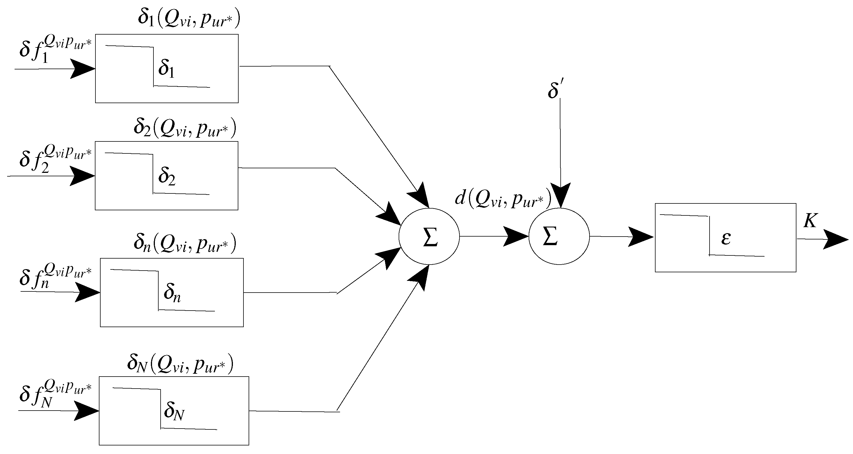
The FV functionality can be formulated as a distance metric as shown in Figure 1. Consider a prototype is selected to lock a cryptographic key K of a user u. During enrollment, each locking element locks a piece of information about the key K. During authentication, an unlocking element is extracted from the query sample , and is matched to all locking elements of the FV. The unlocking element can locate its corresponding locking element only if their similarity lies within a matching tolerance . Accordingly two corresponding locking and unlocking elements constitute a distance element:
where we define the operator ⌈⌉ as follows:
and
The accumulation of the individual distance elements constitutes the FV distance metric:
Considering the extra noise (chaff) errors , the total distance (matching error) between a query and its prototype should not exceed the FV error correction capacity . Accordingly, the proposed formulation of the FV functionality is:
where the distance is smaller than , this function outputs , which implies that the locked cryptographic key is released (that should occur for WC samples where ). Otherwise, the function outputs which implies that the key is not released (that should occur for BC samples where ).
To achieve the above condition, an effective distance metric learning approach is needed to optimize the FV distance metric (defined by Equation (4)), so that the WC and BC distance ranges are separated. In this case, the simple threshold rule (error correction capacity of the FV decoder) discriminates between genuine and impostor samples with high accuracy.
3. Related Work
The distance metric learning concept has been introduced mainly to enhance the performance of distance classifiers that take explicit distances (or kernels) as inputs, e.g., KNN, SVM, etc., [14]. For such distance/kernel-based classifiers, a distance function that measures the true proximity between feature representations (FR) of patterns is firstly designed, and is then fed to the classification stage. The performance of such classifiers relies on the quality of the employed distance measure, which in turn relies on the employed FR, the distance function applied to the representation, and the prototypes that are used as references for distance computations.
In the literature, such systems are optimized with the use of distance function learning [19], and/or prototype selection [20]. Distance function learning is done through the optimization of a parameterized function, so that the WC distances are minimized and BC distances are maximized. Examples of the employed distance functions are distance [21], Chi-squared [22], weighted similarity [23], and probability of belongingness to different classes [24]. However, most employed distance functions take the following form:
where and are the feature representations for the questioned and the prototype samples, respectively. This technique provides a means of translating hardly separable distributions to a space where the distributions are more separable. In order to having the conventional pattern recognition approaches hold in the new space, A is restricted to being a symmetric and positive definite matrix (or kernel), such that df(.) is a metric function [19]. According to Equation (6), it is obvious that entries of the A matrix determine the impact of the pairwise distances between individual features on the distance measure. Thus, learning A implies feature selection [25]. It has been shown that the accuracy of this metric increases when full matrices are considered (i.e., not only a diagonal matrix but some weighted relations among individual distances exist) [26].
Also, it is shown that global distance functions do not frequently represent all classes [27]. Instead, the concept of local distance functions is presented [19]. For instance, the metric tensor concept is represented, where instead of learning a metric A for the whole population, a specific metric is learned for every class T. This approach becomes complex for large numbers of classes, and some authors have suggested grouping similar classes under larger classes so that a trade-off between global and class-specific distance functions can be achieved [23]. Moreover, as indicated earlier, the quality of the proximity measure also depends on the prototype set used as a reference for distance measuring. Prototype selection has been extensively studied for distance-based classifiers like KNN [20].
4. Proposed Method
4.1. Overview
Since existing distance learning approaches are mainly designed for the enhanced performance of generic distance classifiers such as KNN, SVM, etc., there are no specific constraints applied to either classifier complexity, training size, or employed representation. Conversely, there are restrictions that apply when designing distance metrics for signature-based bio-cryptography. For instance, these systems involve a simple thresholding distance classifier which makes it hard to model complex problems like offline signature verification (OLSV). Moreover, OLSV systems should learn from limited positive signature samples and almost no forgeries are available during the design phase. Lastly, the design of such systems requires concise feature representations which might not capable of alleviating the high variability in the signature images. These design constraints require a specialized distance learning method for the problem at hand.
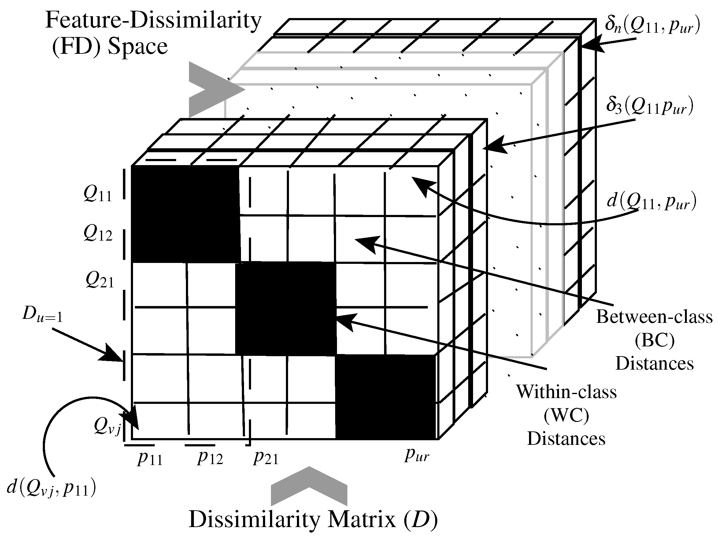
In this paper, the distance metric defined by Equation (4) is optimized based on a mixture of Feature-Distance (FD) space [28,29] and dissimilarity matrix analysis. Figure 2 illustrates the different distance metric computational spaces. Let us assume a system is designed for U different classes, where for any class u there are R prototypes (templates) . Also, a class v provides a set of J questioned samples . The distance between a questioned sample and a prototype is . The distances between all the questioned and prototypes samples constitute a dissimilarity matrix, where each row contains distances from a specific query to all of the prototypes.
Where questioned and prototype samples belong to the same class, i.e., , the distance sample is a WC sample (black cells in Figure 2). On the other hand, if questioned and prototype samples belong to different classes, i.e., , then the distance sample is a BC sample (white cells in Figure 2). An ideal distance metric implies that all the WC distances have zero values, while all the BC distances have large values. This occurs when the employed metric d absorbs all the WC variabilities, and detects all the BC similarities. The proposed approach aims to enlarge the separation between the BC and WC distance ranges, such that a simple distance threshold rule (like that involved in error correcting codes) produces accurate classification.
As shown in the figure, a distance measure accumulates some distance elements that are computed in the FD space, where the distance between a query and a prototype is measured by the distance between their feature representations and , respectively (see Equations (1)–(4)). To enlarge the separation between the WC and BC ranges, individual distance elements should be designed properly such that the WC instances will have low values and the BC instances high values. Since a distance element relies on a specific feature and its associated tolerance , these building blocks should be optimized accordingly.
In the case of signature-based bio-cryptography systems, the optimization of the aforementioned distance metric is a challenging task since a concise representation must be selected from high-dimensional representations, especially when only a few positive samples and almost no forgery samples are available for training. We tackle this challenging problem by proposing a hybrid Global-Local learning framework that also achieves a trade-off between global and local distance metric approaches [23]. The global learning process overrides the curse -of -dimensionality by using huge numbers of samples of a development dataset for learning in the original high-dimensional feature space. Therefore, it becomes feasible for the local learning process to learn in the resulting reduced space even when limited samples are available for training.
This section provides a detailed description of the proposed GLDM distance metric learning framework illustrated in Figure 3 (please note that all the algorithms proposed in this paper are listed in the Figure). In the first step, a large number of samples of a global dataset is used to design a global distance metric that differentiates between WC and BC samples of the population. a preliminary feature space of huge dimensionality M is produced and is reduced to a global space of dimensionality through the application of a Boosting Distance Elements (BDE) process. This BDE process runs in the Feature-Dissimilarity (FD) space resulting from the application of a dichotomy transformation, where distance elements are designed by selecting their constituting features and adjusting their tolerance values.
Then, once enrolling samples are available for a user, they are used to tune the global metric and produce a local (user-specific) distance metric. The local metric discriminates between the specific-class WC distances and the BC distances that are computed by comparing class samples to samples of other classes or forgeries. To this end, the local samples and some samples from the global dataset are represented in the global space of dimensionality . Additional dichotomy transformation and BDE processes run in the reduced space to produce a local space of dimensionality . Moreover, since different columns in the dissimilarity matrix might differ in accuracy (see Figure 2), we determine the best signature prototype by selecting the most stable and discriminant column.
Finally, depending on whether or not a local solution is available, either a global or a local distance metric is computed by employing Equations (1)–(4), using the distance element constituents produced by the above steps. It is important to note that for both global and local distance metric computations, only the best elements have been used since the metric produced is mainly designed for building FV systems that require a concise number of locking/unlocking elements.
4.2. Global Distance Metric Learning
Algorithm 1 describes the processing steps for learning global distance metric constituents. A feature representation of high dimensionality M is extracted from a global dataset G and is translated to the FD space by applying a dichotomy transformation. A boosting distance elements (BDE) process (Algorithm 2) runs in the FD space producing a set of global feature indexes and their associated tolerance values , where .
| Algorithm 1 Global Distance Metric Learning (GDM) |
Input: Global set consists of S samples from different classes.
|
| Algorithm 2 Boosting Distance Elements (BDE) |
Input: Training set , where , B is the number of boosting iterations, [[validation set is the early stopping parameter]].
|
4.2.1. Dichotomy Transformation
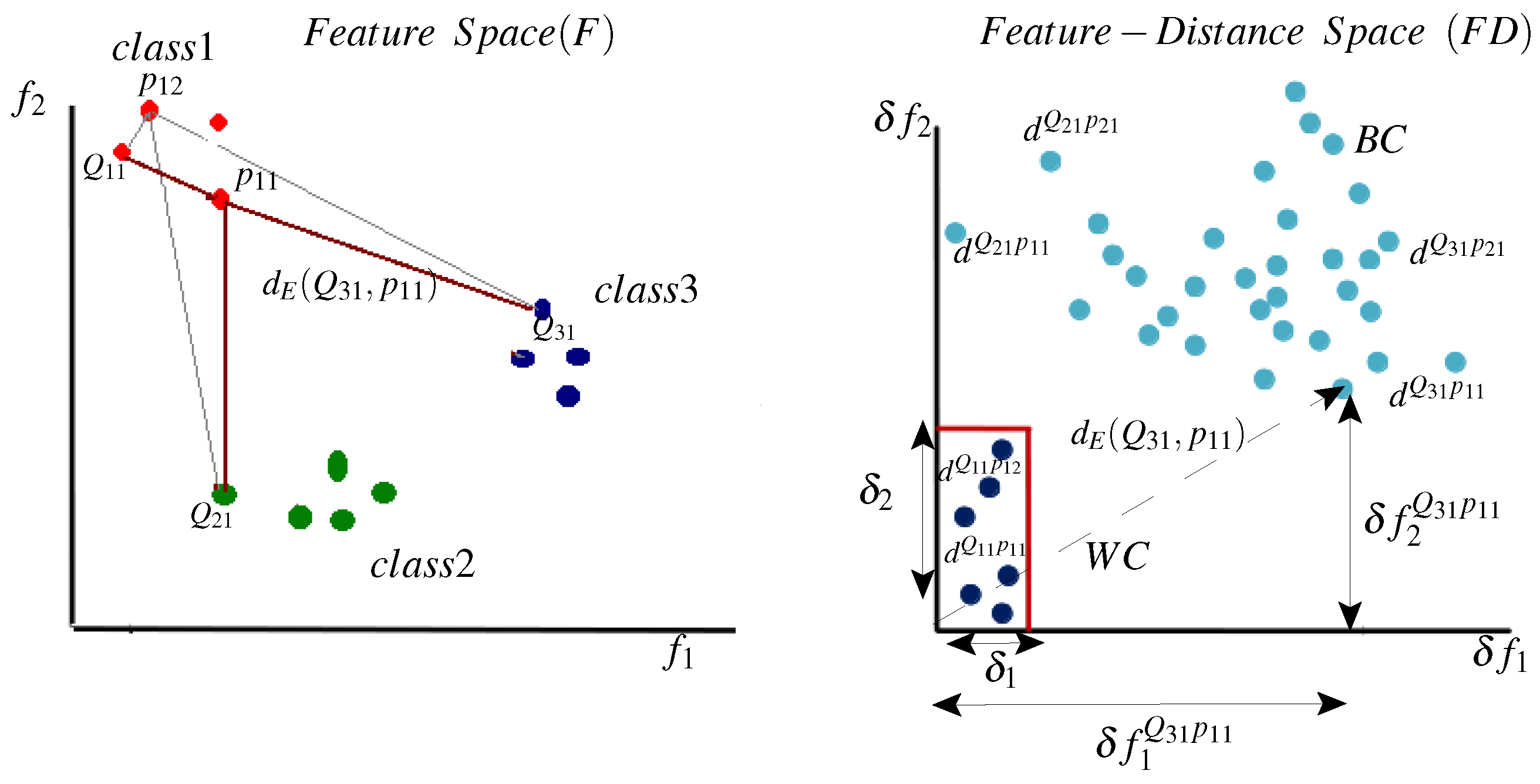
The dichotomy transformation is applied to the original feature space F and translates samples to the feature-distance space, where distance elements are selected and optimized. Each distance element is computed based on a single feature and its associated tolerance value . To illustrate the importance of this transformation, consider the example shown in Figure 4. On the left side, objects from three classes are represented in the feature space F. For simplicity, only two features and are shown in this figure, while typical representations might have high dimensionality. In this example, we assume that class 1 has two prototypes and . Also, let us consider, for now, that the employed distance function is the Euclidean distance:
It is clear that a distance metric that is built on top of this representation is discriminative. WC distances (like ) are generally smaller than BC distances (like ). However, in the feature space F, the impact of each feature on the WC and BC distances is not clear. With representations of high dimensionality, high number of classes, and a small number of training samples per class, it is not feasible to select the most discriminative features in the feature space F.
On the other hand, in the feature-distance space , the impact of every individual feature on the WC and BC distances is clear, (see right side of Figure 4). In this space, a distance is represented by the length of the distance vector , where:
is the absolute feature distance defined by Equation (3).
Accordingly, the impact of each distance element on the overall distance metric (defined by Equation (7)) is explicit in the FD space. Projecting the dissimilarity vector on different axes of the FD space, we can determine the discriminative power of each dimension. For instance, it is obvious that is more discriminative than . For all samples belonging to class 1, (like ), and for all other class samples (like and , . On the other hand, is less discriminant. For the class 2 query , , it is the same as with that for the class 1 query . Besides being easier to rank features in the space, the multi-class problem with few training samples per class in F space is transformed into a more tractable two-class problem in the new space, with more training samples per class. Moreover, in the new space, it is possible to learn a tolerance value , for each dimension , which discriminates between WC and BC distance instances. Embedding this tolerance information in computations of the distance metric transforms the Euclidean metric (defined by Equation (7)), which is sensitive to representation variabilities, into a more robust metric (defined by Equation (4)).
The aforementioned transformation method is applied for both global and local learning phases. For the global phase, the original representation of huge dimensionality M is projected to the FD space to be filtered by a Boosting Distance Elements (BDE) algorithm (Algorithm 2), producing a global space of reduced dimensionality . (see Section 4.3 for use in applying dichotomy transformation during local distance metric learning).
4.2.2. Boosting Distance Elements
Algorithm 2 describes the BDE process. Training distance samples are represented in the FD space of a dimensionality A and they are initially given equal weights (Step 1). They are then sent to a boosting feature selection (BFS) method [30], for fast searching in high dimensional spaces (Steps 2:20). At each boosting iteration b, the best dimension is selected, along with the adjustment of its associated tolerance that best splits the WC and BC distances (Steps 5:11). After each boosting iteration, training samples are given new weights based on the extend to which they are accurately classified by the current distance element, and the weight distribution is updated accordingly (Steps 12:13). Before proceeding to the next boosting iteration, the current committee of distance elements is considered as a distance metric, and is validated using a validation dataset, where the Area Under the Curve (AUC) is employed for performance validation (The validation step is employed only during the global learning step, where sufficient numbers of samples exist. On the other hand, only a training set is used during the local BDE process). Once the maximum number of boosting iterations B is reached, or a performance degradation is seen for the last validations, the process ends and produces a list of feature indexes and their associated tolerances of length (Steps 14:19).
This BDE process runs during both the global and local phases. In the global phase, the input is of dimensionality , and it produces a global representation of dimensionality . (see Section 4.3. for using BDE algorithm during local distance metric learning).
4.3. Local Distance Metric Learning (LDM)
This process runs for every individual class (user), for tuning the global metric to the specific user. Algorithm 3 describes the LDM process. The local set (containing R samples) and a subset of the global set (containing I samples) are represented in the global representation of dimensionality produced by above global learning process. Then, they are translated to a global FD space producing distance samples , which consist of WC and BC samples of same dimensionality . These samples are sent to another BDE process that runs in the resulting FD space (as described in Algorithm 2), and it produces a local space of dimensionality consisting of a set of local feature indexes and their associated tolerance values . The resulting local representation could be employed directly to compute a local distance metric using any available prototype as a reference; however, we propose a prototype selection process which instead picks the most stable and discriminant prototype for enhancing the accuracy of the metric.
Algorithm 4 illustrates the prototype selection process. Firstly, the global representations and of the local and global sets, respectively, are translated to the reduced local space by means of the local feature indexes (extracted in Step 6 of Algorithm 3). The produced local representations and are used to generate a dissimilarity matrix D. To that end, the local tolerance values (extracted in Step 6 of Algorithm 3) are used for the distance metric computations defined by Equations (1)–(4). The produced matrix D is then used to select the most stable and discriminant prototype .
| Algorithm 3 Local Distance Metric Learning (LDM) |
Input: Local set consists of R prototypes of local class, feature representation of global set G of dimensionality M (extracted in Algorithm 1), global feature indexes of dimensionality (output of Algorithm 1).
|
| Algorithm 4 Prototype Selection (PS) |
Input: Global feature representations and of dimensionality for global and local sets, respectively, local feature indexes , local feature tolerance .
|
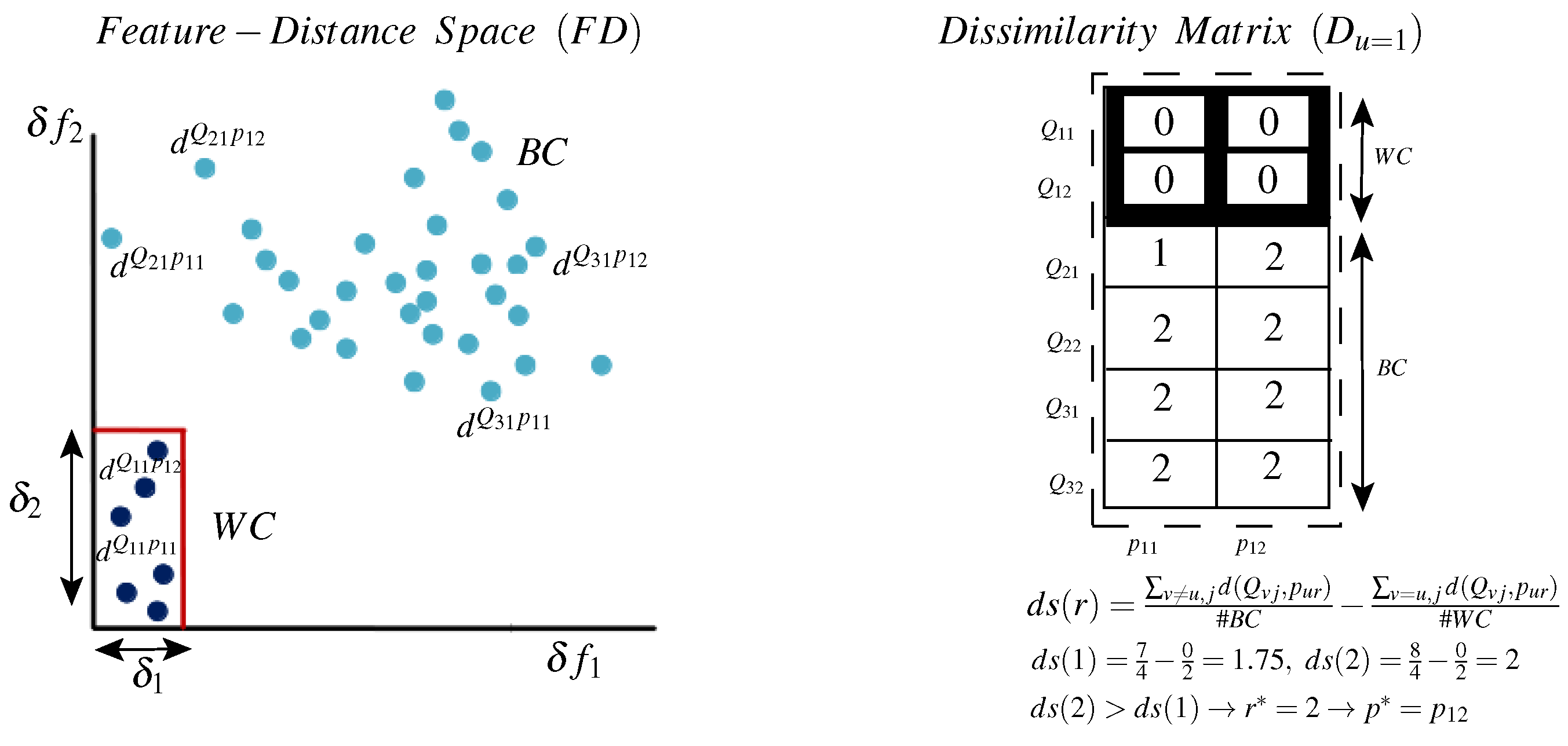
Figure 5 illustrates the prototype selection method by analyzing a dissimilarity matrix D and its relation to the representation space. On the left side, the WC and BC samples are represented in the space. It is obvious that different prototypes (different columns in the matrix D) produce different distance values, where significant variability exists for the WC and the BC classes. Moreover, in this space, it is not clear which prototype is the most informative. On the right side, distance samples are projected to a dissimilarity matrix , where each row contains distances between a specific query to all prototypes and each column contains distances between all queries to a specific prototype. Here, we investigate a part of D (see Figure 4) for a specific class . Further, for simplicity, only two prototypes are shown for class 1 ( and ), and few query samples have been used (two queries for the local class and and two queries for each of the global classes 2 and 3). However, practical matrices could have a high number of prototypes (columns) and a high number of queries (rows). Moreover, this illustrative matrix is generated based on two features only ( and ), i.e., , and so the distance values . Nevertheless, practical problems might include higher dimensionality. For instance, for the distance values .
It is clear that the dissimilarity matrix provides an easier way of ranking prototypes according to their discriminative power. For instance, for class 1, is more discriminative than because for all BC samples, whereas for , (because ). Thus, for this class, measuring the distance relative to results in more isolated WC and BC distance ranges.
To automate the dissimilarity matrix analysis and the selection of the best prototype, we propose a distance separability measure:
The left part of the above equation measures the discriminative power of a prototype where high values indicate a large separation between global and local samples (BC distances). The right side for its part measures the stability of a prototype in which low values indicate a small separation between local samples (WC distances). Accordingly, we select the prototype that maximizes this distance separability measure and the best prototype is given by:
5. Experimental Methodology
The experiments conducted investigate both the proposed GLDM distance metric learning approach and the signature-based FV bio-cryptosystem, designed based on the resulting distance metrics. First, the experimental databases are split into a global (development) set G and an exploitation set that consists of several local sets (L), one for each user. A preliminary feature representation (FR) of huge dimensionality M is extracted and used to generate a preliminary dissimilarity matrix. This matrix is refined several times by applying the different steps of the GLDM learning approach (as described by Figure 3). The importance of the different processing steps is measured by their impact on separating the WC and BC distance ranges. The learned distance metrics are then used to design the target signature-based FV system. Since we proposed the first bio-cryptosystem based on offline signature images, there is no benchmark available for testing our system, and we make comparison with state-of-the-art classical signature verification (SV) systems instead. However, we emphasis here that this comparative study might be biased because while the FV systems involve a very simple classification rule (a distance threshold) and employs concise feature representations, the SV systems might employ complex classification rules and high dimensional representations.
5.1. Databases
Two different offline signature databases have been used for proof-of-concept simulations: the Brazilian PUCPR database [17], and the GPDS-300 database [18]. Firstly, we executed a proof-of-concept for GDML prototyping using the PUCPR database, and then the concept is generalized by testing a GLDM-based FV system using both of the databases. While the PUCPR database is composed of random, simple and skilled forgeries, the GPDS database for its part is composed of random and skilled forgeries. Random forgeries occur when the query signature presented to the system is mislabeled to another user. Further, forgers produce random forgeries when they know neither the signer’s name nor the signature morphology. For simple forgeries, the forger knows the writer’s name but not the signature morphology, and can only produce a simple forgery using his writing style. Finally, skilled forgeries imitate the signatures as they have access to a genuine signatures sample.
5.1.1. Brazilian PUCPR Database
The PUCPR database contains 7920 samples of signatures that were digitized as 8-bit grayscale images over 400X1000 pixels at a resolution of 300 dpi. The signatures were provided by 168 of these writers. For the last 108 writers, there are only 40 genuine signatures per writer, and no forgeries. We consider these signatures as the global dataset (G), and they are employed for the GDM learning phase. For the first 60 writers, there are 40 genuine signatures, 10 simple forgeries and 10 skilled forgeries per writer. These signatures are considered as the exploitation dataset consisting of several local subsets (L), one per user. Of these, the first 30 genuine signatures have been used for the LDM learning phase; however, the last 10 genuine signatures and all of the different forgeries have been used for performance evaluation.
5.1.2. GPDS-300 Database
The GPDS-300 database contains signatures of 300 users, which were digitized as 8-bit grayscale images at a resolution of 300 dpi. This database contains images of different sizes (varying from to pixels). All users have 24 genuine signatures and 30 skilled forgeries. The database is split into two parts. One part contains the signatures of the last 140 users and is considered as the global set (G) used for GDM training. The other part contains the signatures of the first 160 users and is considered as the exploitation dataset that consists of several local subsets (L), one per user; as well. Of these, the first 14 genuine signatures have been used for the LDM learning phase; however, the last 10 genuine signatures and all of the forgeries have been used for performance evaluation.
5.2. Global Distance Metric Learning
The processing steps of the GDM learning algorithm (Algorithm 1) are executed using the global dataset (G) of both databases as follows:
5.2.1. Feature Extraction
The Extended-Shadow-Code (ESC) [31] and Directional Probability Density Function (DPDF) [32] are employed. Features are extracted based on different grid scales, hence a range of details are detected in the signature image. A set of 30 grid scales is used for each feature type, producing 60 different single scale feature representations. These representations are then fused to produce a FR of huge dimensionality, 30,201 [29].
5.2.2. Dichotomy Transformation
The initial dissimilarity matrix, is constituted by translating the FR, of M dimensionality, for all users of G, to a FD space of same dimensionality. As this matrix is huge, not all of its cells are used for the GDM learning process. Also, to avoid overfitting the G dataset, some of the WC and BC samples have been used for training, while other sets of samples have been used for validation.
5.2.3. Boosted Global Distance Elements
The BDE process (Algorithm 2) runs using the G learning sets. The number of boosting iterations B is set to 1000 and the early stopping parameter is set to 100. The input dimensionality 30,201. For the PUCPR database, the resulting dimensionality , while for the GPDS-300 database . The global distance metric is then computed using the resulting representation and the associated tolerance values according to Equations (1)–(4).
5.3. Local Distance Metric Learning
The processing steps of the LDM learning algorithm (Algorithm 3) are executed using the local dataset (L) of both databases as follows:
5.3.1. Feature Extraction and Filtering
Feature representations and of high dimensionality 30,201 are extracted from the local dataset L of each user and from a subset of the global dataset, which represent negative samples, respectively. Then, this original representation is filtered by , producing global representations and of the global and local training sets, respectively. The dimensionality of the resulting representation is for the PUCPR database and for the GPDS database.
5.3.2. Dichotomy Transformation
The dissimilarity matrix, is constituted by translating the global representations and to a FD space of same dimensionality . As this matrix is huge, not all of its cells have been used for the LDM learning process.
5.3.3. Boosted Local Distance Elements
The BDE process (Algorithm 2) runs using the learning samples. The number of boosting iterations B is set to 100 and no early stopping is applied. The input dimensionality are for the PUCPR database and for the GPD-300 database. The local distance metric is then computed using the resulting feature indexes and the associated tolerance values according to Equation (4), where only the first indexes are used. The dissimilarity cells are re-computed based on this local metric, and produce a dissimilarity matrix.
5.3.4. Prototype Selection
5.4. Fuzzy Vault Encoding and Decoding
Once the local distance metric is learned, the information embedded in its constituting distance elements is used for FV encoding and decoding (as described in Section 2). In the encoding phase, we set the encoding message length and the cryptographic key K size to 128-bits. Accordingly, the distance metric constituents are extracted from the best enrolled signature prototype , and are quantized in 8-bit words. Then, the cryptographic key K is used to generate a polynomial of degree and the quantized features are then projected on the polynomial. The features and their projections constitute a set of genuine FV locking points. Finally, a set of chaff (noise) points are generated to conceal the genuine points, and both sets constitute the FV (For more details on how FV encoding/decoding works, see [6,16]).
During FV decoding, the same features are extracted from the query signature image Q. The features are quantized and matched with the FV points. Since the distance metric is designed such that WC distances are small and the BC distances are large, it is expected that most of decoding features of genuine query samples will match the FV locking points, while only a few features of impostor queries will match FV points. The matching points are then corrected by the FV error correction decoder, where we set the error correction capacity , and they are used to re-generate the polynomial and release the cryptographic key K to the user.
5.5. Performance Evaluation
5.5.1. Evaluation of the GLDM Approach
The proposed GLDM approach is evaluated by investigating its power to generate well separated WC and BC distance ranges. A testing distance matrix is generated for each user of local datasets.
To investigate the different processing steps of the proposed approach, the impacts of the different learning steps on the separation of the WC and BC clusters are decoupled by employing the following experimental scenarios:
- Random distance metric (RDM): features are randomly selected from the M feature extractions, and are used to produce a random distance metric.
- Global distance metric (GDM): the global metric is used for distance computations. This setting investigates the extend to which a global metric generalizes to unseen classes/users.
- Strict local distance metric (SLDM): a modified version of the local metric is used for distance computations, where the learned feature tolerance is not employed. We can thus decouple the impact of embedding the modeled feature tolerance in the metric computations, and only test the applicability of tuning the global metric to specific classes/users. In all the above scenarios, we employed a strict distance metric as a non-tolerant variant of distance metrics, where the distance element (defined by Equation (1)) is replaced by a strict distance element:
For all the above cases, the testing datasets are used to generate dissimilarity matrices, according to the investigated scenario. The separability of the WC and BC clusters are then measured by the Hellinger distance [33]. Assuming normal distributions of the WC and BC clusters, the squared Hellinger distance between them is given by:
where , and , are the mean and variance values for and distances for a specific user u, respectively.
To measure the cluster separability for the different types of forgery, we compute , and , with the parameters and of the BC cluster are computed each time, based on the distances from samples of a specific type of forgeries. Also, we report , where the distribution parameters are computed according to distance measures of all forgery types. For all cases, these measures are averaged over all U users:
Moreover, since the main target application of the proposed GLDM approach is the development of a reliable FV system, we decouple here any factor that impacts the recognition accuracy of such a system other than those related to the GDLM method. More specifically, FV recognition accuracy relies on the separability of the WC and BC distance ranges (which reflects the effectiveness of the GLDM approach), as well as on the error correction capacity (which is equivalent to the distance threshold that split the WC and BC ranges (see Equation (5)). Accordingly, we decouple the impact of the choice of the threshold and only test the impact of the metric on FV performance. To that end, we generate ROC (receiver operating curve) curves by computing recognition errors for all possible distance measures. A ROC curve plots the False Accept Rate (FAR) against the Genuine Accept Rate (GAR) for all possible thresholds (all distance measures). FAR for a specific threshold is the ratio of forgery samples with a distance measure smaller than this threshold. GAR is the ratio of genuine samples with a distance measure smaller than the threshold. In order to have a global assessment of the FV quality, we compute and average the AUC (area under ROC curves), for all users in the testing subset. A high AUC indicates more separation between the distance score distributions for the WC and BC classes.
5.5.2. Evaluation of the GLDM-Based FV System
After evaluating the GLDM approach, we investigate the performance of the FV bio-cryptosystem, designed based on the learned distance metrics, by employing the same experimental scenarios mentioned above. To measure actual recognition rates, we apply a fixed FV error correction capacity , where this value is empirically selected to compensate between the FRR and FAR errors (For a key size of 128-bits, the polynomial degree is and the corresponding error correction capacity is . A trade-off between accuracy and security could be achieved by changing the key size (and the error correction capacity accordingly)). Then, we report the average error rate (), where
The False Reject Rate () is the ratio of rejected genuine queries; , and are ratios of accepted random, simple, and skilled forgeries, respectively.
6. Results and Discussion
6.1. Results of the GLDM Approach
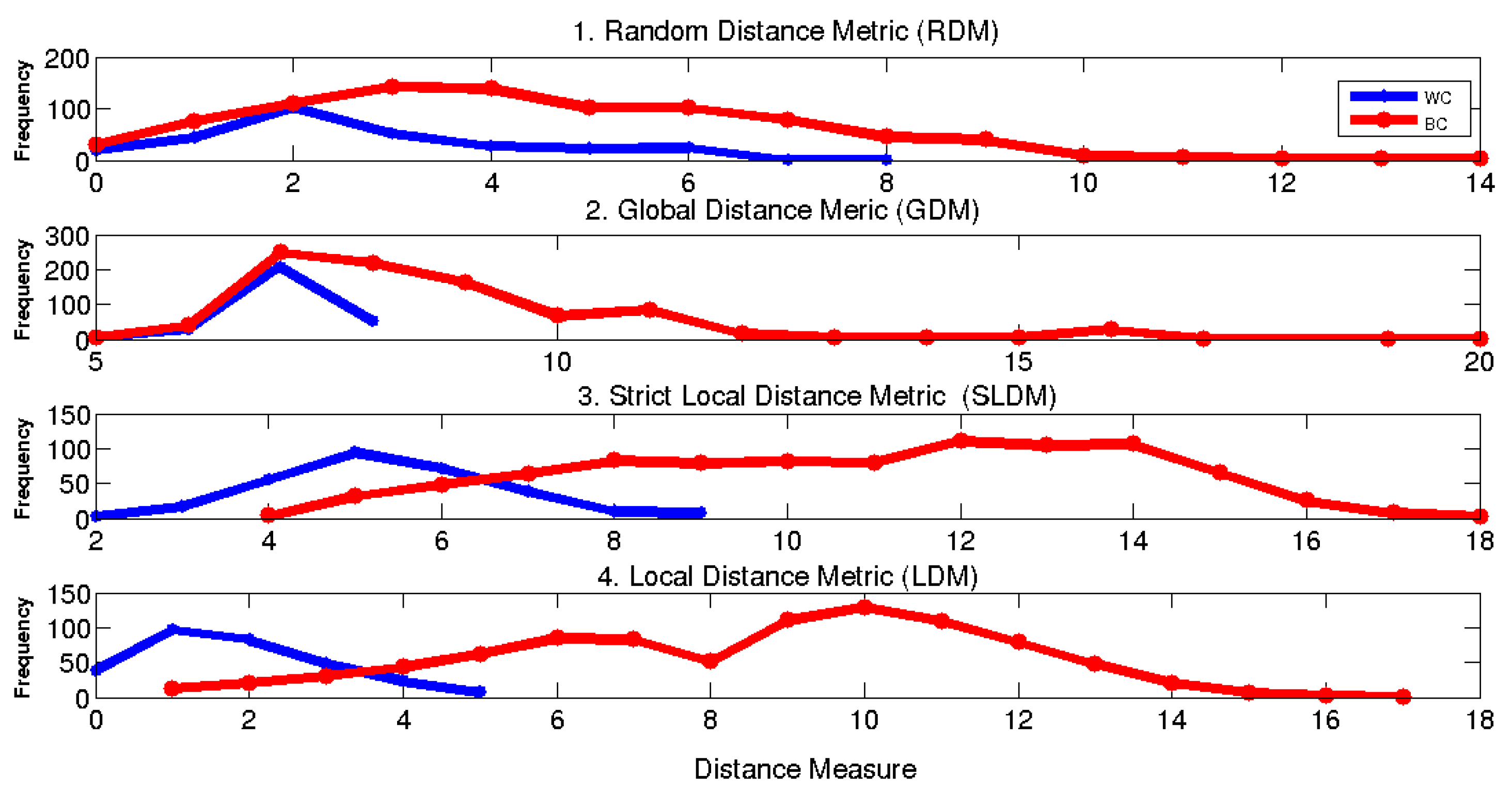
Figure 6 illustrates the impact of each processing step on the separation of the WC and BC clusters, for a specific user. It is obvious that, without distance metric learning, the distance distributions are overlapped. Learning a global metric using a global dataset increases the separation. This validates our hypothesis that distance metrics learned based on high dimensional FRs extracted from large numbers of classes, relatively, generalize for unseen classes. Running a local metric learning process using class-specific datasets increased separability. This validates our hypothesis that, the global metrics are adaptable for new classes. Embedding information about feature variability in distance metric computations increased the stability of the genuine class: for instance, the maximum distance score for the genuine class decreased from 9 to 5. This validates our hypothesis that the modeling of representation variability in the FD space absorbs some intrinsic signal variability.
Table 1 shows the average performance, where the Hellinger distance is averaged over all users and for the different types of forgeries. It is obvious that each processing step increased the distances between the WC and BC distance distributions, for all types of forgeries. The average distance of all forgery distributions is increased from 0.24 to 0.66. Also, the average AUC is increased by about 47% (from 0.65 to 0.97).
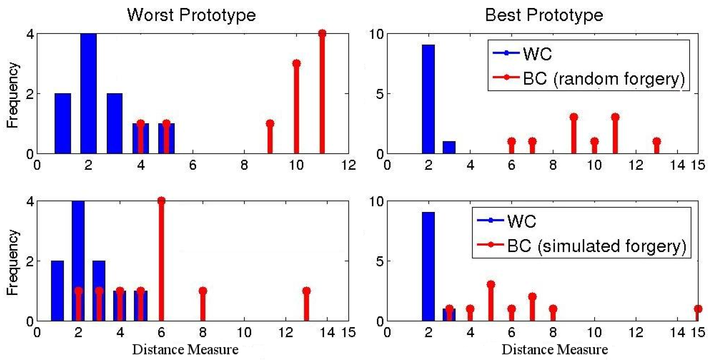
The distance measures reported above are averaged for all prototypes. However, class separation differs for the different prototypes. For instance, Figure 7 shows distributions of the best and worst prototypes for a specific user. For the worst prototype, a distance threshold results in , and . For the best prototype, , and .
6.2. Results of the GLDM-based FV System
Recognition rates for the FV system, designed based on the learned local distance metric , are reported in Table 2 and Table 3 for the PUCPR and GPDS databases, respectively. For the PUCPR database (see Table 2), it is clear that each step of the GLDM learning approach enhances the FV recognition performance and this result is correlated with the distance separability investigations reported in Table 1. Also, applying the prototype selection method (variant 5) enhances the FV performance significantly. The recognition rates of this FV variant (where all GLDM processing steps are executed) is compared to state-of-the-art classical signature verification (SV) systems.
The first three SV systems are writer-independent (WI-SV), where a global development (independent) database is used to generate a global classifier. All systems employed an ensemble technique such that the classification decision relies on multiple prototypes, and high dimensional presentations are employed. The other SV systems are writer-dependent (WD-SV), where one local (dependent) dataset is used to generate a local classifier per user. For these systems, various complicated techniques, such as the dynamic selection of classifier and ensemble methods, are employed for enhanced recognition.
Generally, although the proposed FV implementation can be considered a very simple classifier (only a distance threshold) with concise feature representations (only 20 features), its recognition rates are comparable to those of more complex SV systems. For instance, compared to state-of-the-art WI-SV systems (system 3), where both the FV and SV systems rely on a single prototype for authentication, the proposed FV bio-cryptosystem has shown similar accuracy, while employing only 20 features instead of the 555 features present in the SV system [29]. Thus, applying our proposed GLDM learning approach maintained the performance, while decreasing the representation complexity by about 96% (from 555 to only 20 features). Moreover, digitizing the feature values (as they are represented in 8-bit words for bio-cryptographic encoding), had no impact on the recognition accuracy. Recently, the authors proposed a hybrid WI-WD SV system that tunes a global representation to specific users (see system 7). This system outperforms the aforementioned SV systems and provides similar insights about the effectiveness of applying a hybrid Global-Local training scheme.
For the GPDS database (see Table 3), each step of the GLDM learning approach enhances the FV recognition performance, providing results similar to the PUCPR experimental results. Comparisons with state-of-the art SV systems are promising as well. The first SV system employed a WI-SV classifier, where skilled forgery samples are used to train the global classifier. The following four SV systems employed WD-SV classifiers. The first three WD-SV systems also used skilled forgery samples to train the classifiers. This might bias the performance evaluation process since such knowledge is not available for training practical SV systems, e.g., banking systems. On the other hand, for the last WD-SV system, no forgery knowledge is used for training; however, complicated classification rules, such as the dynamic selection of classifiers and ensemble methods are employed for enhanced recognition. The hybrid WI-WD SV system outperforms both pure WI and WD systems, which leads to a similar conclusion as with the PUCPR database experiments, and supports the hypothesis regarding the effectiveness of tuning global solutions to specific classes. The proposed FV system has shown performance that are comparable to those of such complicated SV systems, where no forgery samples are used for training, proving the effectiveness of the proposed GLDM learning approach and supporting the proposed approach in modeling FV systems as distance metrics.
7. Conclusions
This paper proposed an approach for learning distance metrics adapted for bio-cryptosystem design. The proposed approach produces global metrics that generalize well to unknown classes that are not used for training. In addition, these metrics can be further tuned to new classes. This property permits the design of global classification systems adaptable to specific classes. Moreover, the produced metrics rely on concise representations, in terms of number of employed feature extractions and prototypes. This allow the design of systems with limitations in their computational complexity and that rely on high-dimensional feature representations, such as signature-based bio-cryptosystems. In addition, the modeling of representation variability and the selection of discriminant prototypes enhance the distance metric efficiency.
The proposed Global-Local distance metric (GLDM) learning approach is applied to the design of a key binding bio-cryptosystem based on the fuzzy vault (FV) scheme and handwritten signature images. To that end, the FV system functionality is formulated as a simple thresholding distance classifier. It is shown that such a simple classifier provides a level of accuracy that is as high as that of complex signature verification (SV) systems in the literature.
The proposed approach can also be employed as an intermediate tool for designing traditional feature-based classifiers, where the produced distance metrics feed distance-based classifiers, e.g., KNN. Future work will investigate the power of the proposed approach on other applications (e.g., face recognition, video surveillance, image retrieval, etc.). Also, comparing the effectiveness of the produced metrics to that of other local distance design methods in the literature is of great interest.
Acknowledgments
This work was supported by the Natural Sciences and Engineering Research Council of Canada and BancTec Inc., Montreal, QC, Canada.
Author Contributions
G.E., R.S. and E.G. conceived and designed the experiments; G.E. performed the experiments; G.E., R.S analyzed the data; G.E., R.S. and E.G. wrote the paper.
Conflicts of Interest
The authors declare no conflict of interest.
References
- Jain, A.K.; Ross, A.; Pankanti, S. Biometrics: A Tool for Information Security. IEEE Trans. Inf. Forensics Secur. 2006, 1, 125–143. [Google Scholar] [CrossRef]
- Uludag, U.; Pankanti, S.; Prabhakar, S.; Jain, A.K. Biometric Cryptosystems: Issues and Challenges. Proc. IEEE 2004, 92, 948–960. [Google Scholar] [CrossRef]
- Soutar, C.; Roberge, D.; Stojanov, S.A.; Gilroy, R.; Vijaya Kumar, B.V.K. Biometric Encryption Using Image Processing construction. SPIE 1998, 3314, 178–188. [Google Scholar]
- Davida, G.I.; Frankel, Y.; Matt, B.J. On enabling secure applications through off-line biometric identification. In Proceedings of the 1998 IEEE Symposium on Security and Privacy, Oakland, CA, USA, 6 May 1998; pp. 148–157. [Google Scholar]
- Davida, G.I.; Frankel, Y.; Matt, B.J.; Peralta, R. On the relation of error correction and cryptography to an offline biometric based identification scheme. In Proceedings of the Workshop Coding and Cryptography, Paris, France, 11–14 January 1999; pp. 129–138. [Google Scholar]
- Juels, A.; Wattenberg, M. A fuzzy commitment scheme. In Proceedings of the 6th ACM Conference on Computer and Communications Security, Singapore, 1–4 November 1999; pp. 28–36. [Google Scholar]
- Juels, A.; Sudan, M. A fuzzy vault scheme. In Proceedings of the 2002 IEEE International Symposium on Information Theory, Lausanne, Switzerland, 30 June–5 July 2002; p. 408. [Google Scholar]
- Nandakumar, K.; Jain, A.K.; Pankanti, S. Fingerprint-Based fuzzy vault: implementation and performance. IEEE Trans. Inf. Forensic Secur. 2007, 2, 744–757. [Google Scholar] [CrossRef]
- Lee, Y.J.; Park, K.R.; Lee, S.J.; Bae, K.; Kim, J. A new method for generating an invariant iris private key based on the Fuzzy Vault system. IEEE Trans. Syst. Man Cybern. Part B Cybern. 2008, 38, 1302–1313. [Google Scholar]
- Meenakshi, V.S.; Padmavathi, G. Retina and Iris based multimodal biometric Fuzzy Vault. Int. J. Comput. Appl. 2010, 1, 67–73. [Google Scholar] [CrossRef]
- Wang, Y.; Plataniotis, K.N. Fuzzy vault for face based cryptographic key generation. In Proceedings of the Biometrics Symposium, Baltimore, MD, USA, 11–13 September 2007; pp. 1–6. [Google Scholar]
- Impedovo, D.; Pirlo, G. Automatic Signature Verification: the State of the Art. IEEE Trans. Syst. Man Cybern. Part C Appl. Rev. 2008, 38, 609–635. [Google Scholar] [CrossRef]
- Freire-Santos, M.; Fierrez-Aguilar, J.; Martinez-Diaz, M.; Ortega-Garcia, J. On the applicability of off-line signatures to the Fuzzy Vault construction. In Proceedings of the Ninth International Conference on Document Analysis and Recognition, Parana, Brazil, 23–26 September 2007. [Google Scholar]
- Yang, L. Distance Metric Learning: A Comprehensive Survey; Michigan State University: East Lansing, MI, USA, 2006. [Google Scholar]
- Eskander, G.S.; Sabourin, R.; Granger, E. On the dissimilarity representation and prototype selection for signature-based bio-cryptographic systems. Similarity-Based Pattern Anal. Recognit. 2013, 7953, 265–280. [Google Scholar]
- Eskander, G.S.; Sabourin, R.; Granger, E. Bio-Cryptographic system based on offline signature images. Inf. Sci. 2014, 259, 170–191. [Google Scholar] [CrossRef]
- Freitas, C.; Morita, M.; Oliveira, L.; Justino, E.; Yacoubi, A.; Lethelier, E.; Bortolozzi, F.; Sabourin, R. Bases de dados de cheques bancarios brasileiros. In Proceedings of the XXVI Conferencia Latinoamericana de Informatica, Atizapan de Zaragosa, Mexico, 18–22 September 2000. [Google Scholar]
- Vargas, J.; Ferrer, M.; Travieso, C.; Alonso, J. Off-line handwritten signature GPDS-960 corpus. In Proceedings of the Ninth International Conference on Document Analysis and Recognition, Parana, Brazil, 23–26 September 2007; pp. 764–768. [Google Scholar]
- Ramanan, D.; Baker, S. Local Distance Functions: A Taxonomy, New Algorithms, and an Evaluation. IEEE Trans. Pattern Anal. Mach. Intell. 2011, 33, 794–806. [Google Scholar] [CrossRef] [PubMed]
- Garcia, S.; Derrac, J.; Cano, J.R.; Herrera, F. Prototype Selection for Nearest Neighbor Classification: Taxonomy and Empirical Study. IEEE Trans. Pattern Anal. Mach. Intell. 2012, 34, 417–435. [Google Scholar] [CrossRef] [PubMed]
- Frome, A.; Singer, Y.; Malik, J. Image retrieval and classification using local distance functions. Adv. Neural Inf. Process. Syst. 2007, 19, 417–424. [Google Scholar]
- Domeniconi, C.; Peng, J.; Gunopulos, D. Locally adaptive metric nearest-neighbor classification. IEEE Trans. Pattern Anal. Mach. Intell. 2002, 24, 1281–1285. [Google Scholar] [CrossRef]
- Babenko, B.; Branson, S.; Belongie, S. Similarity metrics for categorization: From monolithic to category specific. In Proceedings of the 2009 IEEE 12th International Conference on Computer Vision, Kyoto, Japan, 29 September–2 October 2009. [Google Scholar]
- Mahamud, S.; Hebert, M. The optimal distance measure for object detection. In Proceedings of the 2003 IEEE Computer Society Conference on Computer Vision and Pattern Recognition, Madison, WI, USA, 18–20 June 2003. [Google Scholar]
- Guyon, I.; Elisseeff, A. An introduction to variable and feature selection. J. Mach. Learn. Res. 2003, 3, 1157–1182. [Google Scholar]
- Bar-Hillel, A.; Hertz, T.; Shental, N.; Weinshall, D. Learning and Mahalanobis metric from equivalence constraints. J. Mach. Learn. Res. 2005, 6, 937–965. [Google Scholar]
- Weinbeger, K.; Saul, L. Distance metric learning for large margin nearest neighbor classification. J. Mach. Learn. Res. 2009, 10, 207–244. [Google Scholar]
- Srihari, S.; Xu, A.; Kalera, M.K. Learning strategies and classification methods for Off-Line signature verification. In Proceedings of the Ninth International Workshop on Frontiers in Handwriting Recognition, Tokyo, Japan, 26–29 October 2004; pp. 161–166. [Google Scholar]
- Rivard, D.; Granger, E.; Sabourin, R. Multi-Feature extraction and selection in writer-independent offline signature verification. Int. J. Doc. Anal. Recognit. 2013, 16, 83–103. [Google Scholar] [CrossRef]
- Tieu, K.; Viola, P. Boosting image retrieval. Int. J. Comput. Vis. 2004, 56, 17–36. [Google Scholar] [CrossRef]
- Sabourin, R.; Genest, G. An Extended-Shadow-Code based approach for off-line signature verification. In Proceedings of the 12th IAPR International Conference on Pattern Recognition, Jerusalem, Israel, 9–13 October 1994; Volume 2, pp. 450–453. [Google Scholar]
- Drouhard, J.; Sabourin, R.; Godbout, M. A neural network approach to off-line signature verification using directional PDF. Pattern Recognit. 1996, 29, 415–424. [Google Scholar] [CrossRef]
- Cha, S.-H. Comprehensive survey on distance/similarity measures between probability density functions. Int. J. Math. Models Methods Appl. Sci. 2007, 1, 300–307. [Google Scholar]
- Santos, C.; Justino, E.; Bortolozzi, F.; Sabourin, R. An off-line signature verification method based on document questioned experts approach and a neural network classifier. In Proceedings of the Ninth International Workshop on Frontiers in Handwriting Recognition, Tokyo, Japan, 26–29 October 2004; pp. 498–502. [Google Scholar]
- Bertolini, D.; Oliveira, L.; Justino, E.; Sabourin, R. Reducing forgeries in writer-independent off-line signature verification through ensemble of classifiers. Pattern Recognit. 2010, 43, 387–396. [Google Scholar] [CrossRef]
- Justino, E.; Bortolozzi, F.; Sabourin, R. Off-line signature verification using HMM for random, simple and skilled forgeries. In Proceedings of the Sixth International Conference on Document Analysis and Recognition, Seattle, WA, USA, 3 September 2001; pp. 1031–1034. [Google Scholar]
- Batista, L.; Granger, E.; Sabourin, R. Applying Dissimilarity Representation to Off-Line Signature Verification. In Proceedings of the 2010 20th International Conference on Pattern Recognition (ICPR), Istanbul, Turkey, 23–26 August 2010; pp. 1293–1297. [Google Scholar]
- Batista, L.; Granger, E.; Sabourin, R. Dynamic Selection of Generative-Discriminative Ensembles for Off-Line Signature Verification. Pattern Recognit. 2012, 45, 1326–1340. [Google Scholar] [CrossRef]
- Eskander, G.; Sabourin, R.; Granger, E. Hybrid Writer-Independent–Writer-Dependent Offline Signature Verification System. IET Biom. J. Spec. Issue Handwrit. Biom. 2013, 2, 169–181. [Google Scholar] [CrossRef]
- Kumar, R.; Sharma, J.; Chanda, B. Writer-independent off-line signature verification using surroundedness feature. Pattern Recognit. Lett. 2012, 33, 301–308. [Google Scholar] [CrossRef]
- Ferrer, M.A.; Alonso, J.B.; Travieso, C.M. Offline Geometric Parameters for Automatic Signature Verification Using Fixed-Point Arithmetic. IEEE Trans. Pattern Anal. Mach. Intell. 2005, 27, 993–997. [Google Scholar] [CrossRef] [PubMed]
- Solar, J.R.; Devia, C.; Loncomilla, P.; Concha, F. Off-line Signature Verification using Local Interest Points and Descriptors. Lect. Notes Comput. Sci. 2008, 5197, 22–29. [Google Scholar]
- Ribeiro, B.; Gonçalves, I.; Santos, S.; Kovacec, A. Deep Learning Networks for Off-Line Handwritten Signature Recognition. Lect. Notes Comput. Sci. 2011, 7042, 523–532. [Google Scholar]
Figure 1.
Proposed formulation of the FV functionality as distance metrics: each unlocking element is matched against all locking elements , where it succeeds in locating the corresponding element only if the elements’ dissimilarity is within the modeled tolerance . To correctly decode the FV, and release the locked crypto-key K, the overall distance between the locking and unlocking messages , besides the noise error (resulting from false matching with chaffs), should not exceed the error correction capacity of the decoder.

Figure 2.
Illustration of computing distance metrics based on the feature distance (FD) and dissimilarity matrix representations: black and white cells represent WC and BC distances, respectively. The third dimension represents the Feature-Distance (FD) space. The distances between prototype and query samples constitute distance cells, which accumulates distance elements computed in the FD space. The distance cells constitute a dissimilarity matrix, where each row contains the distances from a specific query to all of the prototypes.

Figure 3.
A framework of the Global-Local Distance Metric (GLDM) learning approach: a global distance metric is designed with a generic dataset and thus applies to any class (user). Once enrolling samples are available for a specific class (user), they are used to tune the global metric and produce a local metric.

Figure 4.
Illustration of the transformation from original feature space F (left) to the feature-distance space (right) by applying dichotomy transformation. The distance between two samples in the F space is translated to a vector in the space, where each dimension represents the distance as measured by a single feature. Three classes are represented in F space (class 1: red, class 2: green and class 3: black). These three classes are transformed to two classes in space (WC: black and BC: blue). In the FD space, it is easier to rank distance elements by their impact on the enlargement of the separation between WC and BC distance ranges. Also, in space, it is easier to learn a tolerance value for each element that discriminates between WC and BC samples.

Figure 5.
Illustration of the transformation from the feature-distance (FD) space (left) to the dissimilarity Matrix D (right). All distance samples that are measured with reference to a specific prototype in the FD space (WC samples: black and BC samples: blue), are represented as a single column in the matrix D. Although, selection of best prototype is not clear in the space, simple analysis of the dissimilarity matrix locates the most stable and discriminant column which in turn determines the best prototype.

Figure 6.
Distance measure distribution for a specific user from the PUCPR database.

Figure 7.
Distance measure distributions for different prototypes for a specific user in the UPCR database.
Figure 7.
Distance measure distributions for different prototypes for a specific user in the UPCR database.


Table 1.
Average Hellinger distance over all users of the UPCR database for the different design scenarios.
Table 1.
Average Hellinger distance over all users of the UPCR database for the different design scenarios.
| Variant | ||||
|---|---|---|---|---|
| 0.29 | 0.60 | 0.66 | 0.73 | |
| 0.25 | 0.55 | 0.60 | 0.69 | |
| 0.14 | 0.43 | 0.47 | 0.59 | |
| 0.24 | 0.55 | 0.59 | 0.66 | |
| 0.65 | 0.77 | 0.93 | 0.97 |
Table 2.
Overall error rates (%) provided by systems designed by the PUCPR database.
| Application | Approach | Reference/Variant | # Prototypes | FRR | FAR | AER | ||
|---|---|---|---|---|---|---|---|---|
| Random | Simple | Skilled | ||||||
| SV | WI | 1. Santos [34] | 5 | 10.33 | 4.41 | 1.67 | 15.67 | 8.02 |
| 2. Bertolini [35] | 15 | 11.32 | 4.32 | 3.00 | 6.48 | 6.28 | ||
| 3. Rivard [29] | 1 | 13.53 | 0.12 | 0.43 | 14.95 | 7.26 | ||
| 15 | 9.77 | 0.02 | 0.32 | 10.65 | 5.19 | |||
| WD | 4. Justino [36] | - | 2.17 | 1.23 | 3.17 | 36.57 | 7.87 | |
| 5. Batista [37] | 9.83 | 0.00 | 1.00 | 20.33 | 7.79 | |||
| 6. Batista [38] | 7.50 | 0.33 | 0.50 | 13.50 | 5.46 | |||
| WI-WD | 7. Eskander [39] | 7.83 | 0.01 | 0.17 | 13.50 | 5.38 | ||
| FV | Proposed | 1. | 1 | 14.57 | 73.59 | 72.00 | 76.74 | 59.23 |
| 2. | 36.72 | 7.13 | 9.26 | 22.02 | 43.47 | |||
| 3. | 28.00 | 2.00 | 3.00 | 22.00 | 13.75 | |||
| 4. | 11.35 | 2.05 | 2.39 | 24.38 | 10.08 | |||
| 5. | 4.83 | 0.6 | 1.5 | 22.33 | 7.32 | |||
Table 3.
Overall error rates (%) provided by systems designed by the GPDS database.
| Application | Approach | Reference/Variant | Using Forgeries In Training | FRR | FAR | AER | ||
|---|---|---|---|---|---|---|---|---|
| Random | Skilled | Avg | ||||||
| SV | WI | 1. Kumar [40] | YES | 13.76 | – | 13.76 | – | 13.76 |
| WD | 2. Ferrer [41] | 14.10 | – | 12.60 | – | 13.35 | ||
| 3. Solar [42] | 16.40 | – | – | 14.20 | 15.30 | |||
| 4. Ribeiro [43] | 20.25 | – | – | 14.67 | 17.46 | |||
| 5. Batista [38] | NO | 16.81 | – | 16.88 | – | 16.84 | ||
| WI-WD | 6. Eskander [39] | 18.06 | 0 | 22.71 | - | 13.96 | ||
| FV | Proposed | 1. | NO | 23.50 | 70.07 | 72.02 | - | 55.19 |
| 2. | 48.31 | 13.60 | 45.17 | - | 35.69 | |||
| 3. | 39.00 | 3.19 | 16.62 | - | 19.60 | |||
| 4. | 41.98 | 2.01 | 12.70 | - | 18.89 | |||
| 5. | 37.50 | 0 | 15.37 | - | 17.62 | |||
© 2017 by the authors. Licensee MDPI, Basel, Switzerland. This article is an open access article distributed under the terms and conditions of the Creative Commons Attribution (CC BY) license (http://creativecommons.org/licenses/by/4.0/).
Share and Cite
MDPI and ACS Style
Ekladious, G.S.E.; Sabourin, R.; Granger, E. Learning Global-Local Distance Metrics for Signature-Based Biometric Cryptosystems. Cryptography 2017, 1, 22. https://0-doi-org.brum.beds.ac.uk/10.3390/cryptography1030022
AMA Style
Ekladious GSE, Sabourin R, Granger E. Learning Global-Local Distance Metrics for Signature-Based Biometric Cryptosystems. Cryptography. 2017; 1(3):22. https://0-doi-org.brum.beds.ac.uk/10.3390/cryptography1030022
Chicago/Turabian StyleEkladious, George S. Eskander, Robert Sabourin, and Eric Granger. 2017. "Learning Global-Local Distance Metrics for Signature-Based Biometric Cryptosystems" Cryptography 1, no. 3: 22. https://0-doi-org.brum.beds.ac.uk/10.3390/cryptography1030022