Computational Analysis of Interleaving PN-Sequences with Different Polynomials

Abstract

Binary PN-sequences generated by LFSRs exhibit good statistical properties; however, due to their intrinsic linearity, they are not suitable for cryptographic applications. In order to break such a linearity, several approaches can be implemented. For example, one can interleave several PN-sequences to increase the linear complexity. In this work, we present a deep randomness study of the resultant sequences of interleaving binary PN-sequences coming from different characteristic polynomials with the same degree. We analyze the period and the linear complexity, as well as many other important cryptographic properties of such sequences.

1. Introduction

The rapid development and evolution of the internet have made possible the connectivity among many devices of daily use and, consequently, the irruption of the so-called Internet of Things (IoT). Moreover, many critical services as e-banking, e-govern, e-health or e-commerce are based on IoT infrastructures. As nowadays, the presence of such services grows exponentially, so do all risks associated with their security [1]. On the one hand, the IoT devices are currently characterized by their constrains in what processing power, size, memory and energy consumption are concerned [2]. On the other hand, they are also characterized by their minimum or non-existent security [3], since the vast majority of IoT devices have been designed without safety in mind. Combining the inherent lack of security of IoT infrastructures with their network dependability, the final effect is that IoT devices are a suitable target to compromise the whole network. This is the reason why 5G communications [4] or specific calls such as that of NIST for cryptography primitives [5] are addressing this essential topic. In this context, lightweight cryptography in general and stream ciphers in particular are the key stones on which certain communication protocols are being designed to guarantee security.

Stream ciphers are related with the idea of pseudo-randomness. In fact, the purpose of Pseudo-Random Numbers Generators (PRNGs) is to produce sequences of numbers that seem to behave as if they were generated randomly from a specified probability distribution. These numbers are sometimes called pseudo-random numbers to underline the fact that they are not truly random. The PRNGs must be fast and easy to be implemented in a computer, displaying small memory requirements and good statistical properties. The bit-wise Exclusive-OR logic operation between the original message and a pseudo-random bit sequence (key-stream sequence) preserves the confidentiality of the message in the traditional procedure of stream cipher. Other important security features, such as the integrity or authentication of the message, require additional mechanisms such as an MAC (Message Authentication Code) function to guarantee that the message is authentic and consequently its integrity checked. In brief, they are two different algorithms (confidentiality and authentication–integrity) that sometimes can be unified in the same scheme; see the requirements of the NIST call [5] for lightweight primitives. For this reason, the application of pseudo-random number generators for IoT is increasingly being studied [6,7]. In this work, we focus exclusively on the key-stream sequence and, consequently, on the confidentiality of the message.

Traditionally, the pseudo-random bit sequences with application in cryptography are generated by means of maximal-length Linear Feedback Shift Registers (LFSR) [8]. Their output sequences are the PN-sequences that exhibit good statistical properties. However, their linearity, i.e., their predictability, makes them vulnerable against cryptanalytic attacks. One common way to break this linearity is through irregular decimation, which has given rise to a wide family of decimation-based sequence generators. A representative element of this family is the shrinking generator, which decimates one PN-sequence according to the positions of the ones in another PN-sequence [9]. In [10], the authors proved that the output sequence of this generator, the so-called shrunken sequence, is made up of interleaving shifted versions of a single PN-sequence. Moreover, the shifts of the corresponding interleaved sequences can be easily deduced from the characteristic polynomials of the LFSRs, and this fact can be advantageously used to implement cryptanalytic attacks [11].

In [12], the authors proposed the interleaving of shifted versions of one single PN-sequence considering these shifts (different from the ones used in the shrunken sequence) as part of the key. This idea makes even more difficult the cryptanalysis of such sequences. However, depending on the initial state of the LFSR, some of the resultant sequences showed a high predictability, i.e., a low linear complexity.

A natural way to deal with the vulnerabilities of interleaving shifted versions of the same PN-sequence is to interleave different PN-sequences coming from different LFSRs. In this work, we propose a similar analysis to the one developed in [12] but considering the interleaving of different PN-sequences instead. The sequences here analyzed present the same pseudo-randomness properties as those of [12]; however, their linear complexity is quite higher. Furthermore, given several maximal-length LFSRs with the same length, the linear complexity of the resultant interleaved PN-sequences is fixed regardless of the initial states considered. We also perform a randomness analysis on the resultant sequences that shows that our sequences are better than the sequences obtained interleaving PN-sequences from the same LFSR, that is, interleaving shifted versions of the same PN-sequence.

This paper is organized as follows. In Section 2, we recall some basic concepts related to binary sequences, which are needed to understand the rest of the paper. In Section 3, we study the linear complexity and the characteristic polynomial of the sequences obtained interleaving PN-sequences from different LFSRs. Furthermore, in Section 4, we compare our sequences with the ones obtained from other sequence generators with similar parameters. In Section 5, we perform a deep randomness analysis of the obtained sequences. Finally, the paper ends in Section 6 with some conclusions and future work.

2. Preliminaries

Let ${\mathbb{F}}_2=\{0,1\}$ be the Galois field of two elements, i.e., the binary field. Let ${\left\{u_i\right\}}_{i\ge 0}=\{u_0,u_1,u_2,\dots \}$ be a binary sequence, that is, each term satisfies that $u_i\in {\mathbb{F}}_2$, for all $i\ge 0$. The sequence ${\left\{u_i\right\}}_{i\ge 0}$ (or simply $\left\{u_i\right\}$) is said to be periodic if there exists a positive integer T such that $u_{i+T}=u_i$, for all $i\ge 0$. This number T is known as the period of the sequence.

Let L be a positive integer and $a_0,a_1,\dots ,a_{L-1}$ elements of ${\mathbb{F}}_2$. The sequence $\left\{u_i\right\}$ is a binary L-th order linear recurring sequence if it satisfies

$$u_{i+L}=a_{L-1}{u}_{i+L-1}+a_{L-2}{u}_{i+L-2}+\cdots +a_1{u}_{i+1}+a_0{u}_i,i\ge 0$$

(1)

The expression in Equation (1) is known as an L-th order linear recurrence relationship. The polynomial of degree L given by

$$p\left(x\right)=a_0+a_{1}x+a_2{x}^2+\cdots +a_{L-1}{x}^{L-1}+x^L\in {\mathbb{F}}_2\left[x\right],$$

is called the characteristic polynomial of the linear recurrence relationship as well as the characteristic polynomial of $\left\{u_i\right\}$.

The generation of these linear recurrence sequences can be implemented by Linear Feedback Shift Registers (LFSRs) [8]. An LFSR of length L is a generator of binary sequence with L cell or stages interconnected. The terms $\{a_0,a_1,a_2,\dots ,a_{L-1}\}$ are binary coefficients assigned to the corresponding stages. The initial state (stage contents at round zero) is the seed, and since the register operates in a deterministic form, the resultant sequence is completely determined by the initial state. At each clock pulse, the binary content of each stage shifts one position to the left, and one bit is output from the register. The input of each round is a bit resultant from applying a linear transformation function to a previous state (see Figure 1). If the characteristic polynomial $p\left(x\right)$ is primitive, then the LFSR is said to be a maximal-length LFSR, and the resultant sequence, called a PN-sequence (or m-sequence), has period $T=2^L-1$ (with $2^{L-1}$ ones and $2^{L-1}-1$ zeros) [8].

The linear complexity of a sequence, denoted by $LC$, is defined as the length of the shortest LFSR that generates such a sequence, i.e., the degree of its characteristic polynomial. In cryptography, $LC$ must be as large as possible. The expected value is approximately half the period $LC\simeq T/2$ (see [13]). Nowadays, values of T in the range $T\ge 2^{128}$, i.e., $LC\simeq 2^{64}$, seem to be enough for cryptographic purposes (see specifications of the candidates in the call of NIST for lightweight cryptography primitives [5]). Notice that all examples included in this work are merely illustrative, since they do not achieve the required values for cryptographic applications. PN-sequences produced by maximal-length LFSRs have a large period, but their $LC$ is very low. This is due to the inherent linearity of these sequences; thus, we need to do something to break it. One possible approach is implementing irregular decimation on the PN-sequences.

2.1. Shrinking Generator

First, we need to recall the concept of decimation. The decimation of the sequence $\left\{s_i\right\}$ by (distance) $\delta$ is the new sequence $\left\{u_i\right\}=\left\{s_{\delta ·i}\right\}$, which is obtained by taking every $\delta$-th term of such a sequence [14].

The binary sequence generator known as the Shrinking Generator (SG) [9] is made up of two maximal-length LFSRs, $R_1$ and $R_2$, with lengths $L_1$ and $L_2$, respectively, satisfying $gcd(L_1,L_2)=1$. Denote by $p_k\in {\mathbb{F}}_2\left[x\right]$, with degree $L_k$, the characteristic polynomial of $R_k$, and $T_k=2^{L_k}-1$, the period of the corresponding PN-sequence, for $k=1,2$. The PN-sequence $\left\{a_i\right\}$ generated by $R_1$ decimates the PN-sequence $\left\{b_i\right\}$ produced by the other register $R_2$. The decimation rule satisfies the following: given $a_i$ and $b_i$, $i=0,1,2,\dots$, the output sequence $\left\{s_j\right\}$ is obtained as

$$\left\{\begin{array}{c}\mathrm{If}{a}_i=1\mathrm{then}{s}_j=b_i.\hfill \\ \mathrm{If}{a}_i=0\mathrm{then}{b}_i\mathrm{is}\mathrm{discarded}.\hfill \end{array}\right.$$

The sequence $\left\{s_j\right\}$ is known as the shrunken sequence whose period is $T=(2^{L_2}-1)2^{L_1-1}$. Its linear complexity [10] satisfies the inequality $L_2{2}^{L_1-2}<LC\le L_2{2}^{L_1-1}$, and its characteristic polynomial has the form $p{\left(x\right)}^m$, where $2^{L_1-2}<m\le 2^{L_1-1}$ and $p\left(x\right)$ is a primitive polynomial of degree $L_2$ [15]. Notice that here, $p{\left(x\right)}^m$ denotes the power of the polynomial $p\left(x\right)$ with coefficients modulo 2.

The shrunken sequence is almost balanced with $2^{L_1+L_2-2}$ ones in its first period. This binary generator is suitable for applications in stream ciphers, since it is easy to implement and has nice cryptographic properties. Notice that the shrunken sequence is obtained by the irregular decimation of a PN-sequence according to the ones of another PN-sequence.

Example 1.

Consider $R_1$ and $R_2$, LFSRs with characteristic polynomials $p_1\left(x\right)=1+x+x^2$ and $p_2\left(x\right)=1+x^2+x^3$, and initial states $\left\{11\right\}$ and $\left\{111\right\}$, respectively. The shrunken sequence can be computed as

The generated sequence has period 14, and it is easy to check that its characteristic polynomial is $p{\left(x\right)}^2={(1+x+x^3)}^2$, i.e., the linear complexity is $LC=6$.

Let ${\mathbb{F}}_{2^{L_2}}$ denote the extension field of ${\mathbb{F}}_2$, where $\alpha$ root of $p_2\left(x\right)$, is a primitive element [16]. The next results state that the shrunken sequence can be obtained interleaving shifted versions of one single PN-sequence.

Theorem 1

([10], Theorem 3.1). The sequences obtained decimating by $2^{L_1-1}$, the shrunken sequence, are PN-sequences with period $T_2$. We call these sequences the interleaved PN-sequences of the shrunken sequence.

Theorem 2

([10], Theorem 3.3). The primitive polynomial $p\left(x\right)$ that generates the interleaved PN-sequences of the shrunken sequence can be computed as

$$p\left(x\right)=(x+{\alpha }^{T_1})(x+{\alpha }^{2T_1})(x+{\alpha }^{4T_1})\cdots (x+{\alpha }^{2^{L_2-1}{T}_1}),$$

where $\alpha \in {\mathbb{F}}_{2^{L_2}}$ is a root of $p_2\left(x\right)$.

Corollary 1

([10], Corollary 1). If $L_2=L_1+1$, then the polynomial $p\left(x\right)$ is the reciprocal polynomial of $p_2\left(x\right)$.

In order to illustrate the previous results, we consider now another example with larger parameters.

Example 2.

Let $R_1$ and $R_2$ be two LFSRs with characteristic polynomials $p_1\left(x\right)=1+x^2+x^3$ and $p_2\left(x\right)=1+x^3+x^4$, with $L_1=3$ and $L_2=4$, and initial states $\left\{111\right\}$ and $\left\{1111\right\}$, respectively. The corresponding PN-sequences have periods $T_1=7$ and $T_2=15$, respectively. The shrunken sequence is given by

$$\left\{s_j\right\}=\left\{111011010111011000111010000101011001101101001100001011111000\right\}.$$

It has period $T=(2^{L_2}-1)2^{L_1-1}=60$ and characteristic polynomial $p{\left(x\right)}^{16}={(1+x+x^4)}^4$, i.e., the linear complexity is $LC=16$. If we decimate the shrunken sequence by $\delta =4$, then we obtain the following four PN-sequences:

$$\begin{array}{cc}\hfill \left\{s_{4·j}\right\}:& \left\{110001001101011\right\}\hfill \\ \hfill \left\{s_{4·j+1}\right\}:& \left\{111100010011010\right\}\hfill \\ \hfill \left\{s_{4·j+2}\right\}:& \left\{101111000100110\right\}\hfill \\ \hfill \left\{s_{4·j+3}\right\}:& \left\{011010111100010\right\}\hfill \end{array}$$

The characteristic polynomial of these four interleaving PN-sequences is

$$p\left(x\right)=\left(x+{\alpha }^7\right)\left(x+{\alpha }^{14}\right)\left(x+{\alpha }^{28}\right)\left(x+{\alpha }^{56}\right)=1+x+x^4$$

where $\alpha \in {\mathbb{F}}_{2^{L_2}}$ is a root of $p_2\left(x\right)$ and $p\left(x\right)$ is the reciprocal polynomial of $p_2\left(x\right)$. Notice that the four PN-sequences are shifted versions of the same PN-sequence.

The polynomial $p\left(x\right)$ depends on $L_1$ (the degree of $p_1\left(x\right)$) and $p_2\left(x\right)$. Thus, every primitive polynomial with degree $L_1$ produces the same polynomial $p\left(x\right)$, once the polynomial $p_2\left(x\right)$ is fixed.

Notice that if $p\left(x\right)$ generates the interleaved PN-sequences of the shrunken sequence, then $p{\left(x\right)}^{2^{L_1-1}}$ generates such a sequence. Nonetheless, although $p{\left(x\right)}^{2^{L_1-1}}$ always generates the shrunken sequence, it might not be the characteristic polynomial. Sometimes, the characteristic polynomial has the form $p{\left(x\right)}^m$, with $2^{L_1-2}<m<2^{L_1-1}$.

2.2. Shifted Versions of the Same PN-Sequence

In Section 2.1, we saw that the shrunken sequence can be generated interleaving shifted versions of the same PN-sequence, and the characteristic polynomial of these PN-sequences is obtained from the input polynomials of the shrinking generator. The shifts of the shifted versions can be also obtained via the input LFSRs (see [10,11]), and this fact is used to attack the SG [11]. One way to deal with this liability is to consider random shifts.

In this section, we briefly comment on the results obtained in [12]. First, we need to introduce the concept of t-interleaved sequence. We say that the sequence $\left\{s_j\right\}$ is obtained interleaving the sequences $\left\{u_i^{\left(1\right)}\right\}$, $\left\{u_i^{\left(2\right)}\right\}$, …, $\left\{u_i^{\left(t\right)}\right\}$, all of them with period T, if it has the following form

$$\left\{s_j\right\}=\left\{u_0^{\left(1\right)},u_0^{\left(2\right)},\dots ,u_0^{\left(t\right)},u_1^{\left(1\right)},u_1^{\left(2\right)},\dots ,u_1^{\left(t\right)},\dots ,u_{T-1}^{\left(1\right)},u_{T-1}^{\left(2\right)},\dots ,u_{T-1}^{\left(t\right)}\right\}.$$

We call this sequence a t-interleaved sequence.

In [12], the authors consider that these t sequences $\left\{u_i^{\left(j\right)}\right\}$ for $j=1,2,\dots ,t$, are PN-sequences obtained from the same primitive polynomial, that is, shifted versions of the same PN-sequence. If the corresponding LFSR has length L, then the resultant t-interleaved sequence is almost balanced, and its number of 1s is $t·2^{(L-1)}$.

The linear complexity for this sequence satisfies $LC\le t·L$ and its period $T\le t·(2^L-1)$. For a fixed value of t, almost 90% of the t-interleaved sequences (running over all possible shifted versions) achieve the maximal $LC$ and period. In [12], the authors study more deeply the cases where $t=2^l$, and they perform a preliminary analysis on the randomness of these sequences. They also provide some tools to identify the cases where the $LC$ is low and the sequences are not suitable for cryptographic purposes. More information about these sequences and some comparison with the sequences constructed in this work can be found in Section 4.

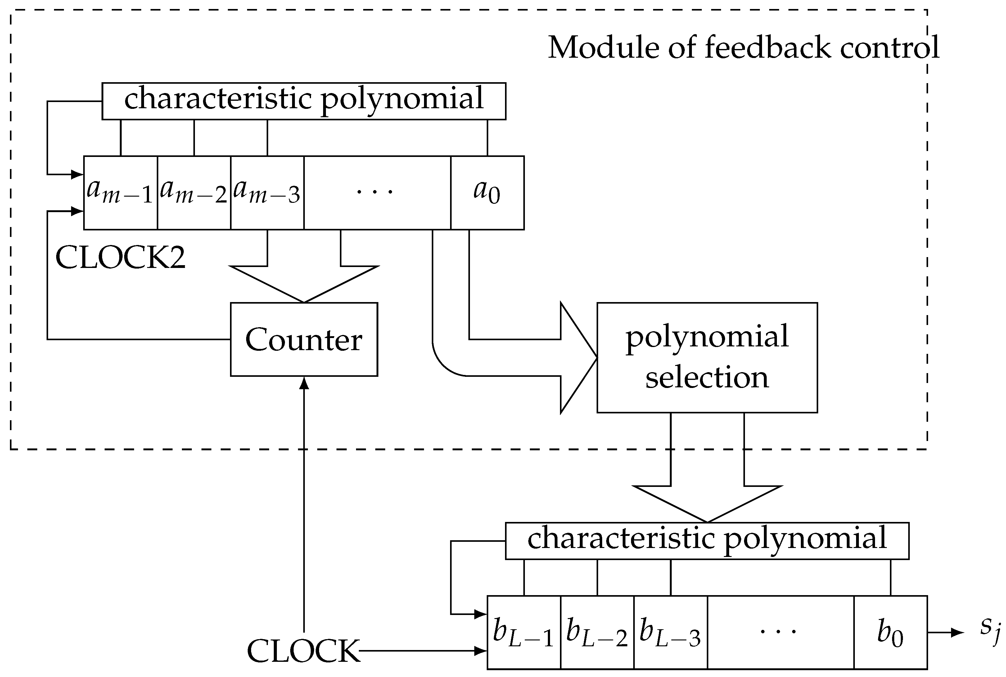
In this work, we consider t-interleaved sequences obtained interleaving PN-sequences from different primitive polynomials with the same degree. Note that these t-interleaved sequences can be seen as the output sequences of a keystream generator where, at each clock pulse, we obtain at the same time the output of t different LFSRs. That is, at each instant $t_i$, the output bits are $\{u_{t_i}^{\left(1\right)},u_{t_i}^{\left(2\right)},\dots ,u_{t_i}^{\left(t\right)}\}$. Therefore, the interleaving method, in this case, could be considered as the concatenation of the output of t LFSRs at each instant of time. On the other hand, this interleaving method is very similar to the generation method of a DLFSR. A DLFSR (Dynamic Linear Feedback Shift Register) is a type of LFSR in which the characteristic polynomial changes at certain clock pulse [17,18]. In Figure 2, we represent a DLFSR that consists of a main LFSR and an additional control module. This module manages the characteristic polynomial used at each instant of time. The sequences generated by a DLFSR can be considered as the concatenation of segments of different PN-sequences. The purpose of a DLFSR is to generate sequences with larger periods and higher linear complexity than the ones produced by a single LFSR [19,20]. To carry out this task, the control module modifies different feedback parameters to generate a different sequence. Our interleaving method can be seen as a DLFSR where the characteristic polynomial changes depending on the counter module, i.e., at each clock pulse, we consider a different primitive polynomial. In Figure 3, we can check the generation of a four-interleaved sequence. At each clock pulse, one bit is generated from the corresponding LFSR in that instant, and then, we jump from the actual polynomial to the next one. Thus, we obtain our interleaved sequence concatenating the individual outputs of each one of the LFSRs at each instant of time.

3. Interleaving PN-Sequences with Different Characteristic Polynomials

In this section, we analyze the interleaving of PN-sequences obtained from different polynomials with the same degree.

Consider t maximal-length LFSRs, notated $R_1$, $R_2$,…, $R_t$, with primitive characteristic polynomials $p_1\left(x\right),$$p_2\left(x\right),\dots ,p_t\left(x\right)$, respectively, and all of them with degree L. Given the PN-sequence $\left\{a_i^{\left(k\right)}\right\}$, generated by $R_k$, for $k=1,2,\dots ,t$, the corresponding t-interleaved sequence $\left\{s_j\right\}$ is obtained as follows

$$\left\{s_j\right\}=\{a_0^{\left(1\right)},a_0^{\left(2\right)},\dots ,a_0^{\left(t\right)},a_1^{\left(1\right)},a_1^{\left(2\right)},\dots ,a_1^{\left(t\right)},\dots ,a_{L-1}^{\left(1\right)},a_{L-1}^{\left(2\right)},\dots ,a_{L-1}^{\left(t\right)},\dots \}.$$

From now on, we only consider t-interleaved sequences obtained with different polynomials of the same degree.

The following result provides the value of the $LC$ for the t-interleaved sequences. Moreover, it allows us to obtain their characteristic polynomials.

Theorem 3

([21], Theorem 1). The linear complexity of the sequence generated interleaving t PN-sequences produced by different primitive polynomials $p_1\left(x\right),\dots ,p_t\left(x\right)$ of degree L is $LC=t^{2}L$. Furthermore, the characteristic polynomial is

$$p\left(x\right)=\prod _{i=1}^t{p}_i\left(x^t\right).$$

It is worth noticing that the $LC$ and period are not affected by the initial states.

Example 3.

Consider 3 registers with primitive polynomials $p_1\left(x\right)=1+x^2+x^5$, $p_2\left(x\right)=1+x+x^2+x^4+x^5$ and $p_3\left(x\right)=1+x+x^2+x^3+x^5$. We take the initial states $\left\{11101\right\}$, $\left\{10001\right\}$ and $\left\{10101\right\}$, respectively. The corresponding PN-sequences are

$$\begin{array}{c}\left\{a_i^{\left(1\right)}\right\}:\left\{1110101000010010110011111000110\right\}\\ \left\{a_i^{\left(2\right)}\right\}:\left\{1000100101011000011100110111110\right\}\\ \left\{a_i^{\left(3\right)}\right\}:\left\{1010100011101111100100110000101\right\}.\end{array}$$

If we interleave these three PN-sequences, we obtain a sequence with period $T=93$ and $LC=45$:

$$\begin{array}{c}\{111100101000111000100010001011001110011001101\\ 001101110010011100100111111100010010010111110001\}\end{array}$$

Using the Berlekamp–Massey algorithm [22], it is possible to check that the characteristic polynomial of this sequence is

$$\begin{array}{cc}\hfill p\left(x\right)& =1+x^9+x^{24}+x^{27}+x^{39}+x^{42}+x^{45}\hfill \\ \hfill & =p_1\left(x^3\right)·p_2\left(x^3\right)·p_3\left(x^3\right)\hfill \end{array}$$

with

$$\begin{array}{cc}\hfill p_1\left(x^3\right)& =1+x^6+x^{15}=(x^5+x^4+x^3+x+1)(x^{10}+x^9+x^7+x^5+x^2+x+1)\hfill \\ \hfill p_2\left(x^3\right)& =1+x^3+x^6+x^{12}+x^{15}=(x^5+x^4+x^3+x^2+1)(x^{10}+x^9+x^7+x^2+1)\hfill \\ \hfill p_3\left(x^3\right)& =1+x^3+x^6+x^9+x^{15}=(x^5+x^3+1)(x^{10}+x^8+x^6+x^5+1)\hfill \end{array}$$

where all three polynomials of degree 5 are primitive and those of degree 10 are irreducible.

The next result is a particular case of Theorem 3 for the case in which t is a power of 2.

Corollary 2.

Let t be a power of two. Then, the characteristic polynomial of a t-interleaved sequence produced by t different primitive polynomials $p_1\left(x\right),\dots ,p_t\left(x\right)$ of degree L is

$$p\left(x\right)={[p_1\left(x\right)·p_2\left(x\right)\cdots p_{t-1}\left(x\right)·p_t\left(x\right)]}^t.$$

Proof. 

Let $t=2^r$ for r be a positive integer. The result is an immediate consequence of the fact that $p_i\left(x^{2^r}\right)=p_i{\left(x\right)}^{2^r}$ in ${\mathbb{F}}_2$. □

Next, we show different examples of the generation of t-interleaved sequences. We analyze their $LC$ and their characteristic polynomials depending on the choice of the initial primitive polynomials.

In the following example, we obtain a $four$-interleaved sequence corresponding to two primitive polynomials and their corresponding reciprocal polynomials.

Example 4.

Consider $four$ registers with primitive polynomials $p_1\left(x\right)=1+x^2+x^5$, $p_2\left(x\right)=1+x^3+x^5$, $p_3\left(x\right)=1+x^2+x^3+x^4+x^5$ and $p_4\left(x\right)=1+x+x^2+x^3+x^5$. We observe that $p_2\left(x\right)$ and $p_4\left(x\right)$ are the reciprocal polynomials of $p_1\left(x\right)$ and $p_3\left(x\right)$, respectively. We take the initial states $\left\{01101\right\}$, $\left\{10001\right\}$, $\left\{10001\right\}$, and $\left\{00110\right\}$, respectively. The corresponding PN-sequences are

$$\begin{array}{c}\left\{a_i^{\left(1\right)}\right\}:\left\{0110111010100001001011001111100\right\}\\ \left\{a_i^{\left(2\right)}\right\}:\left\{1000111110011010010000101011101\right\}\\ \left\{a_i^{\left(3\right)}\right\}:\left\{1000101011010000110010011111011\right\}\\ \left\{a_i^{\left(4\right)}\right\}:\left\{0011000010110101000111011111001\right\}.\end{array}$$

If we interleave these four PN-sequences, we obtain a sequence with period $T=124$ and $LC=80$:

$$\begin{array}{c}\{01101000100100011110110011100100111100101001011101000001010010\\ 01001001101000000110111001010000111111101111111111110000100111\}\end{array}$$

Using the Berlekamp–Massey algorithm [22], it is easy to check that the characteristic polynomial of this sequence is

$$\begin{array}{cc}\hfill p\left(x\right)& ={\left[p_1\left(x\right)·p_2\left(x\right)·p_3\left(x\right)·p_4\left(x\right)\right]}^4\hfill \\ \hfill & ={(1+x^2+x^5)}^4{(1+x^3+x^5)}^4{(1+x^2+x^3+x^4+x^5)}^4{(1+x+x^2+x^3+x^5)}^4\hfill \\ & =1+x^4+x^8+x^{12}+x^{20}+x^{32}+x^{36}+x^{40}+x^{44}+x^{48}+x^{60}+x^{68}+x^{72}+x^{76}+x^{80}.\hfill \end{array}$$

In this example, the $LC$ does not depend on the initial states; its value is always 80. Moreover, if we consider different primitive polynomials of degree 5, the value of $LC$ remains the same.

The next example shows a case where there are no reciprocal polynomials.

Example 5.

Consider now four registers with primitive polynomials $p_1\left(x\right)=1+x+x^7$, $p_2\left(x\right)=1+x^3+x^7$, $p_3\left(x\right)=1+x+x^2+x^3+x^7$ and $p_4\left(x\right)=1+x^2+x^3+x^4+x^7$, with initial states $\left\{1010001\right\},\left\{0111011\right\},\left\{1101001\right\},and\left\{1100101\right\},$ respectively. If we interleave the four PN-sequences generated by the previous polynomials, we obtain a sequence with period 508 (the same as that of the SG with polynomials of degree 3 and 7) and $LC=112$, which is four times higher than that of the SG:

$$\begin{array}{c}\{10110111110001100001010011111110110010100001010010000110010100111010011010\hfill \\ 101000011100111001101110100011100101111011001100101111101010111101110000011\hfill \\ 000001101000010010111111110100101010000011011010001011111100011001110001001\hfill \\ 001111011110000110000110110110000110100111101011100101101100111000010011010\hfill \\ 111001100010110000110011010000101101010011001000111001010111000100100101111\hfill \\ 010110011111100100100001101010001011011000110010111011100111110111000101010\hfill \\ 11001100000100100000101010001010110110111010101001100100010\}.\hfill \end{array}$$

The characteristic polynomial of the sequence is given by

$$\begin{array}{cc}\hfill p\left(x\right)& ={[p_1\left(x\right)·p_2\left(x\right)·p_3\left(x\right)·p_4\left(x\right)]}^4\hfill \\ \hfill & ={\left[(1+x+x^7)(1+x^3+x^7)(1+x+x^2+x^3+x^7)(1+x^2+x^3+x^4+x^7)\right]}^4\hfill \\ \hfill & ={(1+x^2+x^5+x^7+x^8+x^9+x^{11}+x^{12}+x^{15}+x^{16}+x^{17}+x^{18}+x^{24}+x^{25}+x^{28})}^4.\hfill \end{array}$$

The next example shows that the polynomials must be all different to achieve the maximal complexity.

Example 6.

Consider the primitive polynomials $p_1\left(x\right)=p_2\left(x\right)=1+x^2+x^5$, $p_3\left(x\right)=1+x+x^2+x^3+x^5$ and $p_4\left(x\right)=1+x^2+x^3+x^4+x^5$ and consider the initial states $\left\{10111\right\}$, $\left\{11010\right\}$, $\left\{00011\right\}$, and $\left\{10110\right\}$, respectively. The corresponding $four$-interleaved sequence has the following form:

$$\begin{array}{c}\{11010100100111111010011110000010101000100111001100001100001101\hfill \\ 00110000111011110101010101110011111001101110100100011000011110\}\hfill \end{array}$$

This sequence has period $T=124$ and $LC=60$, which is not the maximal vale (80) for this parameter. The characteristic polynomial is given by:

$$p\left(x\right)={\left[p_1\left(x\right)p_3\left(x\right)p_4\left(x\right)\right]}^4=1+x^4+x^8+x^{16}+x^{20}+x^{24}+x^{36}+x^{56}+x^{60}$$

Notice that in this case, the primitive polynomial is not the product of all four polynomials; this is due to the fact that $p_1\left(x\right)=p_2\left(x\right)$.

In

Table 1. $LC$ of the interleaving sequences of t primitive polynomials of degree L.

	L	5	6	7	8	9
t
4		80	96	112	128	144
5		125	150	175	200	225
6		180	216	252	288	324
7		245	294	343	392	441
8		320	384	448	512	576

, we can check the values of the $LC$ of t-interleaved sequences using PN-sequences from different polynomials of degree L. It is worth recalling that there are only six primitive polynomials of degree 5 and six of degree 6. It means that when we construct seven-interleaved sequences or eight-interleaved sequences, we have to consider at least one repeated polynomial. Therefore, the values in red in Table 1 are just upper bounds, since, as we saw in Example 6, when the polynomials are not different, we risk having a sequence without maximal $LC$.

4. Comparison with Other Sequence Generators

In this section, we analyze briefly the advantages of our t-interleaved sequences compared with the sequences obtained from generators with similar parameters.

1

Shrinking generator

Given two primitive polynomials of degree $L_1$ and $L_2$, the linear complexity of the shrunken sequence satisfies: $2^{L_1-2}<LC\le L_2·2^{L_1-1}$ and $T=(2^{L_2}-1)2^{L_1-1}$. In this case, the sequence is obtained interleaving $2^{L_1-1}$ shifted versions of the same PN-sequence.

If we interleave $2^{L_1-1}$ PN-sequences generated by different primitive polynomials of degree $L_2$, the linear complexity of the resultant sequence is $LC=L_2·2^{2(L_1-1)}$, which is much higher than that of the SG. Notice that the period and the number of ones remain the same.

In the following example, we compare the shrunken sequence and the corresponding t-interleaved with similar parameters. We see that the $LC$ of the t-interleaved sequence is greater.

Example 7.

Consider the SG composed of two registers of length $L_1=3$ and $L_2=5$. In this case, the shrunken sequence is made up by interleaving four shifted versions of the same PN-sequence generated by a primitive polynomial of degree 5. The period of the shrunken sequences in this case is $T=124$ and $LC\le 20$.

If we consider again Example 4, we interleave four PN-sequences produced by primitive polynomials of degree 5. The resultant sequence has period 124 (the same as that of the SG with polynomials of degree 3 and 5) and $LC=80$, which is four times higher than that of the SG.

2

t-interleaved sequences with the same polynomial

In [12], the authors analyze the t-interleaved sequences obtained interleaving shifted versions of the same PN-sequence produced by a primitive polynomial $p\left(x\right)$ of degree L. They determine the period and the linear complexity of the t-interleaved sequences for some particular cases of t. They also study an upper bound for the $LC$ and the period of t-interleaved PN-sequences. In [21], the authors study different cases of interleaving sequences, analyzing the $LC$ and the characteristic polynomials of the resultant sequences. The next theorem is a consequence of Theorem 2 in [21] and the results obtained in [12].

Theorem 4.

[12,21] Consider a primitive polynomial $p\left(x\right)$ of degree L. If we interleave t-shifted versions of the same PN-sequence of period $T=2^L-1$, then the resultant t-interleaved sequence has an $LC\le t·L$ and period $T\le t·\left(2^L-1\right)$.

In the following example, we compare a t-interleaved sequence obtained using one primitive polynomial $p\left(x\right)$ of degree L with a corresponding t-interleaved sequence, with similar parameters, obtained using t different primitive polynomials $p_i\left(x\right)$ of degree L, $i=1,\dots ,t$. We see that the $LC$ of the t-interleaved sequence with different polynomials is greater.

Example 8.

Consider any $four$-interleaved sequence obtained with a primitive polynomial of degree 5 and $four$ shifted versions of the corresponding PN-sequence. In this case, the period of the sequences is $T\le 124$ and $LC\le 20$.

Consider the primitive polynomials of degree 5 given in Example 4 and interleave $four$ different PN-sequences produced by these polynomials. The resultant sequences have period 124 and $LC=80$. If we compare both types of $four$-interleaved sequence, we have that using different polynomials for the construction provides higher values for the $LC$, in this case, four times larger.

In

Table 2. Values for the $LC$ and the period T of t-interleaved sequences obtained from one single primitive polynomial of degree L compared with the values taking different polynomials.

	t Different Polynomials		1 Polynomial
$(\mathit{t},\mathit{L})$	$\mathit{LC}$	$\mathit{T}$	$\mathit{LC}$	$\mathit{T}$
(8,16)	1024	524,280	128	524,280
(8,17)	1088	1,048,568	136	1,048,568
(8,18)	1152	2,097,144	144	2,097,144
(8,19)	1216	4,194,296	152	4,194,296
(8,20)	1280	8,388,600	160	8,388,600

, we have a comparison between the values of $LC$ and T for our t-interleaved sequences and the values for the sequences obtained in [12] (using shifted versions of the same PN-sequence, that is, with the same characteristic polynomial). First of all, notice that the values for the same polynomial are upper bounds (it depends on the initial state), while the values for our sequences are exact (regardless the initial state). Note that values of $LC$ are higher in our sequences.

In order to complete this comparison, in the next section, we perform a statistical study on the randomness of our t-interleaved sequences, and we compare these results with the ones obtained for t-interleaved sequences obtained with shifted versions of the same PN-sequence (which includes the shrunken sequence), that is, using always the same characteristic polynomial.

5. Statistical Analysis of T-Interleaved Sequences

RNGs should be designed and selected based on a solid theoretical analysis of their mathematical structure. In our algorithm, we interleave PN-sequences to hide and delete their linearity. Once our generator is designed and implemented, the next step is to submit it to empirical statistical tests in order to detect statistical deficiencies. In the study of RNGs, different quality criteria can be used. However, three basic properties of a random bit sequence $\left\{s_i\right\}$ should be achieved:

• Unpredictability: Having k consecutive elements of $\left\{s_i\right\}$ should not give any information about the next element $k+1$ of the sequence.
• Uniformity: Given any subsequence of $\left\{s_i\right\}$, there should be nearly equal number of 1’s and 0’s.
• Independence: Each element of $\left\{s_i\right\}$ is independent from other elements.

There is no mathematical proof that ensures the randomness of a bit sequence; however, there exists a huge number of empirical tests to determine if a sequence is random enough and secure to be used in cryptography [23]. If the sequences produced by a particular generator pass the statistical tests, then this could be accepted as a generator of random sequences. Otherwise, if any of the tests fail, then it means the generator is not good and must be rejected.

• Golomb’s Randomness Postulates

Golomb’s postulates constitute a base for randomness tests, since they were one of the first attempts to establish some necessary conditions for a periodic pseudo-random sequence to look random. Sequences satisfying the three properties are called PN-sequences. The sequences produced by LFSRs are PN-sequences in these terms. At present, these conditions are far from being sufficient for such sequences to be considered random. However, there are diverse ways and tools that allow us to analyze the randomness of the sequences.

>From now on, we consider $\left\{s_i\right\}$ a binary sequence of period T. A run of $\left\{s_i\right\}$ is defined as a maximal subsequence of consecutive bits of either all ones or all zeros. A run of zeroes is called a gap, and a run of ones is called a block. Golomb’s postulates are defined as follows:

(R1)

In a period of $\left\{s_i\right\}$, the number of ones should differ from the number of zeros by at most 1. In other words, the sequence should be balanced.

(R2)

In a period of $\left\{s_i\right\}$, at least $\frac{1}{2}$ of the all runs of zeroes or ones should have length one, at least $\frac{1}{4}$ should have length 2, at least $\frac{1}{8}$ should have length 3, and so on. Moreover, for each one of these lengths, there should be (almost) equally many gaps and blocks.

(R3)

The autocorrelation function $C\left(\tau \right)$ should be two valued. That is, for some integer k and for all $\tau =0,1,2,\dots ,T-1$

$$\begin{array}{c}\hfill C\left(\tau \right)=\frac{1}{T}\sum _{i=0}^{T-1}{(-1)}^{(s_i+s_{i+\tau })}=\left\{\begin{array}{cc}1& \mathrm{if}\tau =0,\hfill \\ \frac{k}{T}& \mathrm{if}1\le \tau \le T-1.\hfill \end{array}\right.\end{array}$$

(2)

Any of Golomb’s randomness postulates are analyzed through the statistical tests package FIPS 140-2 [24], as we study in Section 5.2.

In this section, we include diverse ways to analyze the randomness of our sequences. On the one hand, in Section 5.1, we present some visual results where, through different graphs, we could understand the behavior of the generated sequences. On the other hand, in Section 5.2, we evaluate various batteries of statistical tests, which help us to determine if our generator could be considered random. The generator and the battery of tests were implemented with Matlab R2020b in a Windows 10 environment in a 64 bits PC with CPU Intel Core i7, at 3 GHz. We check a great quantity of t-interleaved sequences, with $3\le t\le 8$ and with polynomials of degree up to 27.

5.1. Simple Visual Analysis

In this subsection, we examine our random number generator creating a visualization of the sequences it produces. We study the autocorrelation, the return map, the chaos game, and the Lyapunov exponent. This type of approach should not be considered as an exhaustive or formal analysis. However, it is an interesting and easy way to get a rough impression of the performance of the generator.

• Autocorrelation

The autocorrelation function, defined in expression (2), measures the amount of similarity between the sequence $\left\{s_i\right\}$ and its shifted version by $\tau$ positions. If $\left\{s_i\right\}$ is a random periodic sequence of period T, then $|T·C(\tau \left)\right|$ can be expected to be quite small for all values of $\tau$ with $0<\tau <T$.

This function is a mathematical tool very useful for finding repeated patterns. It analyzes different sections of a message and compares them to find similarities. Moreover, it allows measuring the linear relationship between random variables of processes separated a certain distance. The first autocorrelation coefficient is always equal to 1, and the other coefficients must have the smallest amplitude possible, so that the sequence can be considered random.

In Figure 4, we compare the autocorrelation values for two 8-interleaved sequences. In Figure 4a, we show the results for an eight-interleaved sequence with eight different primitive polynomials of degree $L=16$. We observe that the values are almost zero except for the first value which is 1, as would be expected for a random sequence. Obtaining these results provides an indication about the randomness of the sequence but not the certainty. That is, this does not guarantee that it was indeed produced by a random bit generator, but it means that we can continue checking it. However, in Figure 4b, we represent the results for a eight-interleaved sequence with the same polynomial of degree $L=16$. We can observe in the graph how the values increase for some shifts of the sequence with itself. This allows us to deduce the existence of certain autocorrelation in this sequence.

• Chaos Game

Chaos game [25,26,27] is a method that converts a one-dimensional sequence into a sequence in two dimensions providing a very provocative visual representation, which reveals some of the statistical properties of the sequence under study. >From this graphical tool, we can visually look for patterns in the sequences generated by a random number generator.

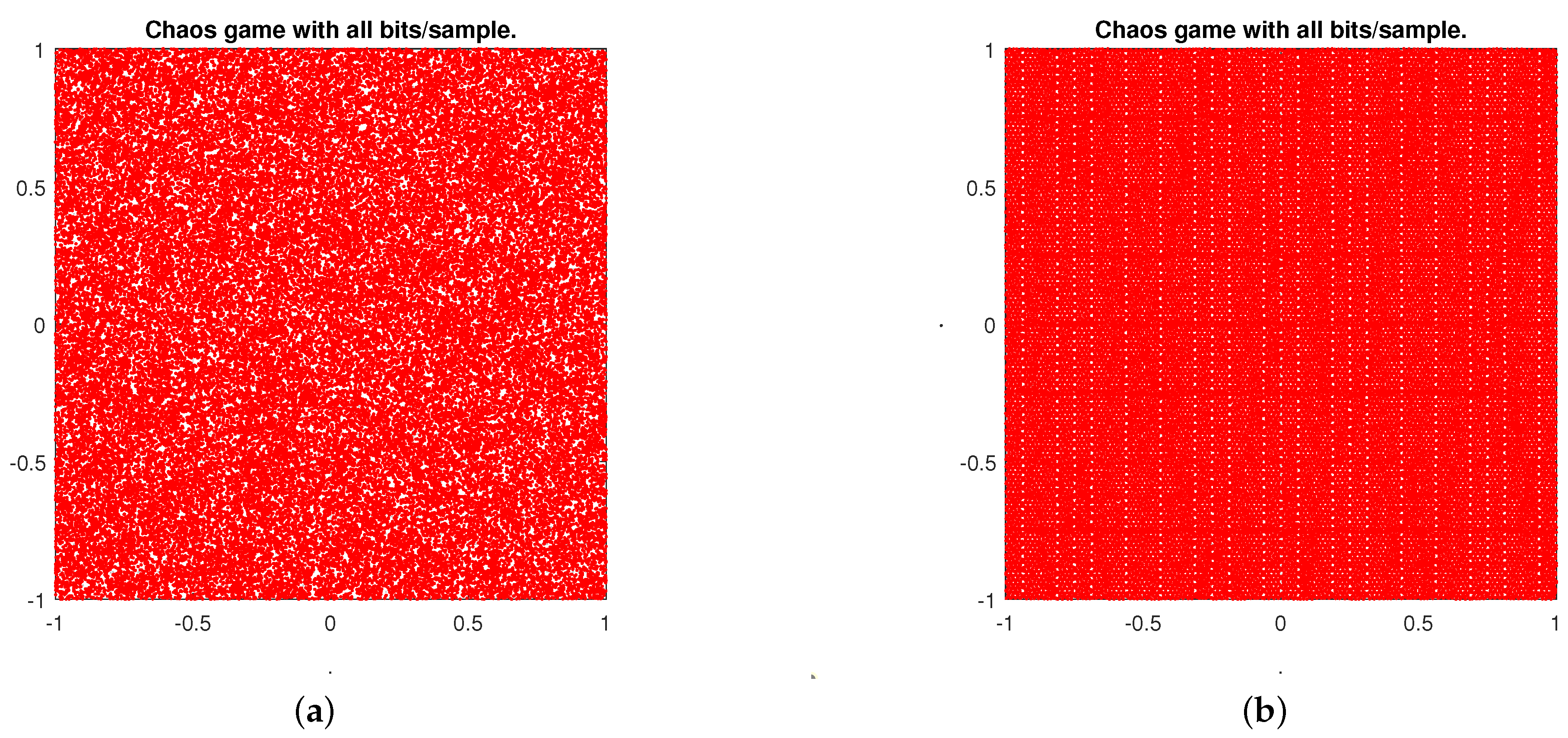
Figure 5 shows the Chaos maps of two eight-interleaved sequences with polynomials of degree 16. In Figure 5b, we have the Chaos map of an eight-interleaved sequence generated with one single polynomial. We can observe the lack of randomness in this sequence, since it presents a clear pattern. However, in Figure 5a, we have the Chaos map of an eight-interleaved sequence using different polynomials where we observe a disordered cloud, without patterns. It means that there is an indication of a Chaos map but not certainty. That is, it does not assure the randomness of our sequence, but we can continue with the analysis of this generator.

A practical method of determining whether a system is chaotic or not is the calculation of the Lyapunov exponent, which we study in the next section.

• Lyapunov exponent

Lyapunov exponent is an essential tool and a useful analytical metric to characterize the chaos. An important property of chaos is its very sensitive dependence on initial condition. Lyapunov exponent is used as a quantitative measure for this dependence.

Lyapunov exponent of a dynamical system is a quantity that characterizes the rate of separation of infinitesimally close trajectories $Z\left(t\right)$ and $Z_0\left(t\right)$ in phase space

$$|Z\left(t\right)-Z_0\left(t\right)|\approx |Z\left(0\right)-Z_0\left(0\right)|e^{\lambda t}.$$

The exponent $\lambda$ measured for a long period of time (ideally $t\to \infty$) is the Lyapunov exponent.

Next, we consider the definition of Lyapunov exponent given for sequences in [28]. Let $d_0$ be the measure of the initial distance between two sequences and $d_t$ be the distance between the same sequences but after t iterations. We define Lyapunov exponent (LE) as:

$$LE=\frac{1}{t}ln\left(\left|\frac{d_t}{d_0}\right|\right).$$

It is desirable that two very close initial conditions provide very different trajectories (sequences). If $LE$ is greater than zero, the distance between two close initial conditions rapidly increases in the time, which means there exists an exponential divergence of the trajectories of a chaotic system. This value gives an idea of how different the sequences are generated by similar seeds, which is a very important feature to avoid attacks on the key of the generator. However, if $LE=0$, the sequences decrease their distance, and they tend to join and be confused in one. The system converges, and it is not at all random.

We can use the Hamming distance (which indicates the number of bit positions in which both sequences differ) instead of the logarithm of the Euclidean distance in the Lyapunov exponent, and it is called the Lyapunov Hamming Exponent (LHE). If two numbers are identical, then its LHE value will be 0. Nevertheless, if all the bits of both numbers are different, then its LHE will be $LHE={log}_{2}m={log}_2{2}^n=n$, where n is the number of bits with which the numbers are encoded.

Obtaining the Lyapunov Hamming exponent for the chosen sequence is done by calculating the average of the LHE between every two consecutive numbers of the sequence. The best value will be $n/2$.

For this case, we take $n=8$, so the best value is 4. Next, we show the value obtained for a eight-interleaved sequence with polynomials of degree $L=20$

Lyapunov Hamming exponent, ideal	=	4
Lyapunov Hamming exponent, real	=	$4.0001$
Absolute desviation from ideal	=	2.2889 × 10${}^{-5}$

Hence, the proposed generator passes this test.

All the t-interleaved sequences with different polynomials analyzed have passed this test.

• Return map

In Information Theory, the entropy of a sequence is a measure of the amount of information of a process in bits; or it is a measure of the diversity of the elements in the sequence. It is computed from the frequencies of each element of the alphabet in the sequence.

The return map is useful to visually measure the entropy of the sequence above defined; that is, it allows us to detect the existence of some useful information about the parameters used in the design of pseudo-random generators [29].

The return application consists of drawing a two-dimensional graph of the points of the sequence $\left\{s_i\right\}$ as a function of $\left\{s_{i-1}\right\}$. The result should be a distribution of points where you can guess no trend, no shape, no line, no symmetry, and no pattern, as happens in the Chaos map.

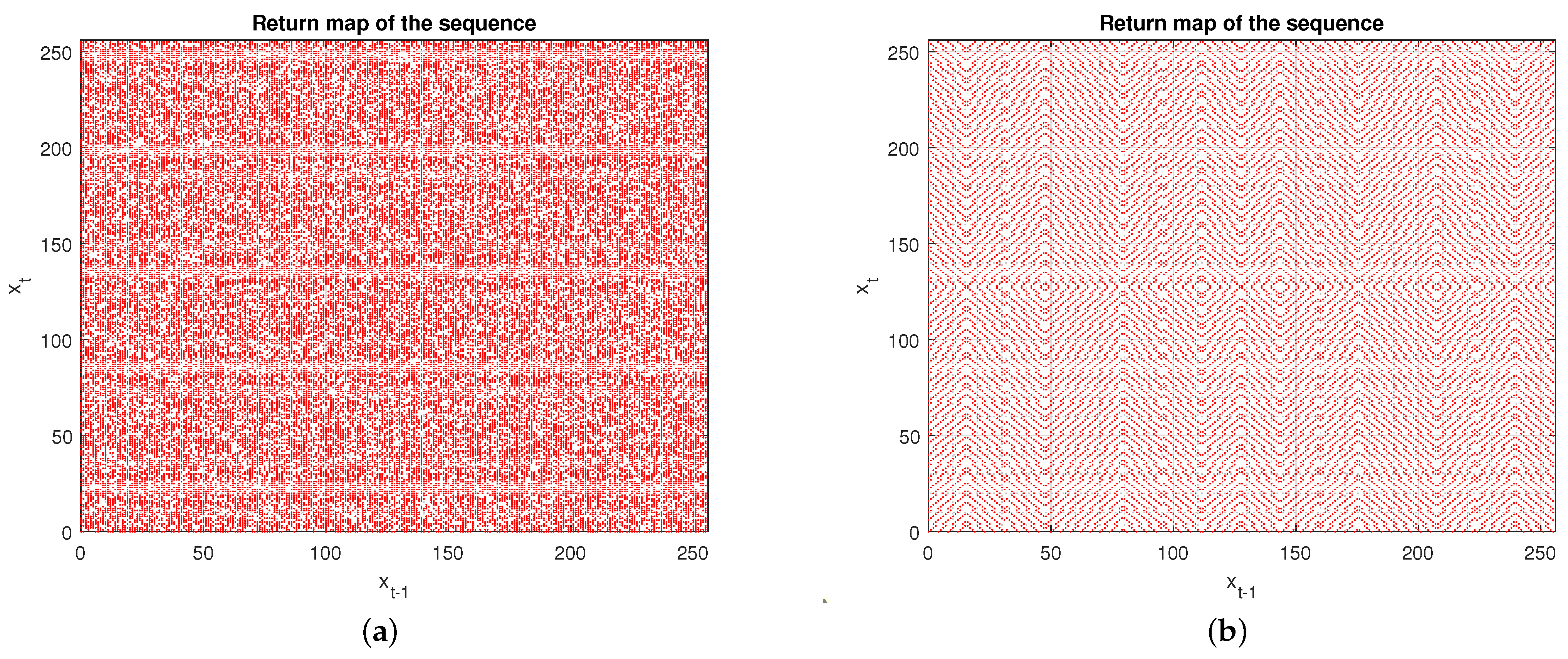
In Figure 6, we represent the return maps of two eight-interleaved sequences with polynomials of degree 16. In Figure 6a, we have the return map of an eight-interleaved sequence using different polynomials. We observe a disordered cloud, without patterns, which, in principle, does not provide any useful information for the cryptanalysis of the sequence. It does not mean that our sequence is random, simply that it is not rejected in the randomness analysis. However, in Figure 6b, we represent the return application of an eight-interleaved sequence generated with one single polynomial. We can check that this graph presents a pattern of defined curves, which are repeated. It indicates non-randomness in the sequence.

5.2. Battery of Statistical Tests

Next, we present two of the most important batteries of statistical tests used to evaluate the randomness of the sequences generated by pseudo-random number generators, Diehard and NIST.

• NIST
  The Statistical Test Suite developed by NIST [30] is an excellent and exhaustive document looking at various aspects of randomness in a long sequence of bits. The NIST has documented 15 statistical tests, where FIPS 140-2 package, Maurer’s Universal Test [31] and Lempel–Ziv Compression Test are among them.
  The Frequency Test, Maurer’s Universal Test and Lempel-Ziv Compression have the standard normal as reference distribution. The rest of the tests have the chi-square ${\chi }^2$ as reference distribution. The chi-square and the normal variation is converted into a p-value. If the computed p-value is <0.01, then we conclude that the sequence is non-random. Otherwise, we conclude that the sequence is random.
• FIPS 140-2
  FIPS 140-2 is an U.S. government computer security standard used to approve cryptographic modules issued by the National Institute of Standards and Technology (NIST). It consists of four statistical random number generator tests: the Monobit Test, The Poker Test, The Runs Test and The Long Runs Test. Moreover, we add the Frequency Test within a block, which can be categorized as a frequency test. If a sequence passes all five tests, there is no guarantee that it was indeed produced by a random bit generator. However, if one of the algorithms fails any of these tests, then the other tests are not even applied, and we can not consider our sequence sufficiently random; and, therefore, our generator is not secure in cryptographic terms.
  Each test needs a binary sequence of ${10}^6$ bits. All our sequences have the required length for this analysis.
  • FREQUENCY (MONOBIT) TEST: The focus of the test is the proportion of zeros and ones along the whole sequence. The purpose of this test is to determine whether the number of ones and zeros in a sequence are approximately the same as would be expected for a truly random sequence. The test assesses the closeness of the fraction of ones to $\frac{1}{2}$; that is, the number of ones and zeros in a sequence should be about the same. All subsequent tests depend on the approval of this test.
  • POKER (SERIAL) TEST: Let m be an integer number such that $\lfloor \frac{T}{m}\rfloor \ge 5·2^m$ and let $k=\lfloor \frac{T}{m}\rfloor$. The sequence $\left\{s_i\right\}$ is divided into k non-overlapping parts each one of length m, and let $m_i$ be the number of occurrences of the i-th type of sequence of length m, for $1\le i\le 2^m$. The Poker Test determines if each stream of length m appears approximately the same number of times in $\left\{s_i\right\}$, as would be expected for a random sequence. Note that for $m=1$, the Poker Test is equivalent to the Frequency Test.
  • RUNS TEST: The incidences of runs (for both consecutive zeros and consecutive ones) of all lengths (≥1) in the sample stream should be counted and stored. The purpose of the Runs Test is to determine if the number of runs of different lengths in the sequence $\left\{s_i\right\}$ is as expected for a random sequence. In particular, this test determines whether the oscillation between zeros and ones is too fast or too slow.
  • LONG RUNS TEST: A long run is defined to be a run of length 26 or more (of either zeros or ones). The focus of this test is the longest run of ones within M-bit blocks. Its purpose is to determine whether the length of the longest run of ones within the sequence is consistent with the length of the longest run of ones that would be expected in a random sequence. Note that one irregularity in the expected length of the longest run of ones implies that there is also an irregularity in the expected length of the longest run of zeros. Therefore, only a test for ones is necessary.
  • FREQUENCY TEST WITHIN A BLOCK: The focus of this test is the proportion of ones within M-bit blocks. The purpose is to determine whether the frequency of ones in an M-bit block is approximately $\frac{M}{2}$, as would be expected under an assumption of randomness. For the block size $M=1$, this test degenerates to the Frequency (Monobit) test.
  Frequency Test is defined to check the first postulate of Golomb. The second postulate of Golomb, about the number of runs in sequences, is analyzed in the Runs Tests. Finally, the third postulate gives information about similarities between the sequence and shifted versions of it. If $\left\{s_i\right\}$ is a random sequence, the autocorrelation should be constant.
• Maurer’s Universal Test
  The focus of this test is the number of bits between matching patterns (a measure that is related to the length of a compressed sequence). The purpose of the test is to detect whether or not the sequence can be significantly compressed without loss of information. A significantly compressible sequence is considered to be non-random.
• Lempel–Ziv Compression Test
  The focus of this test is the number of cumulatively distinct patterns (words) in the sequence. The purpose is to determine how far the tested sequence can be compressed; it is considered to be non-random if it can be significantly compressed. A random sequence will have a characteristic number of distinct patterns.
  This test works by reading a sequence of symbols, grouping the symbols into strings, and converting the strings into codes. We get compression because the codes take up less space than the strings they replace. No data are lost when compressing.
  In

  Table 3. p-values of some statistical tests of NIST for t-interleaved sequences with different characteristic polynomials of degree 20.

  	t-Interleaved	3	4	5	6	7	8
  Tests
  Monobit		0.4952	0.4740	0.0493	0.6213	0.5592	0.9745
  Poker		0.9083	0.2742	0.5086	0.0488	0.9960	0.4902
  Runs		0.5402	0.5160	0.4629	0.5946	0.6000	0.9840
  Long Runs		0.5715	0.5823	0.6785	0.8791	0.1204	0.9719
  Frequency block		0.4068	0.2167	0.3672	0.7633	0.3473	0.5089
  Maurer’s		0.6623	0.4129	0.2069	0.8374	0.5539	0.4262
  Lempel-Ziv		0.0931	0.9159	0.0531	0.2314	0.9069	0.9719

  , we present a small sample of the results obtained in the NIST tests here presented. All these values are the average of the results obtained for any sample of t-interleaved sequences studied.
• Diehard
  Diehard battery of tests [32] is a reliable standard for evaluating the randomness of sequences of pseudo-random number generators. This tool is a powerful instrument for the practical evaluation process of cryptographic primitives. It cannot guarantee if your generator can be considered perfectly random, but if it does not pass the test suite, then it is not suitable for cryptographic applications.
  Diehard battery [32] consists of 15 different independent statistical tests, some of them repeated but with different parameters:
  • BIRTHDAY SPACINGS TEST: Choose random points on a large interval. The spacings between the points should be asymptotically exponentially distributed.
  • OPERM5 TEST: Analyze sequences of five consecutive random numbers. The 120 possible orderings should occur with statistically equal probability.
  • BINARY RANK TEST FOR $31\times 31$ MATRICES: The leftmost 31 bits of 31 random integers from the test sequence are used to form a $31\times 31$ binary matrix over the field $\{0,1\}$. The rank is determined. That rank can be from 0 to 31, but ranks less than 28 are rare, and their counts are pooled with those for rank 28. Ranks are found for 40,000 of such random matrices, and a chi-square test is performed on counts for ranks $31,30,29$ and ≤28.
  • BINARY RANK TEST FOR $32\times 32$ MATRICES: The rank of a random $32\times 32$ matrix is identified. Ranks less than 29 are rare. Chi-square tests are performed on the ranks $32,31,30$ and less than or equal to 29. This is repeated 40,000 times.
  • BINARY RANK TEST FOR $6\times 8$ MATRICES: The rank of a random $6\times 8$ matrix is identified. Ranks less than 4 are rare. Chi-square tests are performed on the ranks $6,5$ and less than or equal to 4. This is repeated 100,000 times.
  • BITSTREAM TEST: Consider each bit as a single letter $\left(0\mathrm{or}1\right)$. In a rolling group of 20 bits, count the number of 20-bit permutations out of $2^{21}$ 20-bit groups. As there are $2^{20}$ possible 20-bit permutations, count how many are missing, which should be normally distributed. This test is repeated 20 times.
  • OPSO, OQSO and DNA TESTS:

    (a)

    OPSO TEST: This is the overlapping-pairs-sparse-occupancy test. Each set of 5 bits is considered a ’letter’; thus, there are 1024 letters in the ’alphabet’. Two-letter words are taken from each 32-bit integer and are counted. As there are $2^{21}$ possible two-letter words, the missing words are identified and should be normally distributed.

    (b)

    OQSO TEST: A variant that uses four-letter words.

    (c)

    DNA TEST: A variant where there are only four letters in the alphabet, and each letter is two bits.

  • COUNT-THE-1s TEST: A specific byte from each integer is chosen to represent a letter. There are five possible letters, each chosen by counting the number of 1’s in the byte: $0,1,2=A;3=B;4=C;5=D;6,7,8=E$. The five probabilities are therefore $37,56,70,56$ and 37 over 256, respectively. Five integer sequences are selected on a rolling basis, and counts are made on word frequencies. A covariance matrix is formed.
  • PARKING LOT TEST: Randomly place unit circles in a $100\times 100$ square. A circle is successfully parked if it does not overlap an existing successfully parked one. After 12,000 tries, the number of successfully parked circles should follow a certain normal distribution.
  • MINIMUM DISTANCE TEST: In a square of size 10,000 × 10,000, randomly select 8000 points. Find the minimum distance between the pairs. The square of this distance should be exponentially distributed with a mean close to $0.995$. This is repeated for 100 random selections of 8000 points.
  • RANDOM SPHERES TEST: Randomly choose 4000 points in a cube of edge 1000. Center a sphere on each point, whose radius is the minimum distance to another point. The smallest sphere’s volume should be exponentially distributed with a certain mean.
  • SQUEEZE TEST: Multiply $2^{31}$ by random floats on $(0,1)$ until you reach 1. Repeat this 100,000 times. The number of floats needed to reach 1 should follow a chi-square distribution.
  • OVERLAPPING SUMS TEST: Generate a long sequence of random floats on $(0,1)$. Add sequences of 100 consecutive floats. The sums should be normally distributed with characteristic mean and variance.
  • RUNS TEST: Generate a long sequence of random floats on a $[0,1)$ distribution. Ascending and descending runs should follow a certain covariance matrix. This is repeated 10 times for sequences of length 10,000.
  • CRAPS TEST: Play 200,000 games of craps, counting the wins and the number of throws per game. Each count should follow a chi-square distribution.
  Note that The Count-The-1s and the OPSO tests are both sometimes known as the Monkey Test. These statistical tests are designed to test the null hypothesis $H_0$, which states that the input sequence is randomly generated. If the hypothesis is not rejected in all the tests, then it is implied that the input sequences are random. Most of the tests in DIEHARD return a p-value or the KS p-value (given by the Kolmogorov–Smirnov test), which should be uniform on $[0,1)$ if the input file contains truly independent random bits. It is considered that a bit stream really fails when it obtains p-values of 0 or 1 to six or more places.
  Testing Diehard battery of tests for a hundred eight-interleaved sequences with different polynomials of degree 24, we say that Diehard does not show any weakness. >From the results of

  Table 4. Diehard battery of tests results for an eight-interleaved sequence with different characteristic polynomials of degree 24.

  Test Name	p-Value	Result	Test Name	p-Value	Result
  Birthday spacing	0.770936	Pass	OQSO	0.8197	Pass
  	0.747460			0.1329
  	0.989202			0.5293
  	0.774785			0.6284
  	0.576802			0.7687
  	0.176450			0.0969
  	0.874796			0.7288
  	0.139735			0.9149
  	0.514557			0.9812
  Overlapping	0.974948	Pass	OQSD	0.7603	Pass
  permutations	0.759794			0.6207
  Binary ranks $31\times 31$	0.752307	Pass		0.8554
  Binary ranks $32\times 32$	0.934338	Pass		0.3293
  Binary ranks $6\times 8$	0.445734	Pass		0.0179
  Bit stream (Monkey tests)	0.76389	Pass		0.7859
  	0.13337			0.4336
  	0.67455			0.1403
  	0.49876			0.7540
  	0.88496			0.3442
  	0.96748			0.1236
  	0.07041			0.1888
  	0.08609			0.8394
  	0.67958			0.6233
  	0.61726			0.1351
  	0.78081			0.4005
  	0.61369			0.4097
  	0.80996			0.4941
  	0.88405			0.8206
  	0.35224		DNA	0.5756	Pass
  	0.62968			0.7611
  	0.53228			0.5149
  	0.17966			0.8418
  	0.02605			0.9799
  	0.16593			0.2000
  OPSO	0.8834	Pass		0.6843
  	0.7423			0.8916
  	0.2625			0.2560
  	0.5394			0.2569
  	0.5394			0.0096
  	0.6175			0.2598
  	0.2614			0.1103
  	0.6739			0.2117
  	0.7986			0.5963
  	0.6588			0.3547
  	0.7102			0.4503
  	0.4069			0.5184
  	0.8906			0.9202
  OPSO	0.4968	Pass	DNA	0.0457	Pass
  	0.1266			0.8440
  	0.1259			0.9479
  	0.8229			0.6468
  	0.4243			0.3536
  	0.3429			0.6446
  	0.6911			0.0831
  	0.1838			0.7538
  	0.2961			0.7575
  	0.2145			0.9951
  Count-the-1’s (stream of bytes)	0.476036	Pass		0.5849
  	0.572657			0.2852
  Count-the-1’s (specific bytes)	0.	Pass	Parking lot	0.407931	Pass
  	0.453489		Minimum distance	0.752286	Pass
  	0.531694		3D Spheres	0.947691	Pass
  	0.476337		Squeeze	0.990622	Pass
  	0.115181		Overlapping sums	0.276467	Pass
  	0.238283		Runs	0.276783	Pass
  	0.248038			0.893007
  	0.170200			0.908305
  	0.595302			0.913183
  	0.167417		Craps	0.995956	Pass
  	0.574701			105,661
  	0.384873
  	0.944743
  	0.955924
  	0.210026
  	0.142320
  	0.717744
  	0.191102
  	0.728247
  	0.297792
  	0.971290
  	0.323464
  	0.408101
  	0.013264
  	0.859849

  of a particular sequence, we can check that all the values are in the appropriate range.

6. Conclusions

Interleaving sequences is a way to increase the linear complexity of such sequences and to break the linearity just in case of working with PN-sequences. In this paper, we analyze the randomness of the sequences obtained by interleaving PN-sequences generated by different characteristic polynomials with the same degree. According to the obtained results, these sequences achieve the maximal possible linear complexity and, in terms of randomness, they are better than the sequences obtained interleaving PN-sequences with the same polynomial. Therefore, they seem to be suitable for applications in cryptography. As future work, we would like to apply more batteries of tests to our sequences and study what happens if we interleave PN-sequences with different periods. In this last case, we are not sure how the different periods can affect the resultant sequence. We need to perform a deep study in order to achieve some conclusions.

References

- Gallegos-Segovia, P.; Bravo-Torres, J.; Argudo-Parra, J. Internet of things as an attack vector to critical infrastructures of cities. In Proceedings of the 2017 International Caribbean Conference on Devices, Circuits and Systems (ICCDCS), Cozumel, Mexico, 5–7 June 2017; pp. 117–120. [Google Scholar]
- Biryukov, A.; Perrin, L. State of the Art in Lightweight Symmetric Cryptography. Cryptology ePrint Archive, Report 2017/511. 2017. Available online: https://ia.cr/2017/511 (accessed on 3 April 2022).
- Chin, W.; Li, W.; Chen, H. Energy big data security threats in IoT-based smart grid communications. IEEE Commun. Mag. 2017, 55, 70–75. [Google Scholar] [CrossRef]
- Mavromoustakis, C.; Mastorakis, G.; Batalla, J. Internet of Things (IoT) in 5G Mobile Technologies; Springer: Berlin/Heidelberg, Germany, 2016. [Google Scholar]
- National Institute of Standards and Technology (NIST). NIST Lightweight Cryptography Project. Technology Administration. 2022. Available online: https://csrc.nist.gov/Projects/Lightweight-Cryptography (accessed on 3 April 2022).
- Zia, U.; McCartney, M.; Scotney, B.; Martinez, J.; Sajjad, A. A novel pseudo-random number generator for IoT based on a coupled map lattice system using the generalised symmetric map. SN Appl. Sci. 2022, 4, 48. [Google Scholar] [CrossRef]
- Kietzmann, P.; Schmidt, T.C.; Wählisch, M. A Guideline on Pseudorandom Number Generation (PRNG) in the IoT. ACM Comput. Surv. 2021, 54, 1–38. [Google Scholar] [CrossRef]
- Golomb, S.W. Shift Register-Sequences; Aegean Park Press: Laguna Hill, CA, USA, 1982. [Google Scholar]
- Coppersmith, D.; Krawczyk, H.; Mansour, Y. The shrinking generator. In Advances in Cryptology—CRYPTO’93; Stinson, D., Ed.; Springer: Berlin/Heidelberg, Germany, 1994; Volume 773, pp. 22–39. [Google Scholar] [CrossRef] [Green Version]
- Cardell, S.D.; Fúster-Sabater, A. Modelling the shrinking generator in terms of linear CA. Adv. Math. Commun. 2016, 10, 797–809. [Google Scholar] [CrossRef] [Green Version]
- Cardell, S.D.; Climent, J.J.; Fúster-Sabater, A.; Requena, V. Representations of Generalized Self-Shrunken Sequences. Mathematics 2020, 8, 1006. [Google Scholar] [CrossRef]
- Cardell, S.D.; Fúster-Sabater, A.; Requena, V. Interleaving Shifted Versions of a PN-Sequence. Mathematics 2021, 9, 687. [Google Scholar] [CrossRef]
- Pichler, F. (Ed.) Linear Complexity and Random Sequences. In Lecture Notes in Computer Science; Springer: Berlin/Heidelberg, Germany, 1986; Volume 219. [Google Scholar]
- Duvall, P.F.; Mortick, J.C. Decimation of Periodic Sequences. SIAM J. Appl. Math. 1971, 21, 367–372. [Google Scholar] [CrossRef]
- Fúster-Sabater, A.; Caballero-Gil, P. Linear solutions for cryptographic nonlinear sequence generators. Phys. Lett. A 2007, 369, 432–437. [Google Scholar] [CrossRef] [Green Version]
- Lidl, R.; Niederreiter, H. Introduction to Finite Fields and Their Applications; Cambridge University Press: New York, NY, USA, 1986. [Google Scholar]
- Mita, R.; Palumbo, G.; Pennisi, S.; Poli, M. Pseudorandom bit generator based on dynamic linear feedback topology. Electron. Lett. 2002, 28, 1097–1098. [Google Scholar] [CrossRef]
- Ali Eljadi, F.M.; Taha Al Shaikhli, I.F. Dynamic linear feedback shift registers: A review. In Proceedings of the 5th International Conference on Information and Communication Technology for The Muslim World (ICT4M), Kuching, Malaysia, 17–18 November 2014; pp. 1–5. [Google Scholar] [CrossRef]
- Peinado, A.; Munilla, J.; Fúster-Sabater, A. Improving the Period and Linear Span of the Sequences Generated by DLFSRs. In Proceedings of the International Joint Conference SOCO’14-CISIS’14-ICEUTE’14, Advances in Intelligent Systems and Computing, Bilbao, Spain, 25–27 June 2014; de la Puerta, J.G., Ferreira, I.G., Bringas, P.G., Klett, F., Abraham, A., de Carvalho, A.C., Herrero, Á., Baruque, B., Quintián, H., Corchado, E., Eds.; Springer International Publishing: Cham, Switzerland, 2014; Volume 299, pp. 397–406. [Google Scholar] [CrossRef]
- Stępień, R.; Walczak, J. Comparative analysis of pseudo random signals of the LFSR and DLFSR generators. In Proceedings of the 20th International Conference Mixed Design of Integrated Circuits and Systems—MIXDES 2013, Gdynia, Poland, 20–22 June 2013; pp. 598–602. [Google Scholar]
- Xiong, H.; Qu, L.; Li, C.; Fu, S. Linear complexity of binary sequences with interleaved structure. IET Commun. 2013, 7, 1688–1696. [Google Scholar] [CrossRef]
- Massey, J.L. Shift-register synthesis and BCH decoding. IEEE Trans. Inf. Theory 1969, 15, 122–127. [Google Scholar] [CrossRef] [Green Version]
- Golomb, S.W.; Parker, M.; Pott, A.; Winterhof, A. In Proceedings of the Sequences and Their Applications—SETA 2008, Lexington, KY, USA, 14–18 September 2008; Volume 5203.
- National Institute of Standards and Technology. FIPS 140-2: Security Requirements for Cryptographic Module. Federal Information Processing Standards Publication; U.S. Department of Commerce: Washington, DC, USA, 2001. Available online: https://nvlpubs.nist.gov/nistpubs/FIPS/NIST.FIPS.140-2.pdf (accessed on 3 April 2022).
- Barnsley, M. Fractals Everywhere, 2nd ed.; Academic Press: Cambridge, MA, USA, 1988. [Google Scholar]
- Peitgen, H.; Jurgens, H.; Saupe, D. Chaos and Fractals: New Frontiers of Science; Springer: Berlin/Heidelberg, Germany, 2004. [Google Scholar]
- Orúe, A.; Fúster-Sabater, A.; Fernández, V.; Montoya, F.; Hernández, L.; Martín, A. Actas de la XIV Reunión Espanola sobre Criptología y Seguridad de la Información, RECSI XIV. Available online: https://alarcos.esi.uclm.es/DocumentosWeb/2016-RECSI-Moreno.pdf (accessed on 3 April 2022).
- Romera, M. Técnica de Los Sistemas Dinámicos Discretos. Textos Univ. CSIC 1997, 27, 50–58. [Google Scholar]
- Álvarez, G.; Montoya, F.; Romera, M.; Pastor, G. Cryptanalyzing an improved security modulated chaotic encryption scheme using ciphertext absolute value. Chaos Solitons Fractals 2005, 23, 1749–1756. [Google Scholar] [CrossRef] [Green Version]
- National Institute of Standards and Technology (NIST). A Statistical Test Suite for Random and Pseudorandom Number Generators for Cryptographic Applications. 2010. Available online: http://csrc.nist.gov/publications/nistpubs800/-22rec1/SP800-22red1.pdf (accessed on 3 April 2022).
- Maurer, U. A universal statistical test for random bit generators. J. Cryptol. 1992, 5, 89–105. [Google Scholar] [CrossRef]
- Marsaglia, G. The Marsaglia Random Number CDROM Including the Diehard Battery of Tests of Randomness. 1995. Available online: https://web.archive.org/web/20160125103112/http://stat.fsu.edu/pub/diehard/ (accessed on 3 April 2022).
Figure 1.
LFSR of length L (or LFSR with L stages).
Figure 2.
DLFSR.
Figure 3.
The generation of a four-interleaving sequence as a DFLSR.
Figure 4.
Autocorrelation for eight-interleaved sequences with polynomials of degree 16. (a) Eight-interleaved sequence with different polynomials; (b) Eight-interleaved sequence with the same polynomial.
Figure 5.
Chaos map for eight-interleaved sequences with polynomials of degree 16. (a) Eight-interleaved sequence with different polynomials; (b) Eight-interleaved sequence with the same polynomial.
Figure 6.
Return map for eight-interleaved sequences with polynomials of degree 16. (a) Eight-interleaved sequence with different polynomials; (b) Eight-interleaved sequence with the same polynomial.