Theoretical and Experimental Study of a Thermo-Mechanical Model of a Shape Memory Alloy Actuator Considering Minor Hystereses

Abstract

The paper presents a theoretical and experimental investigation of a thermo-mechanical model of an actuator composed of a shape memory alloy wire arranged in series with a bias spring. The developed mathematical model considers the dynamics of the actuator in the thermal and mechanical domains. The modelling accuracy is increased through the developed algorithm for modelling the minor and sub minor hystereses, thus removing the disadvantages of the classical model. The algorithm improves the accuracy, especially when using pulse-width modulation control, for which minor and sub minor hystereses are likely to occur. Experimental studies show that the system is very sensitive, and there are physical factors whose presence cannot be considered in the mathematical model. The experimental research has shown that setting constant values of the duty cycle is impossible to obtain a stable value of displacement and force. The comparison between the developed mathematical model results and the experimental results shows that the differences are acceptable. The improved modelling serves as a basis for designing such actuators and creating an improved automatic feedback control system to maintain a given displacement (force) or trajectory tracking.

1. Introduction

Over the last decades, shape memory alloy (SMA) wires have become widespread in various fields of industry [1,2], but it can be considered that applications in medicine are most significant [3]. Their main property is due to the presence of a physical phenomenon—change of their crystal structure from a low-temperature martensite structure to a high-temperature austenite structure under the influence of temperature, which leads to the return of their original length if previously extended. The compactness, noiselessness and the large, developed force concerning their volume make SMA wires suitable for actuators in various MEMS devices [4] and robot mechanisms, and besides the piezoelectric based devices [5,6] they are an excellent candidate for applications in smart structures.

The mathematical modelling of the SMA behaviour under different environmental and loading conditions is a complex problem to which extensive research is devoted. Beginning in the 1980s, the researchers studied the thermo-mechanical properties of the SMA using theoretical and experimental models concerning various aspects of their behaviour. Several one-dimensional constitutive models of SMA with different complexity and capabilities are developed. Tanaka [7] developed a one-dimensional constitutive model considering the martensite fraction as an internal variable and using exponential functions to describe the SMA transformation kinetics. Liang and Rogers [8] developed a model similar to Tanaka’s model, assuming that the martensite volume fraction is better represented using the cosine function. Brinson [9] improved the existing models by dividing the martensitic fraction into temperature-induced and stress-induced martensite fractions, thus enabling the material quasiplastic behaviour modelling. The authors of [10] show that the Brinson’s model matches the experimental results very well. Aachenbach [11] used the method of potential energy wells to describe the pseudoelastic and pseudoplastic behaviour of SMA. Later, this model is expanded in [12], where smart structures actuator applications are demonstrated. The recent research [13] presents a 1D theoretical thermo-mechanical model of SMA wire intended to study the influence of the strain rate on the pseudoelastic behaviour. The conducted experiments by the author agree very well with those predicted by the governing equations. The authors of [14] developed a theoretical thermo-mechanical model of an SMA wire-based actuator. A heat transfer model is derived, and the numerical results are compared to the experimental ones. Sedlak et al. [15] proposed and verified by Finite Elements Analysis a complex 3D theoretical nitinol model that can simulate the transformation between different crystal phases. The presented results from the extensive experimental studies show the ability of the model to reproduce the complex processes in SMA. During the years, some attention in the literature is paid to the emergence of partial hysteresis cycles due to incomplete transformations [16,17].

Along with improving the theoretical methods, intensive development and implementation of mechanical devices driven by SMA actuators are carried out. The paper [18] presents a driven by SMA wires soft robotic gripper providing variable stiffness. The actuator model takes into account the thermal hysteretic behaviour by using different equations for heating and cooling. A novel design of a small rotary actuator based on located antagonistically and independently controlled SMA wires is described in [19]. Recent publications show that the range of applications for SMA actuators is constantly expanding. The paper [20] describes an experimental study of an actuator, based on a thick SMA rod, capable of developing large forces and used for active disassembly. The authors demonstrated a practical application of the designed device, namely the Morse rod and sleeve separation.

Despite the significant developments in both theoretical and hardware basis in recent years, it is still difficult to completely control the processes in the SMA actuators. As pointed out in [21,22], the major problem is the problematic control due to martensite-austenite phase transformation, leading to temperature hysteresis and nonlinear behaviour. A particular advancement in the control of SMA actuators is the developed novel self-sensing method for protagonist-antagonist SMA actuators with hysteretic behaviour [23]. Other reasons are the significant inertia of the thermal processes during the cooling and heating stages, the influence of ambient temperature, the presence of airflows [24], low operating frequency and the danger of overheating.

In recent years, researchers believe that the main direction for improving the control of the SMA actuators is by using the achievements of control theory [25]. The developed force and deformation of the SMA wires are controlled by their heating temperature, most commonly using Joule heating [26]. Wire manufacturers [27] provide data on the current magnitude required to implement a specific wire shortening rate. Classical control techniques, such as continuous PID control [28,29,30], have been successfully used to control such types of actuators, but as a more efficient, economical and more robust way to maintain a prescribed temperature in the SMA wire and control its force and deformation is the use of the principle of Pulse-Width Modulation (PWM). In this promising method, the amount of electrical energy supplied to heat the wire is controlled by the pulse length of the control signal. The experimental studies conducted in [31] show that the energy consumed by the PWM modulated PD controller is 30% lower than the energy consumed by the classic continuous PD controller. This result is confirmed by the study [32]—a 41% reduction in energy is reported when driving an intelligent soft composite actuator. The authors of [33] developed a PWM control with increased voltage (12 V ÷ 125 V) and reduced pulse length (226 ms ÷ 0.94 ms) for an SMA wire activation, resulting in 2 to 5 times lower power consumption and 4 to 25 times shorter time to reach a prescribed deformation. The advantages of PWM modulation and the easy fabrication of control devices through the modern hardware base have led to its use for experimental technical devices [34] and incorporation in industrially manufactured products [35]. One disadvantage of the PWM controller is that it has a relatively slow response compared to the more advanced Pulse-Width Pulse-Frequency (PWPF) modulated PD controller. In addition to the pulse width, its frequency is also regulated [36].

Despite a significant amount of research on the modelling and control of SMA actuators, the accuracy of the mathematical modelling is not high enough. Simplified models do not ensure trajectory tracking or maintenance of a reference value of displacement or force accurately. For this reason, it is not fully revealed the influence of the PWM modulation on the output characteristics of the SMA wire actuator. Therefore, mainly experimental studies are conducted. The present paper aims to perform further theoretical and experimental research by developing an improved thermo-mechanical model of an actuator composed of an SMA wire arranged in series with a bias spring with PWM control considering the hysteretic properties of the SMA.

The paper is organized as follows: Section 1 presents an analysis of the SMA actuators modelling and PWM control considering the need to improve the mathematical modelling; Section 2 describes a method of mathematical modelling of minor and sub minor hystereses; Section 3 presents the mathematical modelling of the SMA actuator; Section 4 discusses the results from the numerical experiments; The experimental study and the validation of the mathematical model are presented in Section 5. A summary of Section 6 concludes the paper.

2. Design Concept of the SMA Actuator

The subject of the study is a classical SMA actuator with an elastic biasing element. The schematic diagram of the actuator is shown in Figure 1.

The left end of the SMA wire (pos.1) is attached in point B to a fixed MEMS force sensor. At point D situated on the opposite side, a helical spring (pos.2) is attached. Before the other free end of the SMA wire C and the spring at point E are connected, the distance is CE = x_n. Initially, the free ends of the SMA wire and the spring are connected at point A. At room temperature, the SMA wire is in martensite state and has maximum deformation x_m = CA while the spring is at its minimum deformation state AE = x_n − x_m. This position is the equilibrium state of the actuator at room temperature T_∞, which is assumed to be not higher than the final martensitic temperature M_f.

If a voltage is applied to the SMA wire at points A and B, the passing through the wire current leads to a gradual increase in its temperature, as a result of which the SMA wire crystal structure changes from martensite to austenite, leading to a gradual increase in the wire Young’s modulus. As a result of these processes, spring starts to lengthen and point A moves from position x_m to x₀. The hardening forces the SMA wire to recover its original shape, which is its original undeformed length. The coordinate x₀ is the equilibrium position of the wire in the austenitic state corresponding to the maximally stretched spring. Once this coordinate is reached, the rise in wire temperature does not change the displacement of point A because the final austenitic temperature is reached. The whole volume of the wire is transformed into austenite, and after reaching this temperature, there are no structural-phase changes. After the voltage is switched off, the wire gradually lowers its temperature, turns into martensite and returns to the maximum stretched position corresponding to the point x_m.

3. Development of One-Dimensional Dynamic Model of the Actuator

3.1. Mathematical Modelling of the SMA Actuator Dynamics

It is assumed that the initial length of the SMA wire is s₀ = BC (see Figure 1), and its longitudinal deformation is x. Then, the length s and the strain ε of the wire are

$$s=s_0+x$$

(1)

$$\epsilon =\frac{x}{s_0}$$

(2)

For dynamic model derivation, it is assumed that the mass m of the actuator is concentrated at point A. The position of this point is chosen as a generalized mechanical coordinate. For the second generalized coordinate of the actuator is selected the temperature T of the SMA wire. According to the free body diagram and the force-deformation diagram of the wire (pos. 5 and pos.6) shown in Figure 1, the dynamic model can be described by the following system of nonlinear differential equations:

$$|\begin{array}{c}m\ddot{x}+\beta \dot{x}+k\left(x_n-x\right)=-F_s\left(x,T\right)\\ \begin{array}{l}{\rho }_s{V}_s\left(x\right)c_p\dot{T}+A_s\left(x\right)h_c\left(T-T_{\infty }\right)-\frac{u^2}{R\left(x,T\right)}=0\\ x\left(0\right)=0, T\left(0\right)=T_0\end{array}\end{array}$$

(3)

where β is the viscous damping coefficient of the SMA wire and the spring, k is the stiffness of the spring, F_s(x,T) is the force in the SMA wire, ρ_s is the density of the SMA wire, V_s(x) is the volume of SMA wire, c_p is the heat capacity of the wire, A_s(x) is the surface area of the wire, h_c is the convective heat transfer coefficient, $T_{\infty }$ is the room temperature; R(x,T) is the resistance of SMA wire and u is the voltage applied to the ends of the wire. The temperature dependence of h_c is neglected.

In general, the electrical resistance depends in a complex way on the temperature T, strain and fractions of austenite and martensite phases [37,38]. For determination of the temperature influence, the resistance of the SMA wire is presented as [39]:

$$R\left(x,T\right)={\rho }_c\frac{s}{A_w}$$

(4)

where ρ_c is the electrical resistivity of the SMA wire and A_w is its cross-sectional area.

When the SMA wire shortens, its diameter d decreases and is calculated as:

$$d=d_0\left(1-\mu \frac{x}{s_0}\right)$$

(5)

where d₀ is the initial diameter of the SMA wire and μ is the Poisson ratio. Considering the above relations, the system (3) is rewritten in the form

$$|\begin{array}{c}m\ddot{x}+\beta \dot{x}+k\left(x_n-x\right)=-F_s\left(x,T\right)\\ m_s{c}_p\dot{T}+\pi d_0\left(1-\mu \frac{x}{s_0}\right)\left(s_0+x\right)h_c\left(T-T_{\infty }\right)-\frac{4\left(s_0+x\right)u^2}{\pi {\rho }_c{d}_0^2{\left(1-\mu \frac{x}{s_0}\right)}^2}=0\end{array}$$

(6)

where

$$m_s={\rho }_s{V}_s\left(x\right)$$

(7)

is the mass of the SMA wire, which is independent of the temperature changes.

The force of the SMA wire is considered according to the models of Ikuta et al. [40] and Madill et al. [41]. Based on the concepts explained in [42,43], the force is presented as follows:

$$F_s\left(x,T\right)=k_R\left(T\right)x+k_{s}x+F_R\left(T\right)+F_{S_0}$$

(8)

where k_R(T) is the temperature-dependent stiffness of the SMA wire presented by the following equation

$$k_R\left(T\right)=l_s{R}_m\left(T\right)\{\begin{array}{c}\left(E_a-E_m\right), 0\le x\le s_0{\epsilon }_m^y\\ \left(E_a-E_T\right), {\epsilon }_m^y{s}_0\le x\le s_0{\epsilon }_m^d\\ \left(E_a-E_d\right), s_0{\epsilon }_m^d\le x\end{array}$$

(9)

Also, in (8)

$$k_s=-E_a{l}_s$$

(10)

is the constant stiffness of the SMA wire, and $l_S=A_w/s_0 =\pi d_0^2/4s_0$,

$$F_R\left(T\right)=A_w{R}_m\left(T\right)\{\begin{array}{c}-\left(E_a-E_m\right), 0\le x\le s_0{\epsilon }_m^y\hfill \\ -\left(E_a-E_T\right)-\left(E_T-E_m\right){\epsilon }_m^y, s_0{\epsilon }_m^y\le x\le s_0{\epsilon }_m^d\hfill \\ -\left(E_a-E_d\right)-\left(E_T-E_m\right){\epsilon }_m^y -\left(E_d-E_T\right){\epsilon }_m^d, s_0{\epsilon }_m^d\le x\hfill \end{array}$$

(11)

is a non-elastic component that depends on the temperature, and

$$F_{s_0}=E_a{A}_w$$

(12)

is a constant component of the SMA force which does not depend on the temperature; E_m, E_T and E_d are Young’s modulus of fully twined, partly twined, and detwinned martensite, respectively; ${\epsilon }_m^y$ is the yield strain of the twined martensite; ${\epsilon }_m^d$ is the minimum strain of detwinned martensite; E_a is Young’s modulus of austenite.

Introducing the SMA wire force in (6), the dynamic model is presented as

$$|\begin{array}{c}m\ddot{x}+\beta \dot{x}+\left[k-k_R\left(T\right)-k_s\right]\left(x_n-x\right)-F_R\left(T\right)=-F_{s_0}\\ m_s{c}_p\dot{T}+\pi d_0\left(1-\mu \frac{x}{s_0}\right)\left(s_0+x\right)h_c\left(T-T_{\infty }\right)-\frac{4\left(s_0+x\right)u^2}{\pi {\rho }_c{d}_0^2{\left(1-\mu \frac{x}{s_0}\right)}^2}=0\end{array}$$

(13)

As one can see, the first equation can be considered as a forced vibrating system of second-order with stiffness and natural frequency that depends on temperature.

To simplify the solution of the second equation of the system (13), its dependence on the first equation is neglected assuming x = 0 and is presented as a linear differential equation:

$$m_s{c}_p\dot{T}+A_s{h}_c\left(T-T_{\infty }\right)-\frac{u^2}{R}=0$$

(14)

where

$$A_s=\pi d_0{s}_0$$

(15)

and

$$R=\frac{{\rho }_{c}4s_0}{\pi d_0^2}$$

(16)

are the surface area of the SMA wire and its resistance if the deformation is neglected. In (16), a constant value of the resistance is assumed, which is motivated experimentally in Madill et al. [41].

Due to the simplifications made, one can obtain a closed-form solution of (14):

$$T\left(t\right)=T_{\infty }+T_a+e^{-\frac{t}{\tau }}\left(T_0-T_{\infty }-T_a\right)$$

(17)

where

$$\tau =\frac{m_s{c}_p}{A_s{h}_c}$$

(18)

is the temperature time-constant of the thermal subsystem, and

$$T_a=\frac{u^2}{A_s{h}_{c}R}$$

(19)

is the limit temperature, $T_0$ is the initial temperature. When the SMA wire heats up, the voltage $u>0$, then $T_0=T_{\infty }$, and when cools $u=0$ and $T_0=T_a$.

Although for nitinol alloy the maximum permissible relative deformation ε_s is about 8%, the manufacturer recommends no more than 2.5% for extending the wire lifecycle [27]:

$${\epsilon }_s=\frac{x}{s_0}\le 0.025$$

(20)

Considering the relation (20), the second equation of the system (13) is written as:

$$m_s{c}_p\dot{T}+k_1{A}_s{h}_c\left(T-T_{\infty }\right)-k_2\frac{u^2}{R}=0$$

(21)

where

$$k_1=\left(1-\mu \frac{x}{s_0}\right)\left(1+\frac{x}{s_0}\right)$$

(22)

and

$$k_2=\frac{\left(1+\frac{x}{s_0}\right)}{{\left(1-\mu \frac{x}{s_0}\right)}^2}$$

(23)

The closed-form solution of (21) is:

$$T^{*}\left(t\right)=T_{\infty }+T_a^{*}+e^{-\frac{t}{{\tau }^{*}}}\left(T_0-T_{\infty }-T_a^{*}\right)$$

(24)

where

$${\tau }^{*}=k_1\frac{m_s{c}_p}{A_s{h}_c}=k_1\tau$$

(25)

is the temperature time-constant and

$$T_a^{*}=\frac{k_2}{k_1}\frac{u^2}{A_s{h}_{c}R}=\frac{k_2}{k_1}{T}_a$$

(26)

Considering (20) and using μ ≈ 0.33, one obtains k₁ ≈ 1.0165, k₂ ≈ 1.042 and k₂/k₁ ≈ 1.025. These results show that the errors due to simplification of the equation are 1.065% for the time constant and 2.5% for the limit temperature, which values are entirely acceptable.

If the first Equation of (13) is divided by m and (14)—by ρ_sV₀c_p, one obtains:

$$|\begin{array}{c}\ddot{x}+2\eta \dot{x}+{\omega }_0^{2}x-f_R\left(T\right)=f_{s_0}\\ \dot{T}+\frac{1}{\tau }\left(T-T_{\infty }\right)-\frac{u^2}{{\rho }_s{V}_0{c}_{p}R}=0\end{array}$$

(27)

where

$$\eta =\frac{\beta }{2m}$$

(28)

is the damping factor, and

$${\omega }_0^{}=\sqrt{\frac{k-k_R\left(T\right)-k_s}{m}}$$

(29)

is the natural frequency of the system. In addition, the following notations are used:

$$f_R\left(T\right)=\frac{F_R\left(T\right)}{m}$$

(30)

$$f_{s_0}\left(T\right)=\frac{F_{s_0}+\left[k-k_R\left(T\right)-k_s\right]x_n}{m}$$

(31)

The presented results show that the stiffness coefficient (the coefficient before x) and the natural frequency depends on the temperature and the wire deformation.

The equilibrium points x^E and $T^E$ of the system (27) are found accepting $\ddot{x}=0$, $\dot{x}=0$ and $\dot{T}=0$:

$$|\begin{array}{c}{\omega }_0^2\left(T^E\right)x^E-f_R\left(T^E\right)=f_{s_0}\left(T^E\right)\\ \left(T^E-T_{\infty }\right)-\frac{\tau u^2}{{\rho }_s{V}_0{c}_{p}R}=0\end{array}$$

(32)

hence,

$$T^E=\frac{u^2}{A_s{h}_{c}R}+T_{\infty }=T_a+T_{\infty }$$

(33)

$$x^E=\frac{f_{s_0}+f_R\left(T^E\right)}{{\omega }_0^2\left(T^E\right)}$$

(34)

It is seen that the equilibrium temperature is equal to the limit temperature. If the supply voltage is u = 0, the limit temperature coincides with the room temperature, i.e., $T^{*}=T_{\infty }$.

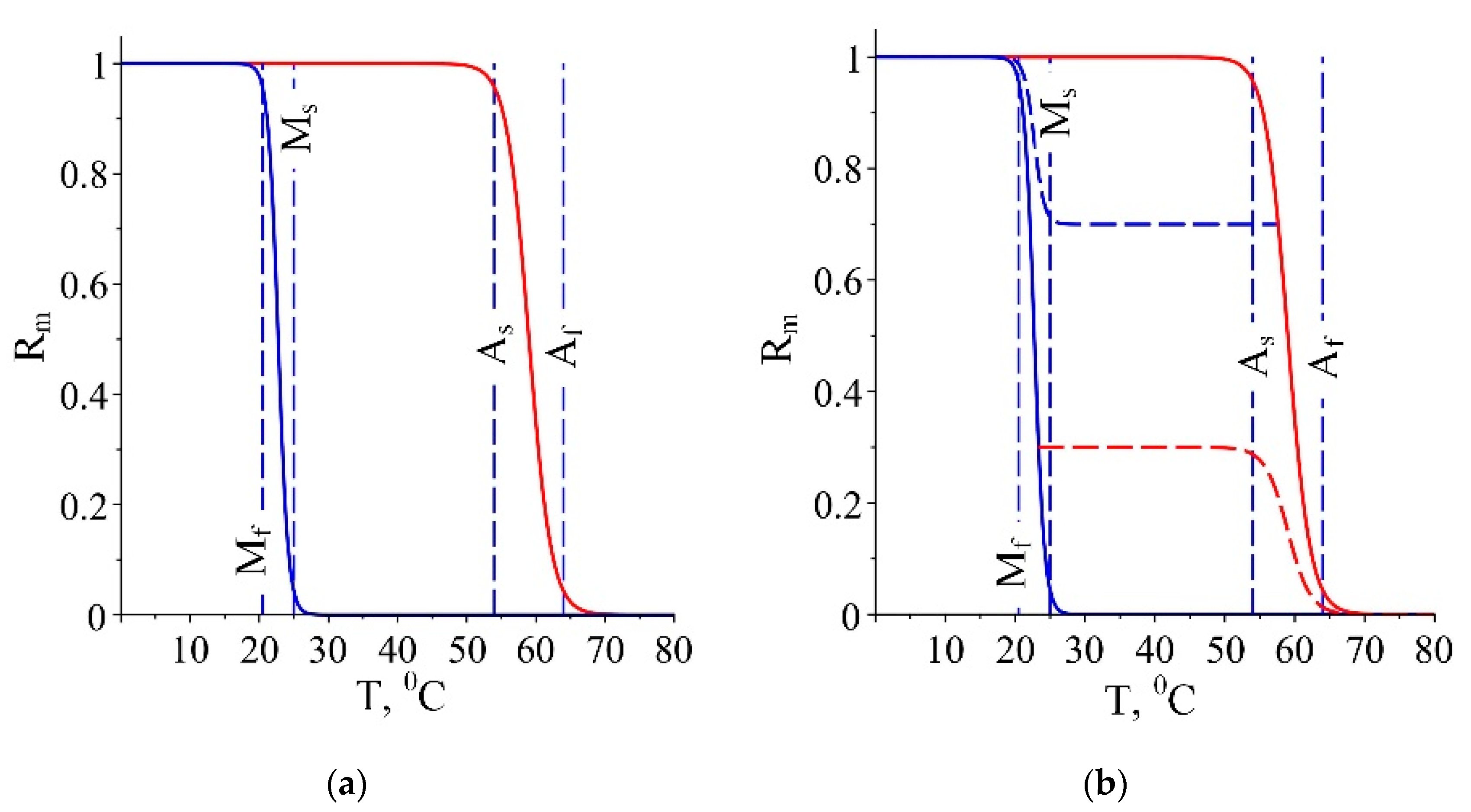
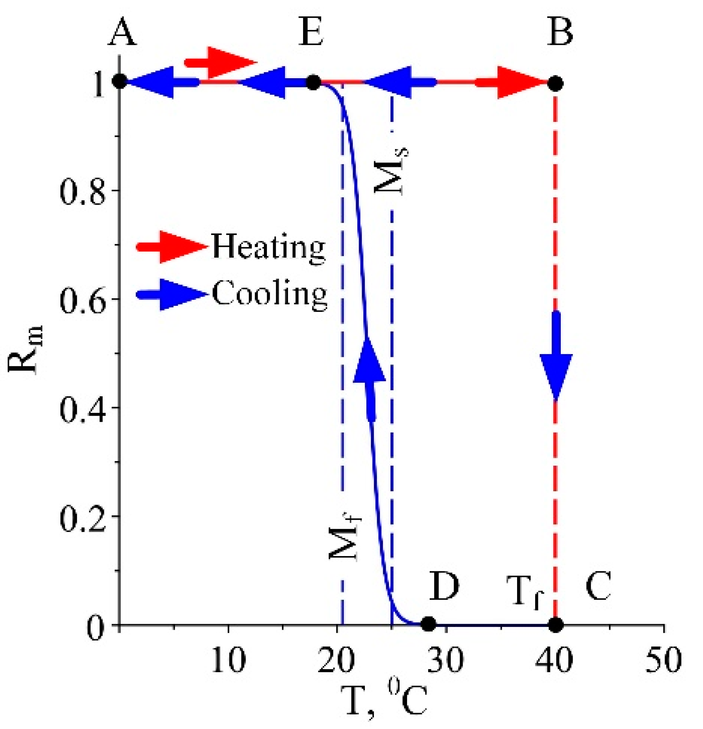
3.2. Mathematical Modelling of the Minor and Sub Minor Hystereses

The hysteresis of the SMA is described using the relative martensitic fraction

$$R_m\left(T\right)=\frac{V_m }{V_s}$$

(35)

where V_m is the volume of the martensite in the total volume vs. of the SMA wire. According to Madill’s model [41]:

$$R_m\left(T\right)=\{\begin{array}{c}{R}_m^C\left(\theta ,t\right), \dot{T}<0 \left(cooling\right)\\ R_m^H\left(\theta ,t\right), \dot{T}>0 \left(heating\right)\end{array}$$

(36)

where

$$R_m^C\left(\theta ,t\right)=\frac{R_{ma}^C\left(t\right)}{1+e^{k_m^C(\theta -{\beta }^C)}}+R_{mb}^C\left(t\right),$$

(37)

$$R_m^H\left(\theta ,t\right)=\frac{R_{ma}^H\left(t\right)}{1+e^{k_m^H(\theta -{\beta }^H)}}+R_{mb}^H\left(t\right),$$

(38)

$\theta =T-T_{\infty }$ is the difference between the current temperature T and the ambient temperature $T_{\infty }$, ${\beta }^{C\left(H\right)}$ is the inflection point temperature defined as

$${\beta }^{C\left(H\right)}=\{\begin{array}{c}{\beta }^C =\frac{1}{2} (M_s+M_f) -T_{\infty }+c_m\left(\sigma -{\sigma }_0\right) , if \dot{T}<0 \\ {\beta }^H= \frac{1}{2} (A_s+A_f) -T_{\infty }+c_m\left(\sigma -{\sigma }_0\right), if \dot{T}>0 \end{array}$$

(39)

where $\sigma$ and σ₀ are the current and tensile stress at $\theta =0$, $k_m^C$, $k_m^H$ referred to as temperature constants of cooling and heating, respectively, and M_s, M_f, A_s, A_f are the start martensite, final martensite, start austenite and final austenite temperatures correspondingly. The functions $R_{ma}^C\left(t\right)$, $R_{mb}^C\left(t\right)$, $R_{ma}^H\left(t\right)$, and remain constant if the wire is just being heated or just being cooled, and changes only if the sign of the fluctuation of the temperature changes.

In the present paper, in contrast to [41], it is assumed that if the fluctuation sign changes during the transition period [M_s, M_f] or [A_f, A_s], the functions depend on the values of the martensite fraction $R_m^f$ and temperature T_f at which the sign of the temperature fluctuation changes. If the sign of the temperature fluctuation changes from positive to negative, i.e., from heating to cooling, then

$$R_{ma}^C=\{\begin{array}{l}1, if M_f>T_f>A_f \\ R_m^f, if A_f\ge T_f\ge A_s \end{array}$$

(40)

$$R_{mb}^C=\{\begin{array}{l}0, if M_f>T_f>A_f \\ 0, if A_f\ge T_f\ge A_s \end{array}$$

(41)

In the opposite case, when the temperature fluctuation sign changes from negative to positive respectively for cooling to heating, the functions are:

$$R_{ma}^H=\{\begin{array}{l}1 -R_m^f, if M_f>T_f>A_f \\ R_m^f, if M_s\ge T_f\ge M_f \end{array}$$

(42)

$$R_{mb}^H=\{\begin{array}{l}0, if M_f>T_f>A_f \\ 1-R_m^f, if M_s\ge T_f\ge M_f \end{array}$$

(43)

Both cases are illustrated in Figure 2.

The same Equations (40)–(43) can be applied if the change of the temperature gradient sign is in the temperature interval [M_s, A_s]. In this case, the hysteresis does not exist, but a jump discontinuity in the point T_f of change of the fluctuation sign of the relative martensite fraction is avoided. In Figure 3, a case is illustrated where a discontinuity is possible. If M_s < T_f < A_s then, after moving from points A to B during heating, a cooling appears at point T_f. If (14) is applied, the cooling process starts from point B, and the jump BC appears, followed by a smooth cooling along the curve DEA.

The behaviour according to the improved model (40)–(43) is presented in Figure 3 by the line BA (blue arrows), which presents a realistic change of the temperature for this case. A similar discontinuous function for R_m can be considered if cooling from a temperature T > A_f is present and for $T_f\in \left[M_s,A_s\right]$ a heating appears.

Sub minor (or sub sub minor) hystereses can appear only in already exited minor (sub minor) hysteresis. The temperature of the beginning of the sub minor hysteresis is denoted by $T_f^s$ and the martensite fraction correspondent to this temperature is denoted as $R_m^{fs}$. The second important condition for the existence of sub minor hysteresis is $M_f<T_f^s<M_s$ for cooling minor hysteresis (Figure 4a) or for heating minor hysteresis $A_s<T_f^s<A_f$ (Figure 4b).

If the point of change the fluctuation sign is in the interval $T_f^s\in \left[M_s,A_s\right]$, the hysteresis degenerates into a straight line, similarly to the case explained in Figure 3. The sub minor hystereses are described with similar formulae to (40)–(43) as follows:

$$R_{ma}^C=\{\begin{array}{l}1, if M_f>T_f^s>A_f \\ R_m^{fs}, if A_f\ge T_f^s\ge A_s \end{array}$$

(44)

$$R_{mb}^C=\{\begin{array}{l}0, if M_f>T_f^s>A_f \\ 0, if A_f\ge T_f^s\ge A_s \end{array}$$

(45)

When the temperature fluctuation sign changes from negative to positive respectively for cooling to heating, the functions are

$$R_{ma}^H=\{\begin{array}{l}{R}_m^f -R_m^{fs}, if M_f>T_f^s>A_f \\ R_m^{fs}, if M_s\ge T_f^s\ge M_f \end{array}$$

(46)

$$R_{mb}^H=\{\begin{array}{l}0 if M_f>T_f^s>A_f \\ 1-R_m^{fc} if M_s\ge T_f^s\ge M_f \end{array}$$

(47)

A numerical experiment is conducted to test the developed algorithm for drawing minor and sub minor hystereses. In Figure 5a, a test function of the temperature is shown as a function of time. It is assumed that the initial temperature T₀ is when the SMA changes from austenite to martensite, i.e., the cooling process is present, and the SMA is in austenite phase.

The temperature fluctuations occur when heating changes with cooling and vice versa. In Figure 5a, these fluctuation points correspond to the local temperature extremums denoted by T_i (i = 1, 2, …, 14). A numerical algorithm for determining the fluctuation points is developed, and the results are depicted in Figure 5b. According to the algorithm, the sign of the temperature derivative as a function of time is calculated by the function $sd{T}_i=sign\dot{T}$ and its values are ±1. An additional function $sdd{T}_i=sd{T}_{i+1}-sd{T}_i$ that successively finds the differences of two adjacent signums of the temperature derivatives indicates that a fluctuation occurs if it obtains a value of ±2. Depending on where the point of the temperature fluctuation is, the appropriate equation for calculating the relative martensitic fraction is applied. The two graphs in Figure 6 show both cases for possible calculations of martensite fraction. If the model (36) is used (Figure 6a) it can be distinguished 10 cases of jump points. The relative martensite fraction is a smooth function only for the points T₁₂ ÷ T₁₄ which lies outside the temperature interval [M_f,A_f]. In Figure 6b, the points obtained using the improved model are shown. As one can see, the degenerated hysteresis loop appears for points T₀ ÷ T₈. Points T₉ and T₁₀ describe a sub minor hysteresis loop, and a minor loop starts from point T₁₁.

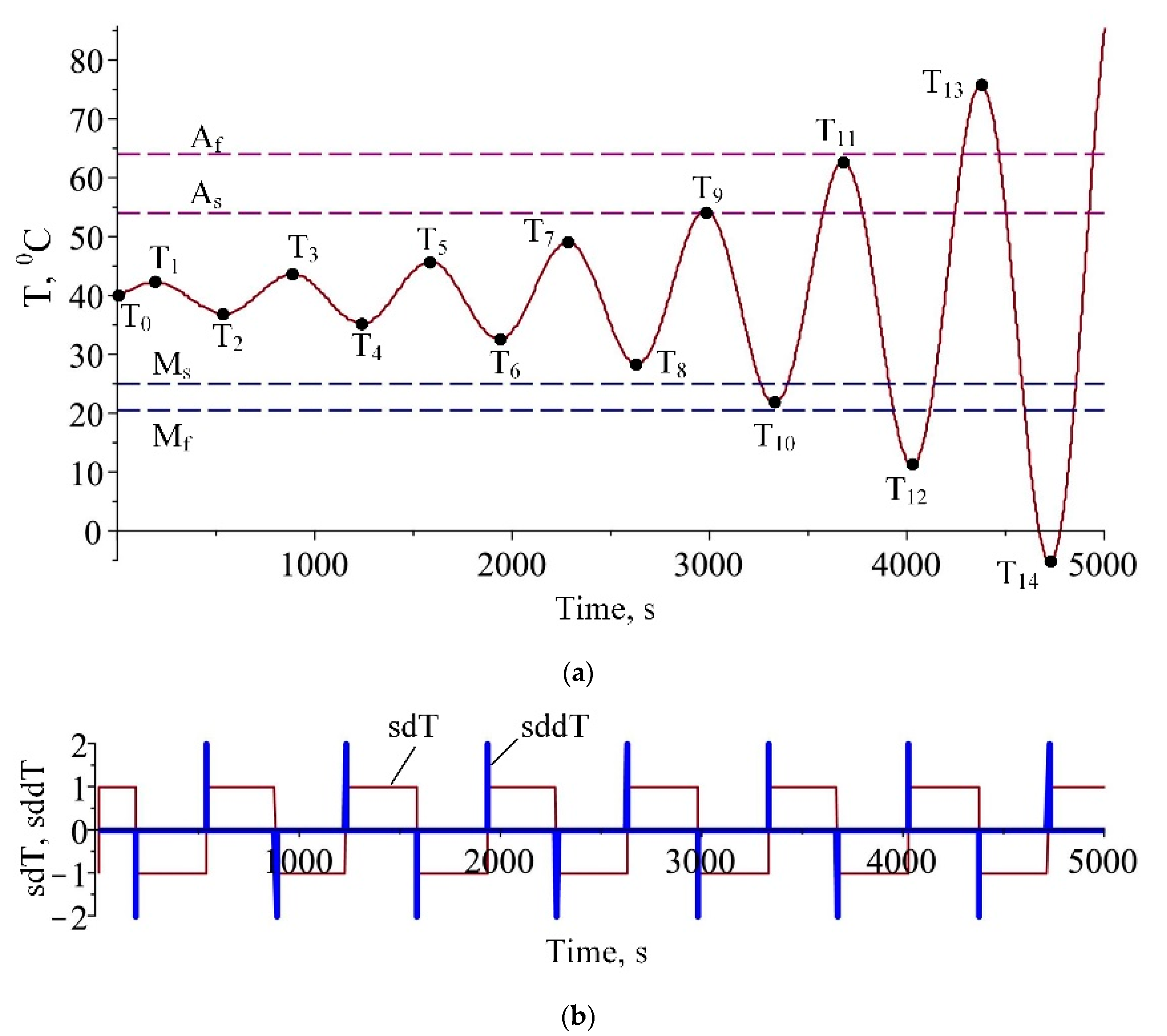
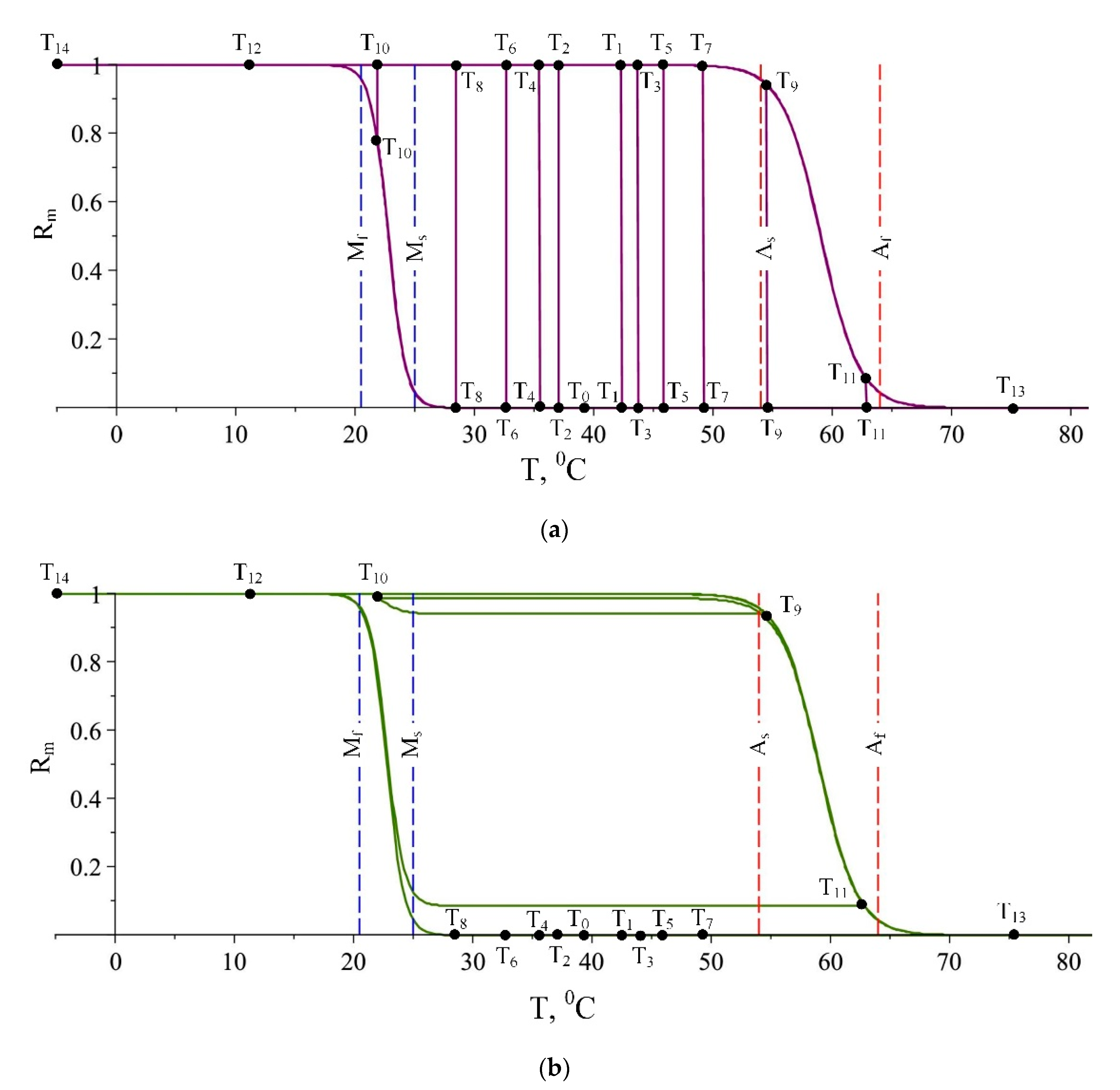
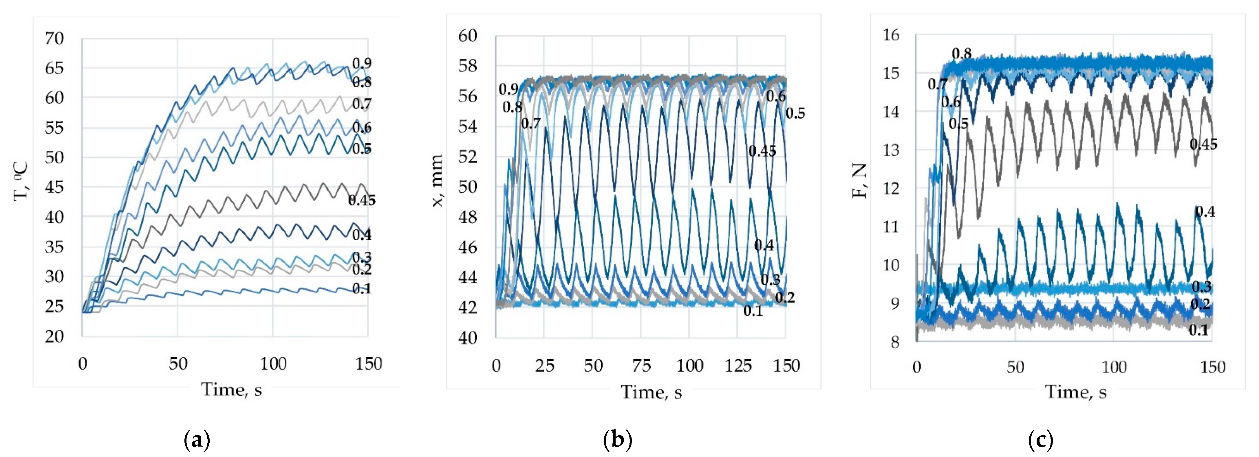
4. Numerical Study of the System Behaviour Using Pulse Width Modulation Control

The thermo-mechanical system behaviour is investigated by conducting numerical experiments under different initial conditions and PWM voltage using the numerical values in

Table 1. Numerical values of the constants.

Parameter	Notation	Value	Unit
Diameter of SMA wire	d	0.00035	m
Initial length of SMA wire	s0	0.160	m
Voltage	u	5	V
Resistance	R	52	Ω
Density of SMA	${\rho }_s$	6450	kg/m3
Specific heat	$c_p$	200	J/(kg·°C)
Convection heat transfer coefficient	$h_c$	70	W/(m2·°C)
Room temperature		26	°C
Martensite Young’s Module	$E_m$	21.7 × 109	Pa
Young’s modulus of NiTi at partly twinned martensite	$E_T$	0.56 × 109	Pa
Young’s modulus of NiTi at detwinned martensite	$E_d$	11.1 × 109	Pa
Austenite Young’s modulus	$E_a$	55.5 × 109	Pa
Yield strain of twined martensite	${\epsilon }_m^y$	0.0024	-
Minimum strain of detwinned martensite	${\epsilon }_m^d$	0.044	-

. For this purpose, the voltage u in (13) is represented as a rectangular pulse waveform:

$$u\left(t\right)=\{\begin{array}{c}\begin{array}{l}0, \mathrm{if} \frac{n+z}{f}\le t\le \frac{n+z+1}{f}\\ u_0, \mathrm{otherwise}\end{array}\end{array}$$

(48)

where u₀ is the amplitude of the rectangular pulse, f is the frequency of the waveform, n = trunc(t × f) is the consecutive number of the period, $0<z<1$ is the duty cycle of the waveform. The function trunc(k) returns the greatest integer less than or equal to k.

Figure 7a shows the graph of the temperature of the SMA wire for a single cycle during the heating (red line) and cooling (blue line), computed according to (13) for PWM frequency f = 0.05 Hz and z = 0.5. As one can see, the heating and cooling are performed at the same speed. Since in the law of variation of temperature, the voltage is of the second degree, the sign of the voltage impulses does not matter, and both positive and negative pulses will affect the temperature in the same way affecting only the amplitude and duration. The graph suggests that the pulse length should be determined depending on the temperature time constant of the thermal subsystem. If the pulse duration is longer than 5τ, the wire temperature reaches ≈98% of its limit value, which means that the use of pulses longer than 5τ is pointless. Therefore, PWM frequency lower than z/5τ is not recommended because the wire temperature will be equal to the limit temperature at a lower frequency and cannot be controlled in practice.

Figure 7b shows the time evolution of the temperature of the wire at a frequency of f = 0.1 Hz, z = 0.5, R = 200 Ω, c_p = 900 J/(kg·°C), h_c = 18 W/(m²·°C). The dashed line (pos.1) depicts the temperature time evolution without using PWM. As can be seen, the temperature reaches its limit value (19). In the same graph, the temperature when PWM is applied is shown (pos.2). The parts of the curve in which the wire is heated are shown in red, and the parts in which the cooling is performed are shown in blue. The limit temperature (19) cannot be reached when PWM is used due to cooling sections depending on duty cycle value. Maximum wire temperature and temperature increasing rates are controlled by changing the duty cycle value, which can improve the control of the actuator, especially in cases where a smoother operation is required. The limited cooling rate is a major factor that limits the actuator’s performance [44].

5. Experimental Studies and Validation of the Model

The experimental studies of the SMA actuator are conducted using an original experimental setup [45,46], shown in Figure 8. Its functionality allows the measurement of the SMA wire’s force, temperature, and displacement as a function of time. The experimental setup design with PWM regulated temperature tests wires with different diameters and lengths, creating different pre-tension forces.

The experimental setup consists of a base 1 with installed a lead screw 2 and a bearing. By rotating the screw, a pre-tension is created in the serially connected spring 3 and the SMA wire 4. One end of the SMA wire is connected to the spring through a magnetic displacement sensor 5, and the other end is connected to sensor 6 for measuring the wire tension force through a lever. Thermocouple 7, connected to the SMA wire, measures its temperature. The sensors register the wire length and temperature change, and the force and their output signals are sent to NI cDAQ 9174 data acquisition system 8. A LabVIEW graphical program 9 for processing and visualization of the data is developed 9.

Figure 9 shows the experimentally obtained graphs for the wire’s temperature, force, and displacements for a duty cycle variation in the range of 0.1 ÷ 0.9 for PWM frequency f = 0.1. Analysis of the presented in Figure 9a results for the temperature show that the increase in the duty cycle value leads to a rise in the temperature of the SMA wire. For every duty cycle value, the rise in the temperature in time is exponential, as suggested by (17). Periodic temperature fluctuations with the frequency of PWM and variable amplitude are present due to the heating and cooling of the wire. A temperature jump is present during the transition from the duty cycle value of 0.4 to 0.5, suggesting a nonlinear relationship. When the duty cycle value increases after 0.8, the temperature does not rise anymore, and the tendency is to be equal to the limit temperature. The displacement and force results, shown in Figure 9b,c correspondingly, have a similar character. The fluctuations of the displacement are maximal at a value 0.4. Increasing the duty cycle value from 0.1 to 0.4 leads to an increase in displacement of about 5 mm. Increasing the duty cycle value to 0.5 results in a jump in the displacement of about 8 mm, and a further increase to 0.9 practically does not causes an increase in the displacement. It can be concluded that a relatively accurate displacement with a small amplitude of fluctuations by changing the duty cycle value can only be maintained in the range of very low (0.1 ÷ 0.2) or very high (0.7 ÷ 0.9) values of the duty cycle, with the corresponding displacement of 42 mm and 57 mm. Stable constant intermediate displacement values were impossible to obtain by setting a constant duty cycle value. Similar conclusions can be made about the SMA wire force—by changing the duty cycle value, it is possible to obtain constant values of the SMA force about 9 N or about 15 N. Figure 10 and Figure 11 show similar graphs for PWM frequency values equal to 1 Hz and 10 Hz correspondingly. As one can see, the amplitudes of fluctuations are very small, and the laws of change of the temperature, displacement and force are similar to the already discussed graphs in Figure 9.

In Figure 12, the change in temperature, displacement and force for duty cycle value of z = 0.5 and different PWM frequencies—from 0.01 Hz to 0.4 Hz—are shown. Each graph is labelled with the PWM frequency at which the corresponding graph is obtained. At a frequency of 0.01 Hz, the exponential nature of the wire temperature during heating and cooling is visible. At all frequencies, there are fluctuations in the temperature, and with the increase in the frequency, the amplitude of the fluctuations decreases. For all cases, the average temperature is about 43 °C, indicating that this average temperature can be maintained at any frequency but with varying degrees of deviation due to the periodic fluctuations. In the same figure, the corresponding graphs of the displacement are shown. At a frequency of 0.01 Hz, the average displacement value is 50 mm, and its variation is between 42 and 57 mm. At a frequency of 0.1 Hz, the displacement variation is much smaller, but the average displacement value is about 55 mm. The graph for the force has a similar character.

The validation of the developed mathematical model (13) is performed by comparing numerical and experimentally obtained results. Figure 13a shows theoretical and experimental results for the temperature and displacement for duty cycle value 0.5 and PWM frequency equal to 0.01 Hz. By positions 1 and 3, the theoretical values of the temperature and displacement correspondingly, computed using the system (13) are denoted. By positions 2 and 4, the experimental values of the temperature and displacement correspondingly are denoted. Analysis of the similarity of the graphs shows an accurate enough degree of coincidence. This is also confirmed by the hysteresis shown in Figure 13b, in which the double loop shows differences for the two illustrated cycles. The differences between the graphs can be explained by insufficiently accurate identification of the numerical values of the parameters, as well as by the significant sensitivity of the system to some factors not included in the mathematical model or whose influence cannot be predicted, mainly—the presence of random airflows, imperfections in the design of the experimental setup and constantly changing environmental conditions during the experiment. The influence of the thermocouple on the temperature measured is minimized using a thermocouple whose dimensions are close to the diameter of the wire [47].

6. Conclusions

This paper presented the development of a mathematical model of an actuator consisting of shape memory alloy wire connected in series with bias spring, allowing modelling in-depth of the actuator dynamics. The model considers the dynamics of the mechanical subsystem of the actuator and the heat exchange between the wire and the environment. Through a detailed theoretical analysis, two nonlinear ordinary differential equations were obtained, the generalized coordinates of which are the displacement of the mass representing the actuator and the temperature of the wire. Further analysis shows that the stiffness coefficient of the wire and the natural frequency of the mechanical subsystem depends on the temperature and the deformation of the wire. It is concluded that the pulse length of the control voltage signal should be determined depending on the time constant of the system, and the use of pulses longer than 5τ is pointless.

To increase the accuracy of the modelling, in the present work an algorithm for modelling the minor and sub minor hystereses has been developed, which eliminates the shortcomings of the classical model, especially the jumps in the martensitic fraction. This algorithm increases modelling accuracy, especially when using PWM control, for which minor and sub minor hystereses are likely to occur.

Experimental studies show that the system is very sensitive, and there are factors whose presence cannot be considered in the mathematical model. Experiments have shown that increasing the duty cycle increases the temperature of the SMA wire, but a linear relationship does not describe this increase. The fact that by setting constant values of the duty cycle is not possible to obtain a stable value of displacement and force shows that it is more appropriate to use a feedback control system in which such factors as voltage, frequency and duty cycle can serve as control inputs. The validation of the model shows that the differences between the results of the developed model and the experimental results are acceptable.

The derived dynamic equations increase the accuracy of mathematical modelling and serve as a basis for designing such actuators and creating an improved automatic feedback control system to maintain a given displacement (force) or trajectory tracking.

References

1. Jani, J.M.; Leary, M.; Subic, A.; Gibson, M.A. A review of shape memory alloy research, applications and opportunities. Mater. Des. 2014, 56, 1078–1113. [Google Scholar] [CrossRef]
2. Todorov, T.; Mitrev, R.; Penev, I. Force analysis and kinematic optimization of a fluid valve driven by shape memory alloys. Rep. Mech. Eng. 2020, 1, 61–76. [Google Scholar] [CrossRef]
3. Petrini, L.; Migliavacca, F. Biomedical Applications of Shape Memory Alloys. J. Metall. 2011, 2011, 501483. [Google Scholar] [CrossRef]
4. Anjum, N.; He, J.; Ain, Q.; Tian, D. Li-He’s modified homotopy perturbation method for doubly-clamped electrically actuated microbeams-based microelectromechanical system. Facta Univ.-Ser. Mech. Eng. 2021, in press. [Google Scholar] [CrossRef]
5. Noll, M.-U.; Lentz, L.; von Wagner, U. On the discretization of a bistable cantilever beam with application to energy harvesting. Facta Univ.-Ser. Mech. Eng. 2019, 17, 125–139. [Google Scholar] [CrossRef]
6. Marinković, D.; Rama, G.; Zehn, M. Abaqus implementation of a corotational piezoelectric 3-node shell element with drilling degree of freedom. Facta Univ.-Ser. Mech. Eng. 2019, 17, 269–283. [Google Scholar] [CrossRef] [Green Version]
7. Tanaka, K.A. Thermomechanical sketch of shape memory effect: One-dimensional tensile behavior. Res. Mech. 1986, 18, 251–263. [Google Scholar]
8. Liang, C.; Rogers, C.A. One-dimensional thermomechanical constitutive relations for shape memory material. J. Intell. Mater. Syst. Struct. 1990, 1, 207–234. [Google Scholar] [CrossRef]
9. Brinson, L.C. One dimensional constitutive behavior of shape memory alloys: Thermomechanical derivation with nonconstant material functions and redefined martensite internal variable. J. Intell. Mater. Syst. Struct. 1993, 4, 229–242. [Google Scholar] [CrossRef]
10. Sayyaadi, H.; Zakerzadeh, M.R.; Salehi, H. A comparative analysis of some one-dimensional shape memory alloy constitutive models based on experimental tests. Sci. Iran. 2012, 19, 249–257. [Google Scholar] [CrossRef] [Green Version]
11. Achenbach, M. A model for an alloy with shape memory. Int. J. Plast. 1989, 5, 371–395. [Google Scholar] [CrossRef]
12. Seelecke, S.; Müller, I. Shape memory alloy actuators in smart structures: Modeling and simulation. Appl. Mech. Rev. 2004, 57, 23–46. [Google Scholar] [CrossRef]
13. Roh, J.-H. Thermomechanical Modeling of Shape Memory Alloys with Rate Dependency on the Pseudoelastic Behavior. Math. Probl. Eng. 2014, 2014, 204165. [Google Scholar] [CrossRef]
14. Kurzawa, M.; Stachowiak, D. Investigation on thermo-mechanical behavior of shape memory alloy actuator. Arch. Electr. Eng. 2017, 66, 751–760. [Google Scholar] [CrossRef]
15. Sedlák, P.; Frost, M.; Benešová, B.; Ben Zineb, T.; Šittner, P. Thermomechanical model for NiTi-based shape memory alloys including R-phase and material anisotropy under multi-axial loadings. Int. J. Plast. 2012, 39, 132–151. [Google Scholar] [CrossRef]
16. Tanaka, K.; Nishimura, F.; Tobushi, H. Phenomenological Analysis on Subloops in Shape Memory Alloys Due to Incomplete Transformations. J. Intell. Mater. Syst. Struct. 1994, 5, 487–493. [Google Scholar] [CrossRef]
17. Segui, C.; Cesari, E.; Pons, J. Phenomenological modelling of the hysteresis loop in thermoelastic martensitic transformations. Mater. Trans. 1992, 33, 650–658. [Google Scholar]
18. Liu, M.; Hao, L.; Zhang, W.; Zhao, Z. A novel design of shape-memory alloy-based soft robotic gripper with variable stiffness. Int. J. Adv. Robot. Syst. 2020, 17, 172988142090781. [Google Scholar] [CrossRef]
19. Manfredi, L.; Huan, Y.; Cuschieri, A. Low power consumption mini rotary actuator with SMA wires. Smart Mater. Struct. 2017, 26, 115003. [Google Scholar] [CrossRef]
20. Abuzied, H.; Abbas, A.; Awad, M.; Senbel, H. Usage of shape memory alloy actuators for large force active disassembly applications. Heliyon 2020, 6, e04611. [Google Scholar] [CrossRef]
21. Chaitanya, S.K.; Dhanalakshmi, K. Control of Shape Memory Alloy Actuated Gripper using Pulse-Width Modulation. IFAC Proc. Vol. 2014, 47, 408–413. [Google Scholar] [CrossRef]
22. Soother, D.K.; Daudpoto, J.; Chowdhry, B.S. Challenges for practical applications of shape memory alloy actuators. Mater. Res. Express 2020, 7, 073001. [Google Scholar] [CrossRef]
23. Prechtl, J.; Seelecke, S.; Motzki, P.; Rizzello, G. Self-Sensing Control of Antagonistic SMA Actuators Based on Resistance-Displacement Hysteresis Compensation. In Proceedings of the ASME 2020 Conference on Smart Materials, Adaptive Structures and Intelligent Systems, Virtual, Online, 15 September 2020. [Google Scholar] [CrossRef]
24. Ujihara, M.; Carman, G.; Lee, D. Thermal energy harvesting device using ferromagnetic materials. Appl. Phys. Lett. 2007, 91, 093508. [Google Scholar] [CrossRef]
25. Elahinia, M.; Esfahani, E.; Wang, S. Properties and Applications Control of SMA Systems: Review of the State of the Art Shape Memory Alloys: Manufacture, Properties and Applications; Nova Science Publishers: Hauppauge, NY, USA, 2010; pp. 49–68. [Google Scholar]
26. Featherstone, R.; Teh, Y.H. Improving the speed of shape memory alloy actuators by faster electrical heating. In Experimental Robotics IX; Springer: Berlin/Heidelberg, Germany, 2006; pp. 67–76. [Google Scholar]
27. Dynalloy, Inc. Technical Characteristics of Flexinol Actuator Wire; Dynalloy, Inc.: Irvine, CA, USA, 2018; Available online: https://www.dynalloy.com/pdfs/TCF1140.pdf (accessed on 1 September 2021).
28. Villoslada, A.; Escudero, N.; Martín, F.; Flores, A.; Rivera, C.; Collado, M.; Moreno, L. Position control of a shape memory alloy actuator using a four-term bilinear PID controller. Sens. Actuator A Phys. 2015, 236, 257–272. [Google Scholar] [CrossRef] [Green Version]
29. Kha, N.B.; Ahn, K.K. Position Control of Shape Memory Alloy Actuators by Using Self Tuning Fuzzy PID Controller. In Proceedings of the 2006 1ST IEEE Conference on Industrial Electronics and Applications, Singapore, 24–26 May 2006; pp. 1–5. [Google Scholar]
30. Samadi, S.; Koma, A.Y.; Zakerzadeh, M.R.; Heravi, F.N. Control an SMA-actuated rotary actuator by fractional order PID controller. In Proceedings of the 5th RSI International Conference on Robotics and Mechatronics (ICRoM), Tehran, Iran, 25–27 October 2017. [Google Scholar]
31. Ma, N.; Song, G. Control of shape memory alloy actuator using pulse width modulation. Smart Mater. Struct. 2003, 12, 12712. [Google Scholar] [CrossRef] [Green Version]
32. Kim, M.; Shin, Y.J.; Lee, J.Y.; Chu, W.S.; Ahn, S.H. Pulse width modulation as energy-saving strategy of shape memory alloy based smart soft composite actuator. Int. J. Precis. Eng. Manuf. 2017, 18, 895–901. [Google Scholar] [CrossRef]
33. Motzki, P.; Gorges, T.; Kappel, M.; Schmidt, M.; Rizzello, G.; Seelecke, S. High-speed and high-efficiency shape memory alloy actuation. Smart Mater. Struct. 2018, 27, 075047. [Google Scholar] [CrossRef]
34. Price, A.D.; Jnifene, A.; Naguib, H.E. Design and control of a shape memory alloy based dexterous robot hand. Smart Mater. Struct. 2007, 16, 1401. [Google Scholar] [CrossRef]
35. Pan, C.H.; Wang, Y.B.; Pan, H.Y. Development of dynamically artificial flowers driven by shape memory alloy and pulse width modulation. In Proceedings of the 2015 IEEE International Workshop on Advanced Robotics and Its Social Impacts (ARSO), Lyon, France, 30 June–2 July 2015; pp. 1–6. [Google Scholar]
36. Song, G.; Ma, N. Control of Shape Memory Alloy Actuators Using Pulse-Width Pulse-Frequency (PWPF) Modulation. J. Intell. Mater. Syst. Struct. 2003, 14, 15–22. [Google Scholar] [CrossRef]
37. Song, H.; Kubica, E.; Gorbet, R. Resistance modelling of SMA wire actuators. In Proceedings of the International Workshop Smart Materials, Structures & NDT in Aerospace, Montreal, QC, Canada, 2–4 November 2011. [Google Scholar]
38. Sittner, P.; Dayananda, G.N.; Brz-Fernandes, F.M.; Mahesh, K.K.; Novak, V. Electric resistance variation of NiTi shape memory alloy wires in thermomechanical tests: Experiments and simulation. Mater. Sci. Eng. 2008, 481–482, 127–133. [Google Scholar]
39. Talebi, H.; Golestanian, H.; Zakerzadeh, M.R.; Homaei, H. Thermoelectric Heat Transfer Modeling of Shape Memory Alloy Actuators. In Proceedings of the 22st Annual International Conference on Mechanical Engineering-ISME2014, Ahvaz, Iran, 22–24 April 2014; Shahid Chamran University: Ahvaz, Iran, 2014. ISME2014-2206. [Google Scholar]
40. Ikuta, K.; Tsukamoto, M.; Hirose, S. Mathematical model and experimental verification of shape memory alloy for designing micro actuator. In Proceedings of the 1991 IEEE Micro Electro Mechanical Systems, Nara, Japan, 30 January–2 February 1991; pp. 103–108. [Google Scholar]
41. Madill, D.R.; David, W. Modeling and L2-Stability of a Shape Memory Alloy Position Control System. IEEE Trans. Control Syst. Technol. 1998, 6, 473–481. [Google Scholar] [CrossRef]
42. Mitrev, R.; Todorov, T.; Fursov, A.; Fomichev, V.; Il’in, A. A Case Study of Combined Application of Smart Materials in a Thermal Energy Harvester with Vibrating Action. J. Appl. Comput. 2021, 7, 327–381. [Google Scholar]
43. Todorov, T.S.; Fursov, A.S.; Mitrev, R.P.; Fomichev, V.V.; Valtchev, S.; Il’in, A.V. Energy Harvesting with Thermally Induced Vibrations in Shape Memory Alloys by a Constant Temperature Heater. IEEE/ASME Trans. Mechatron. 2021. [Google Scholar] [CrossRef]
44. Nizamani, A.M.; Daudpoto, J.; Nizamani, M.A. Development of Faster SMA Actuators Shape Memory Alloys–Fundamentals and Applications; IntechOpen: London, UK, 2017; pp. 105–126. [Google Scholar]
45. Mitrev, R.P.; Todorov, T.S. A Case Study of Experimental Evaluation of the Parameters of Shape Memory Alloy Wires. In Proceedings of the 10th International Scientific Conference on Engineering, Technologies and Systems, TechSys 2021, Plovdiv, Bulgaria, 27–29 May 2021. in press. [Google Scholar]
46. Ralev, Y.; Todorov, T. Experimental setup for testing shape memory alloys. Bulg. J. Eng. Des. 2015, 27, 5–9. [Google Scholar]
47. Szykowny, S.; Elahinia, M.H. Heat transfer analysis of shape memory alloy actuators. In Proceedings of the IMECE2006, ASME International Mechanical Engineering Congress and Exposition, Chicago, IL, USA, 5–10 November 2006. [Google Scholar]
Figure 1. Schematic diagram of the SMA actuator: 1—SMA wire, 2—bias spring, 3—point mass, 4—force-deformation diagram of the spring, 5—force—deformation diagram of the wire in the austenitic state, 6—force—deformation diagram of the wire in the martensitic state, Fsp—spring force, Fd—damping force, Fs—SMA wire force.
Crystals 11 01120 g001
Figure 2. Diagram of relative martensitic fraction Rm vs. temperature T: (a) Major hysteresis if the sign of the temperature fluctuation changes when Mf > T > Af; (b) Minor hystereses if the change of the sign of the temperature fluctuation is between Mf and Ms or As and Af.
Crystals 11 01120 g002
Figure 3. A jump discontinuity in the martensite fraction when the change of the sign of the temperature fluctuation is in the interval [Ms, As].
Crystals 11 01120 g003
Figure 4. Subminor hystereses: (a) for minor cooling hysteresis; (b) for minor heating hysteresis.
Crystals 11 01120 g004
Figure 5. Graph of the test function: (a) graph of the temperature; (b) temperature indicators sdT and sddT.
Crystals 11 01120 g005
Figure 6. Calculated relative martensitic fraction Rm: (a) The case without considering the minor and sub minor loops; (b) The case with minor and sub minor loops.
Crystals 11 01120 g006
Figure 7. Time evolution of the SMA wire temperature: (a) at f = 0.05 Hz, z = 0.5; (b) at f = 0.1 Hz, z = 0.5.
Crystals 11 01120 g007
Figure 8. Experimental setup for testing the SMA wires.
Crystals 11 01120 g008
Figure 9. Parametric study of the temperature T (a), displacement x (b) and SMA force F (c) for change of duty cycle from 0.1 to 0.9 and f = 0.1 Hz.
Crystals 11 01120 g009
Figure 10. Parametric study of the temperature T (a), displacement x (b) and SMA force F (c) for change of duty cycle from 0.1 to 0.7 and f = 1 Hz.
Crystals 11 01120 g010
Figure 11. Parametric study of the temperature T (a), displacement x (b) and SMA force F (c) for change of duty cycle from 0.1 to 0.7 and f = 10 Hz.
Crystals 11 01120 g011
Figure 12. Parametric study of the temperature T (a), displacement x (b) and SMA force F (c) for different frequencies and z = 0.5.
Crystals 11 01120 g012
Figure 13. Comparison of experimental and numerical results: (a) time evolution of the displacement x and temperature T of the wire; (b) temperature hysteresis.
Crystals 11 01120 g013