
Heterogeneous Ice Growth in Micron-Sized Water Droplets Due to Spontaneous Freezing

 ,
,  , , and
Abstract
:
1. Introduction
2. Methods
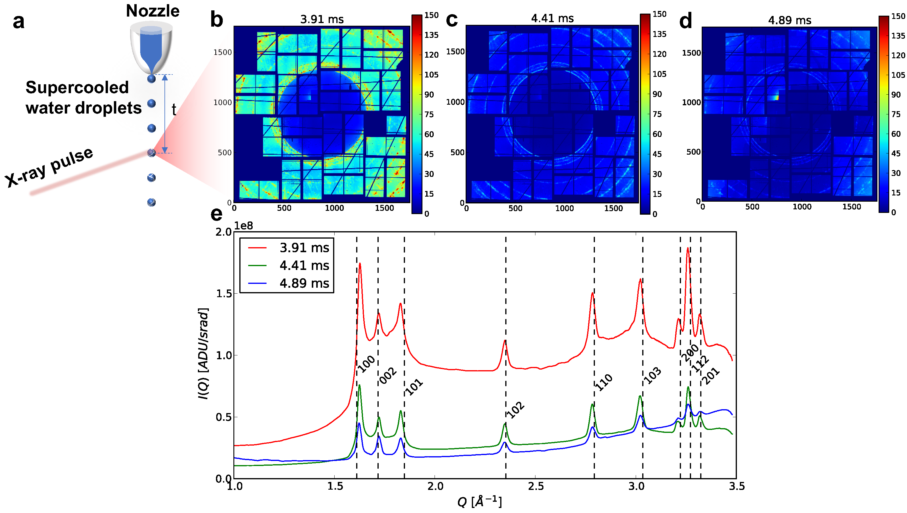
2.1. Experiment
2.2. Data Analysis
2.2.1. Shot Selection
2.2.2. Ensemble Averaging and Data Segmentation
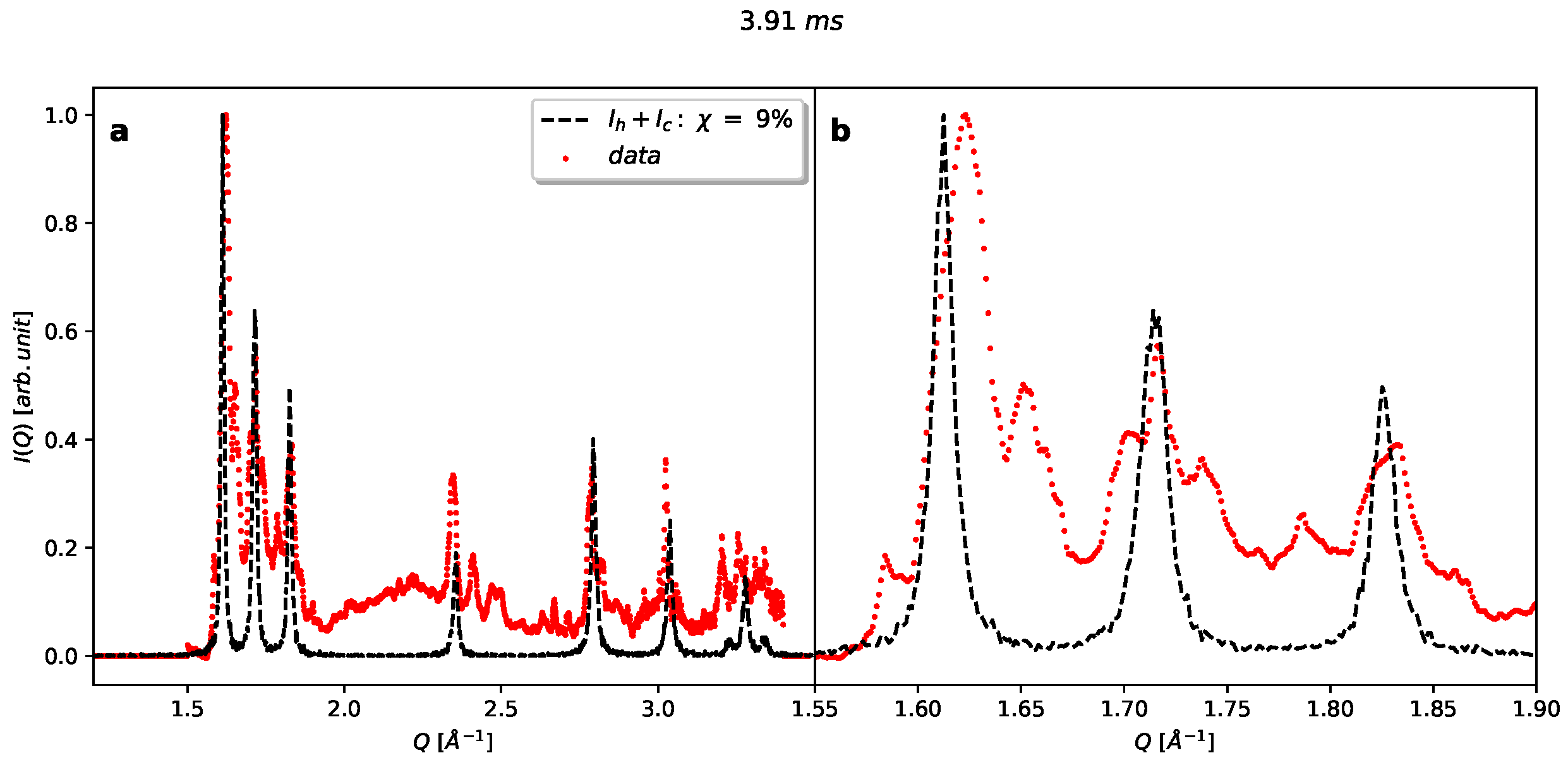
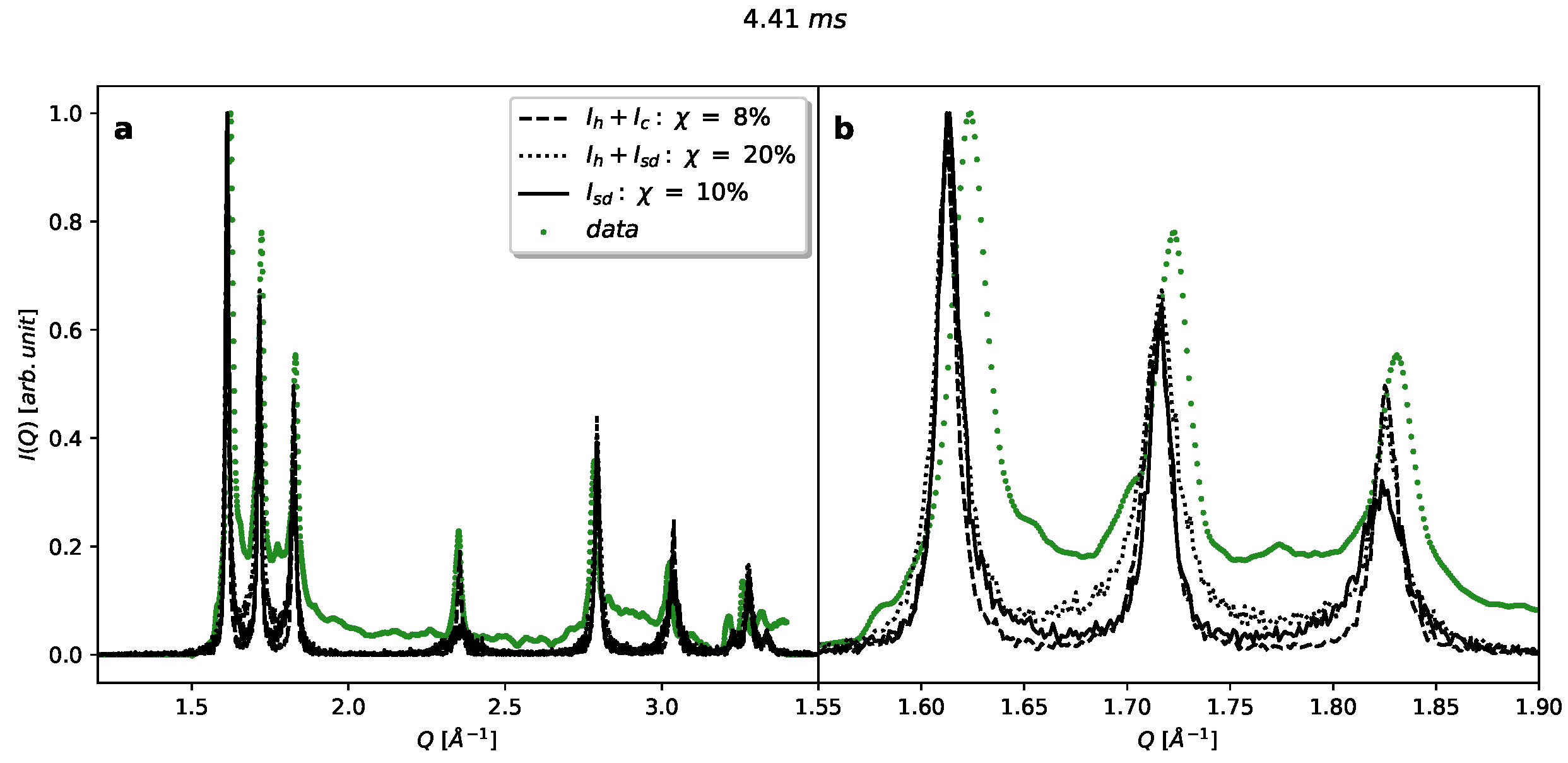
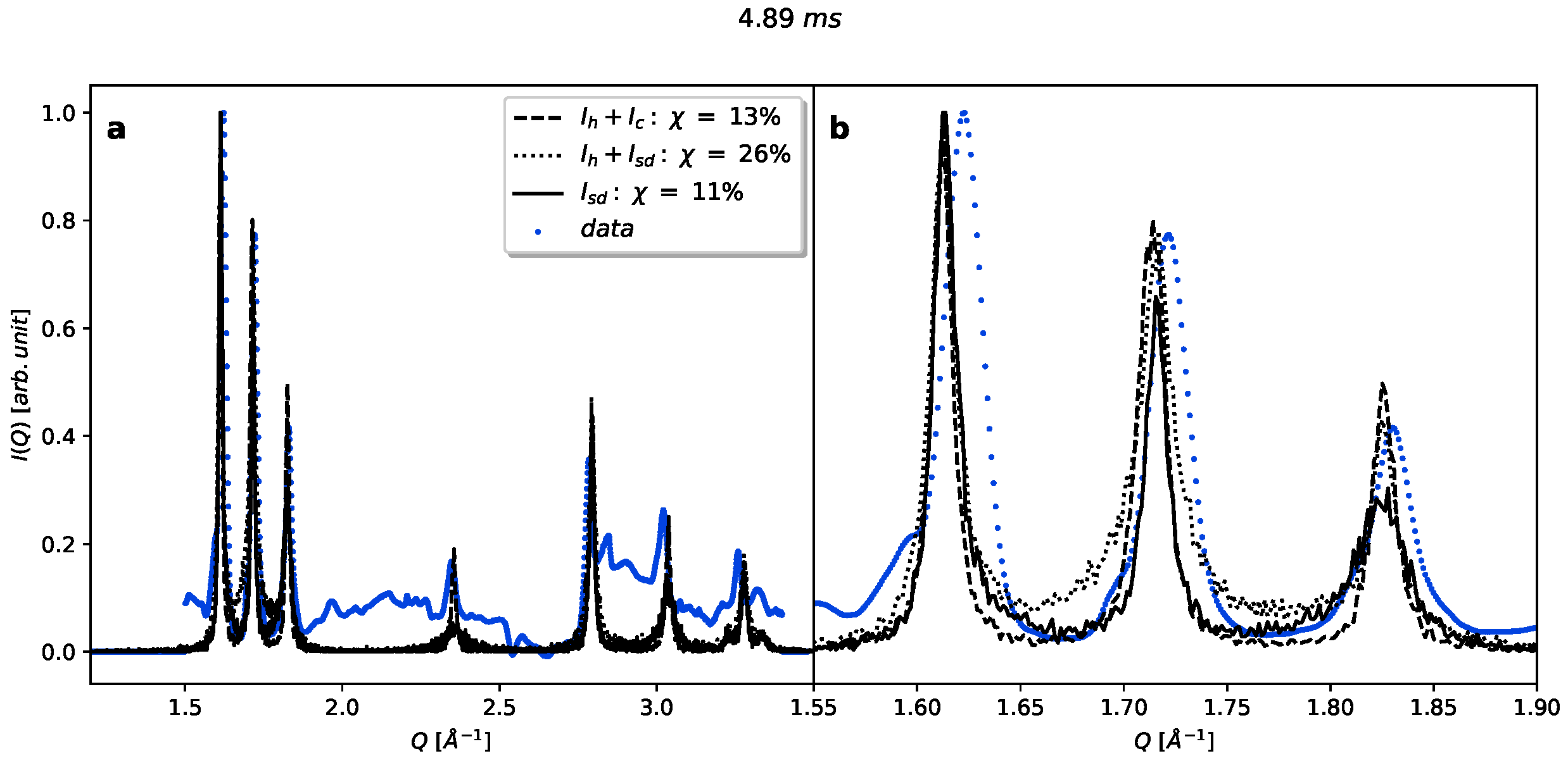
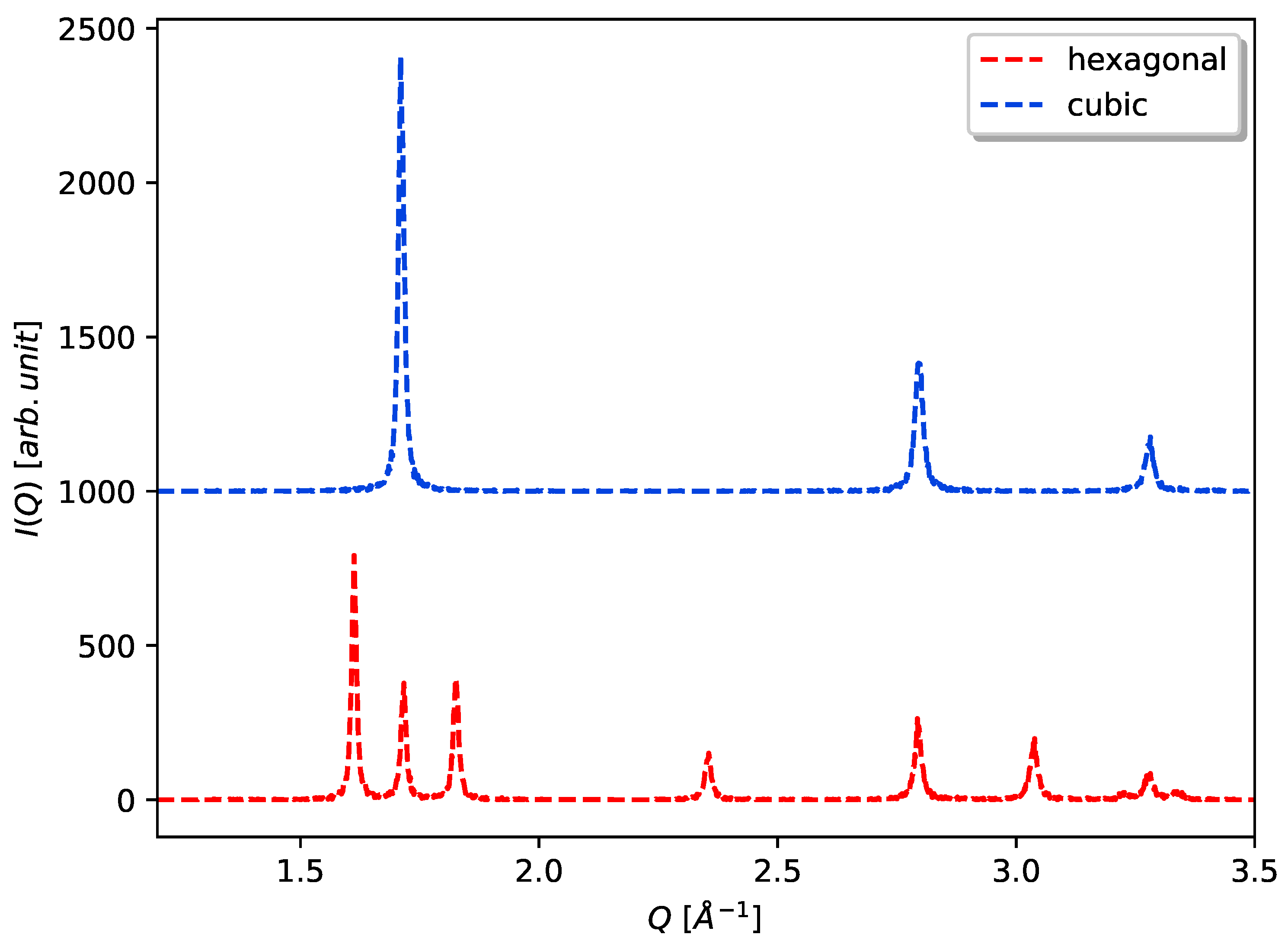
2.2.3. Phase Composition and Cubicity
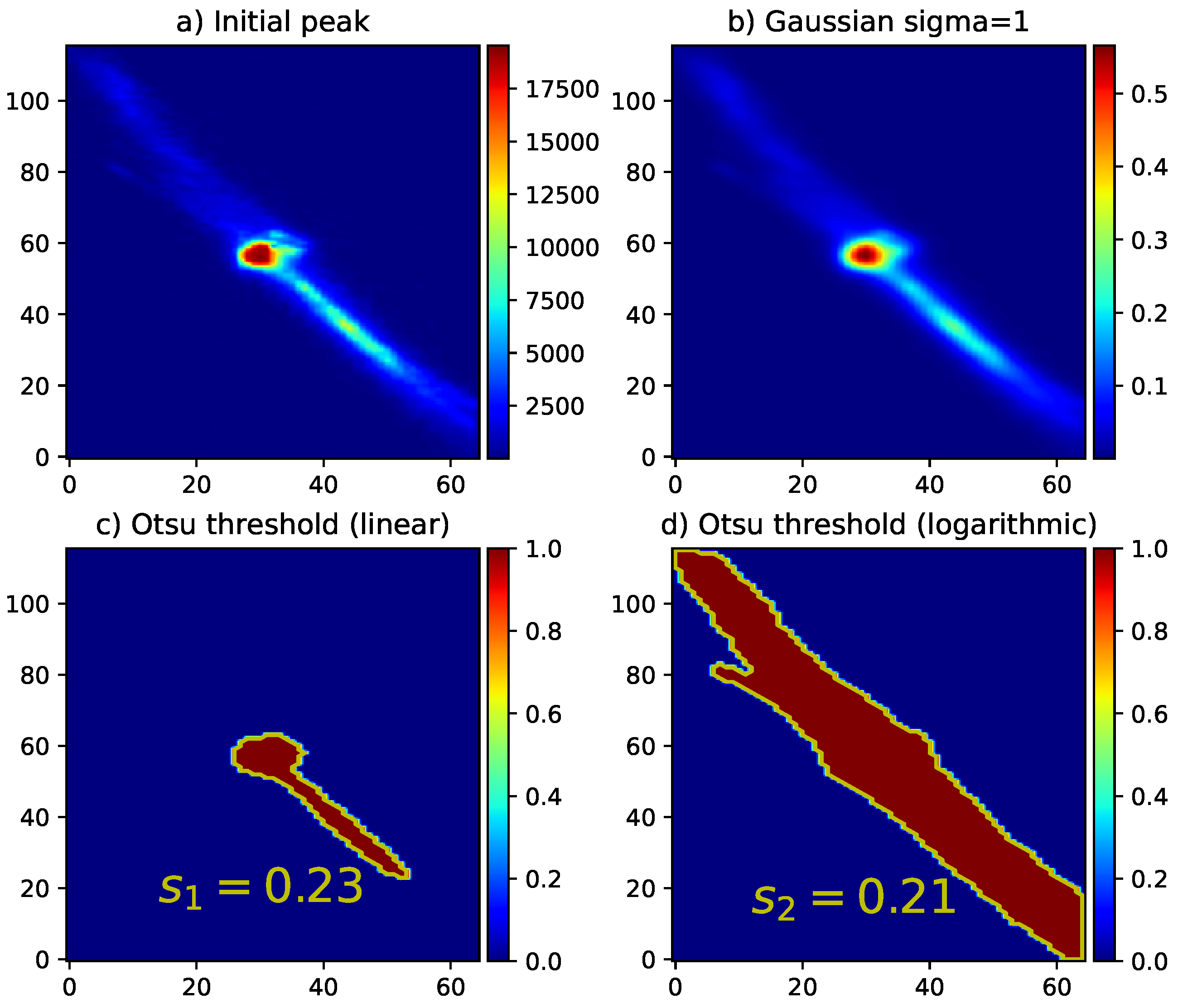
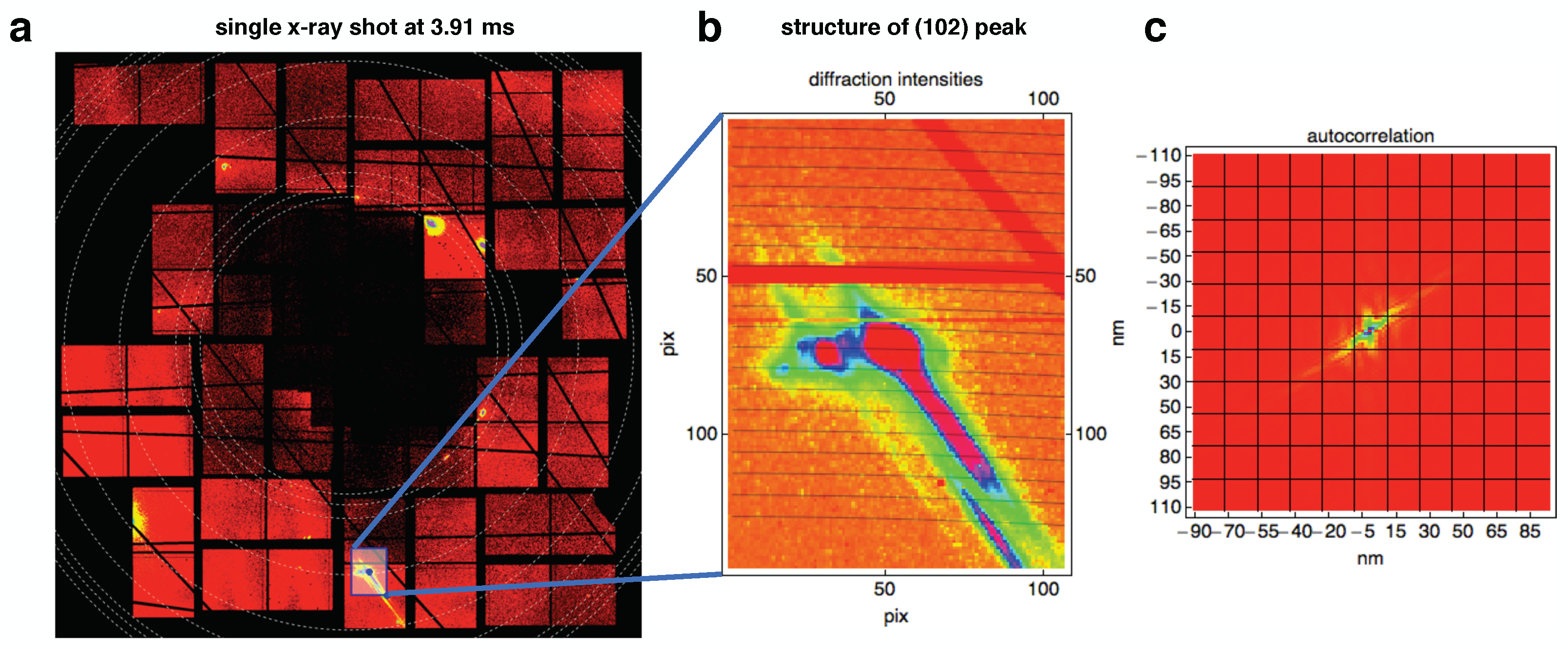
2.2.4. Image Segmentation and Peak Finding
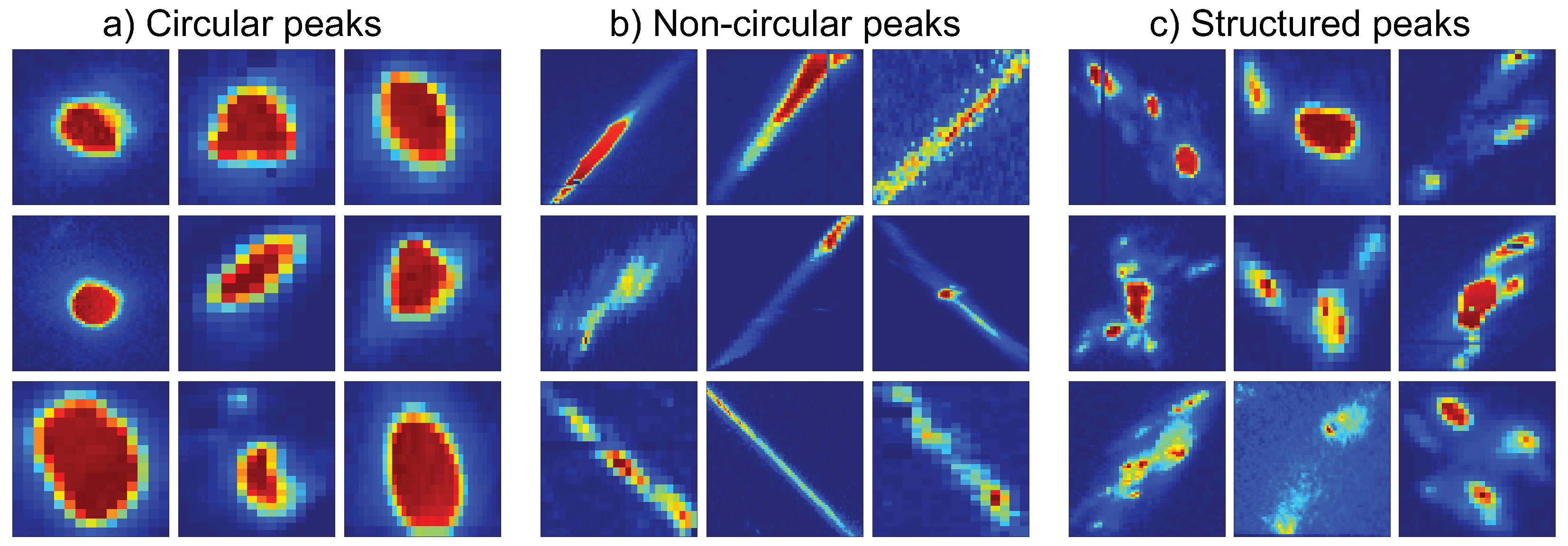
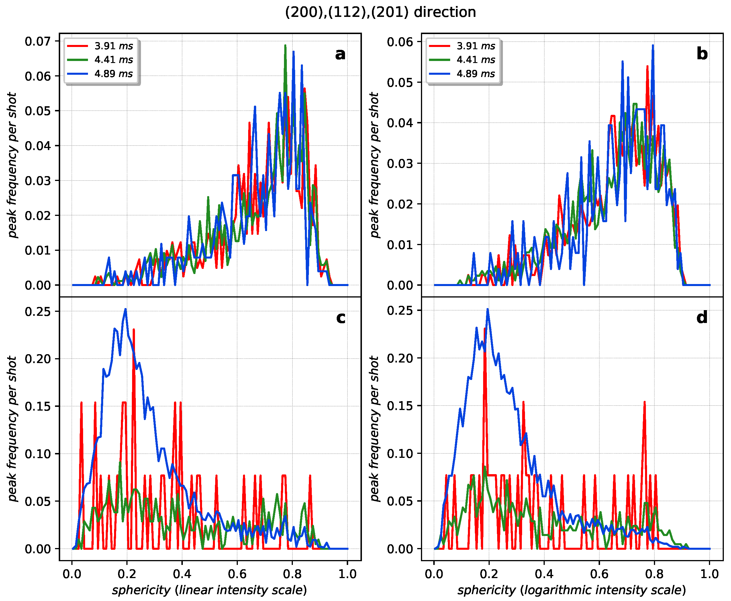
2.2.5. Peak Center of Mass and Sphericity
3. Results
4. Discussion
5. Conclusions
Author Contributions
Funding
Institutional Review Board Statement
Informed Consent Statement
Data Availability Statement
Acknowledgments
Conflicts of Interest
Appendix A
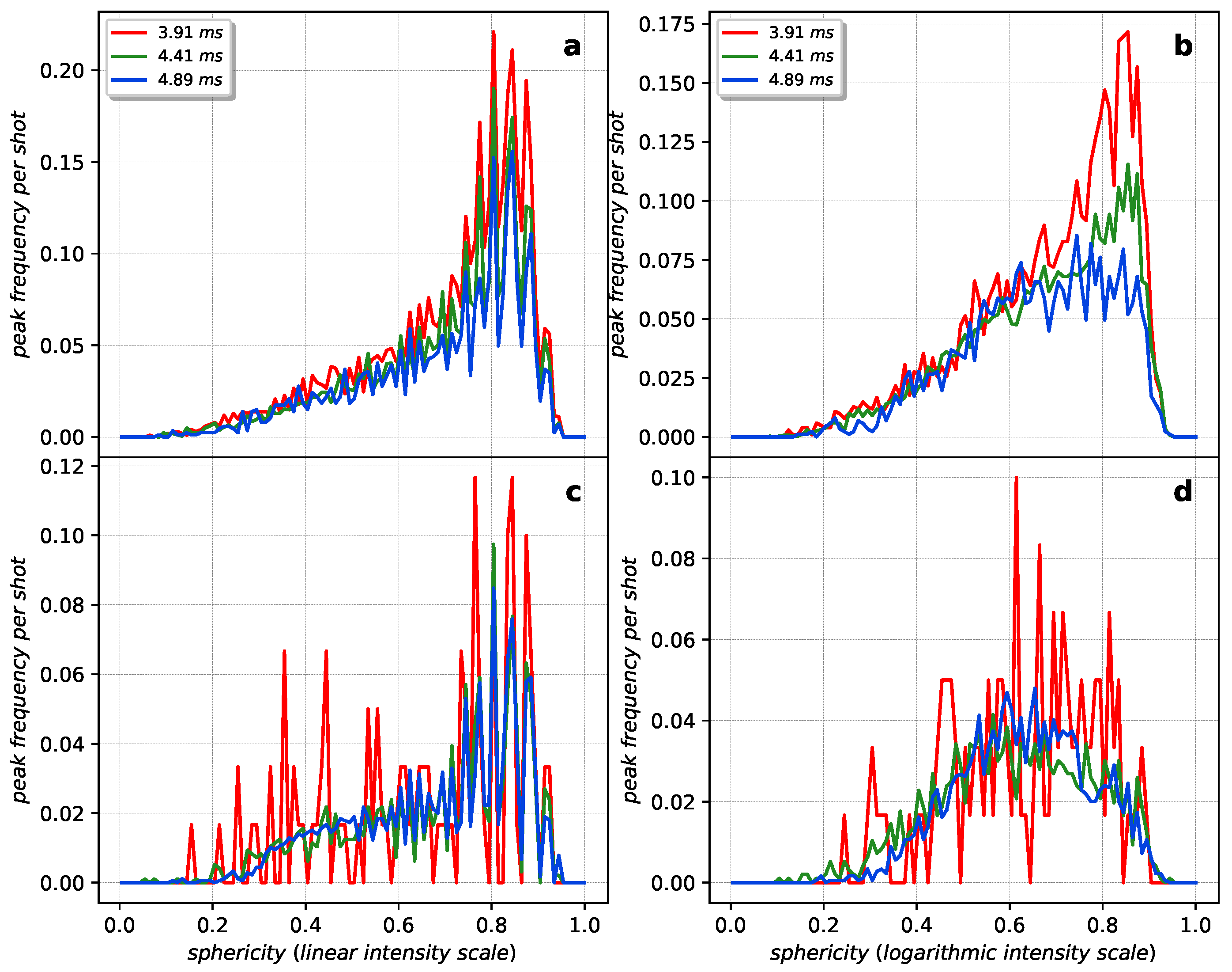
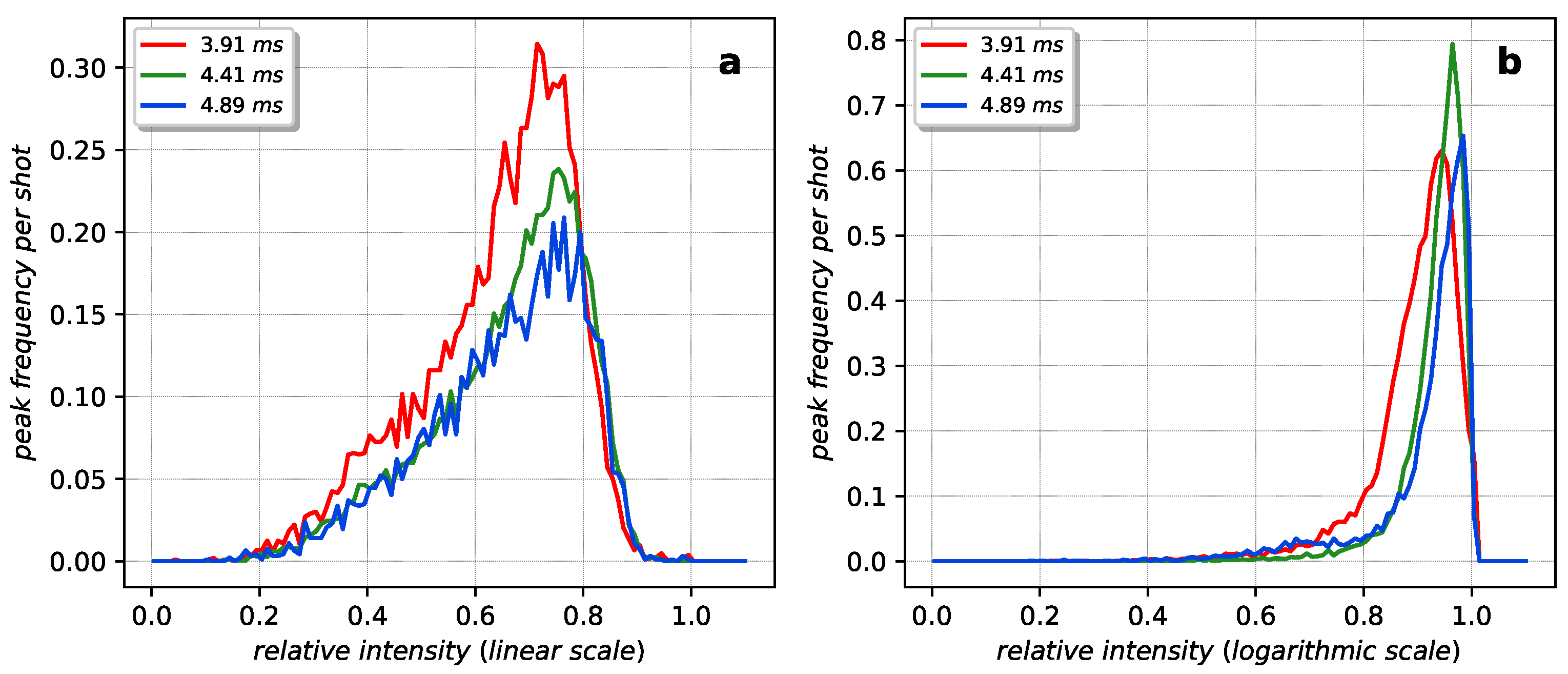
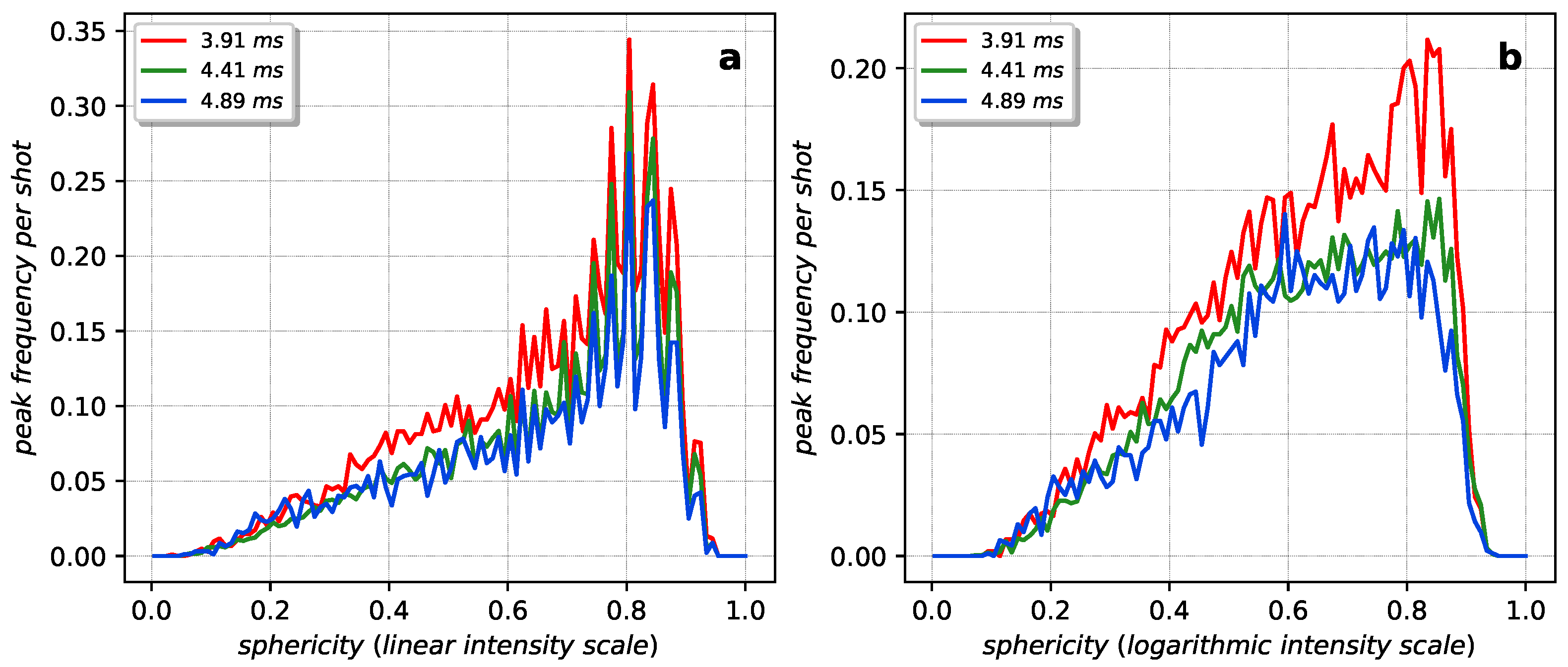
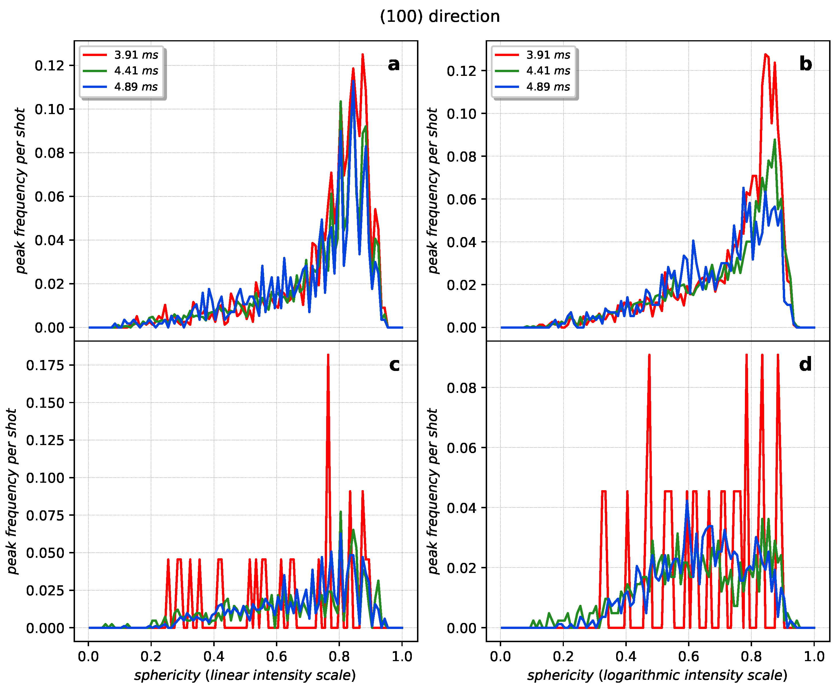
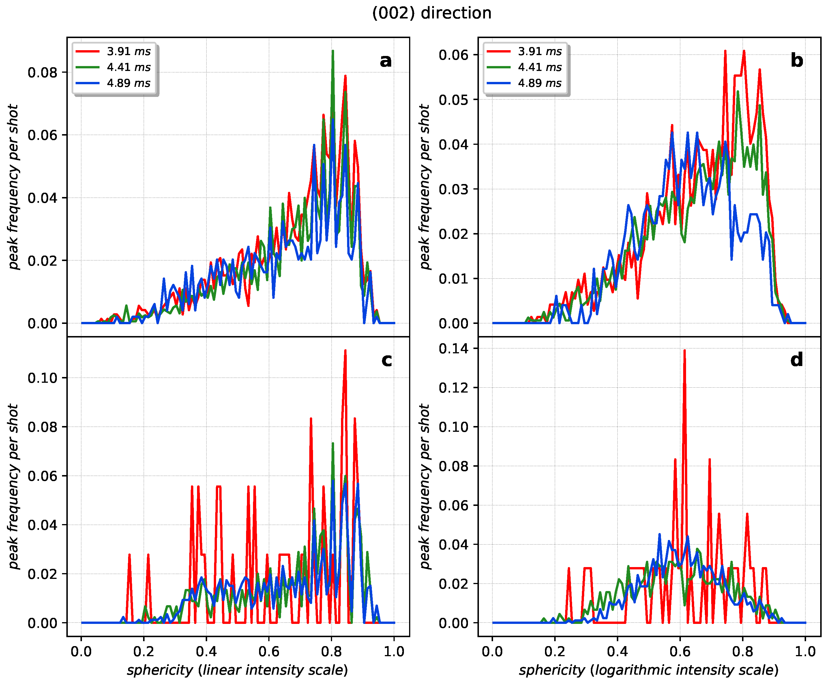
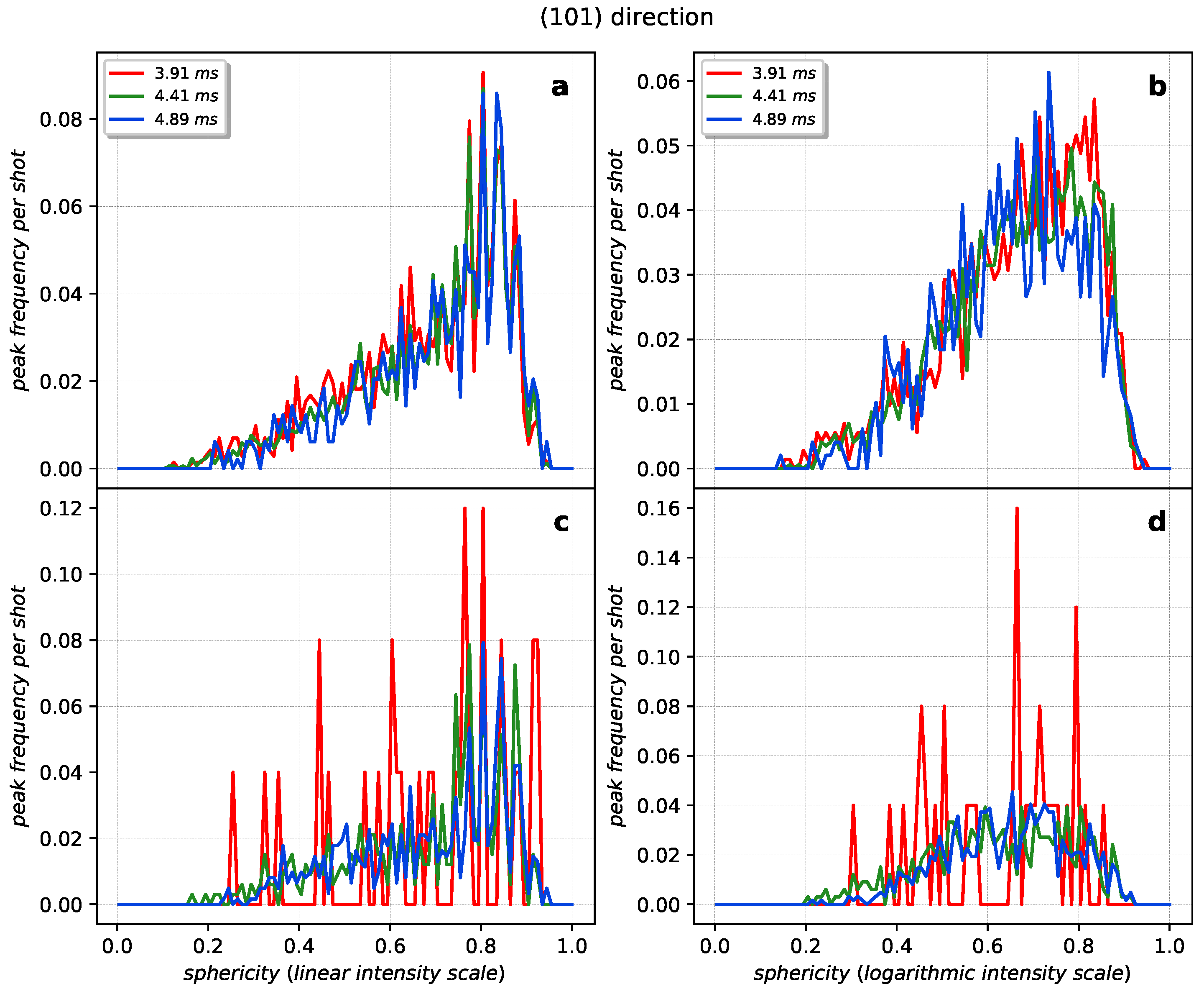
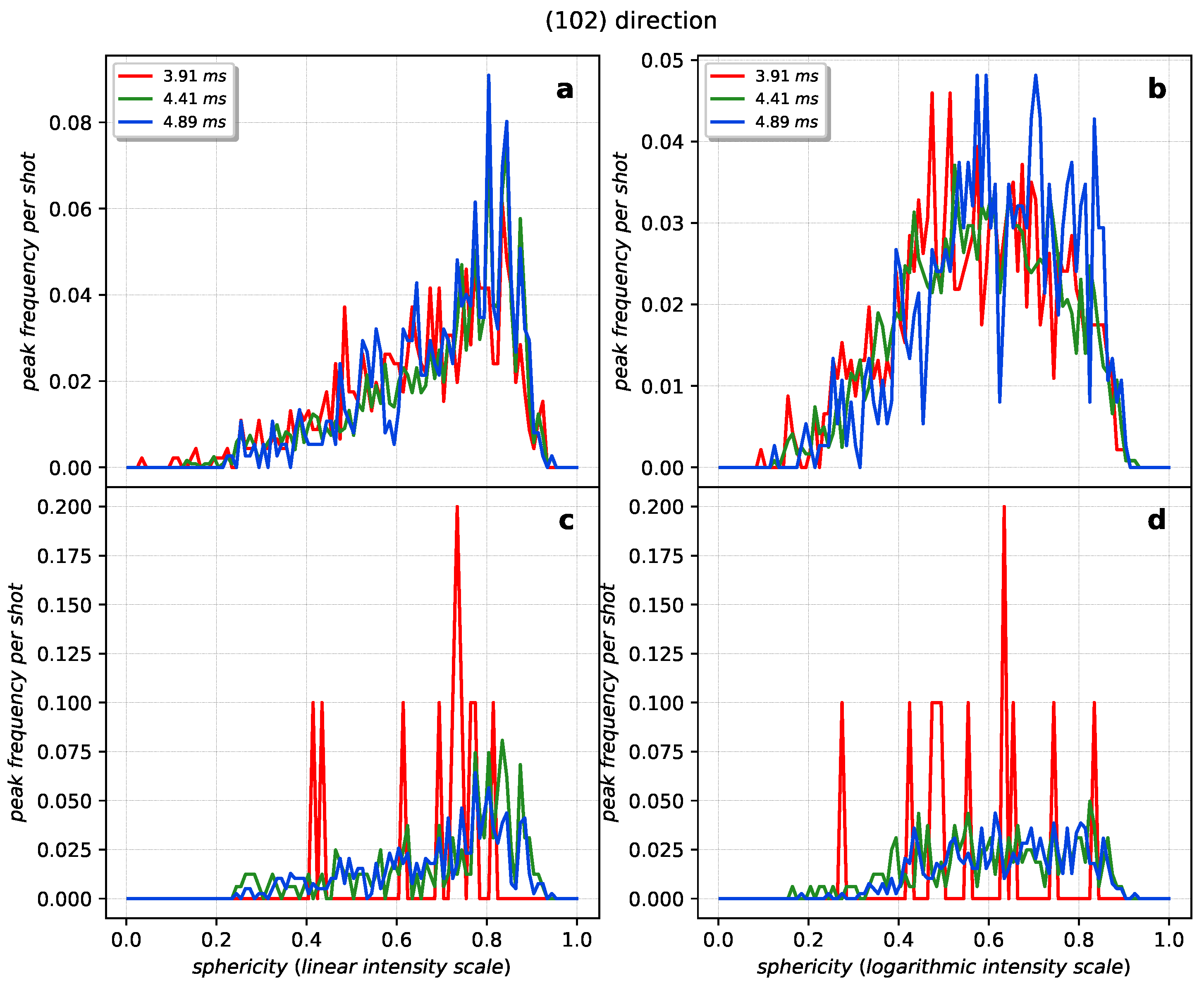
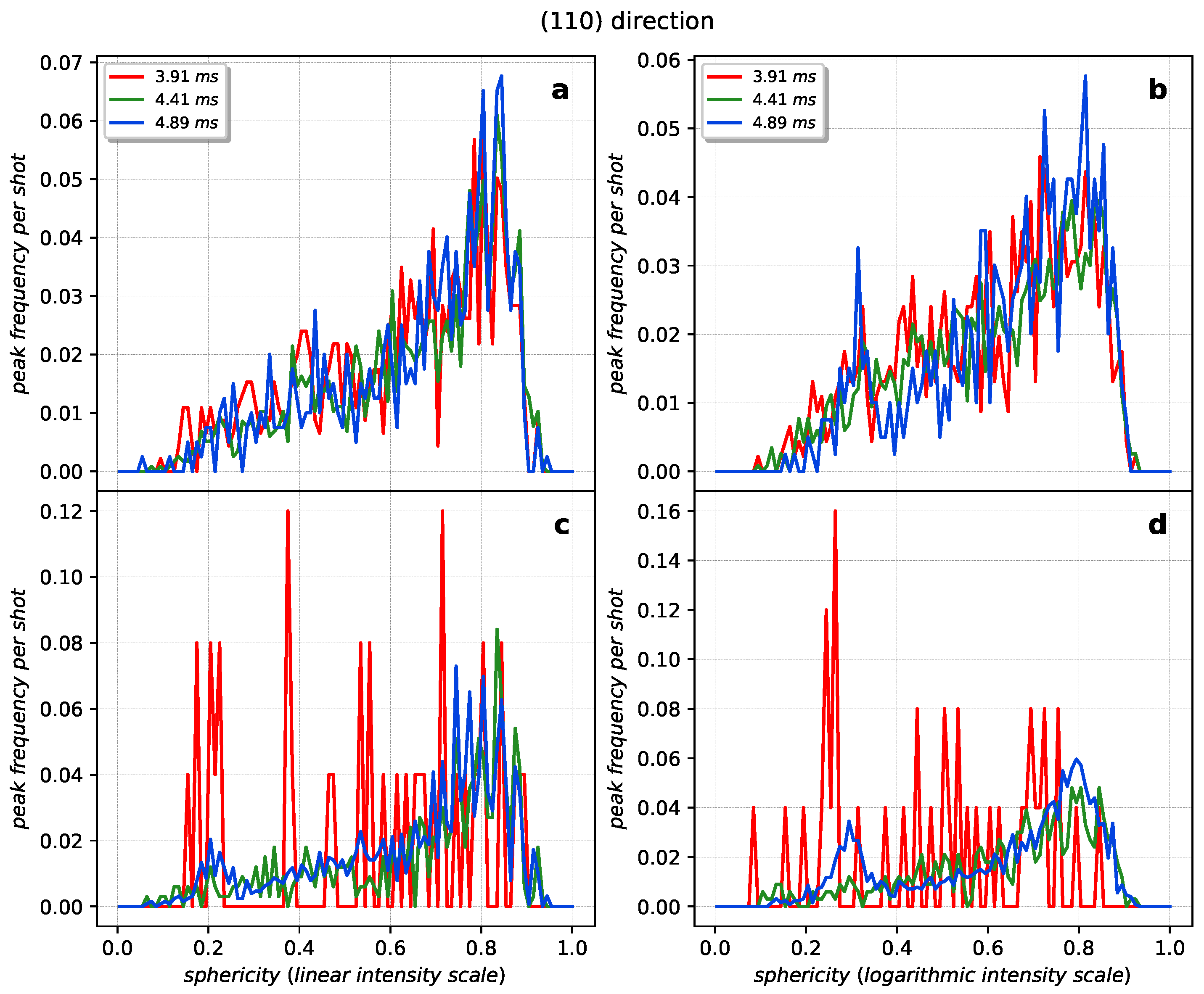
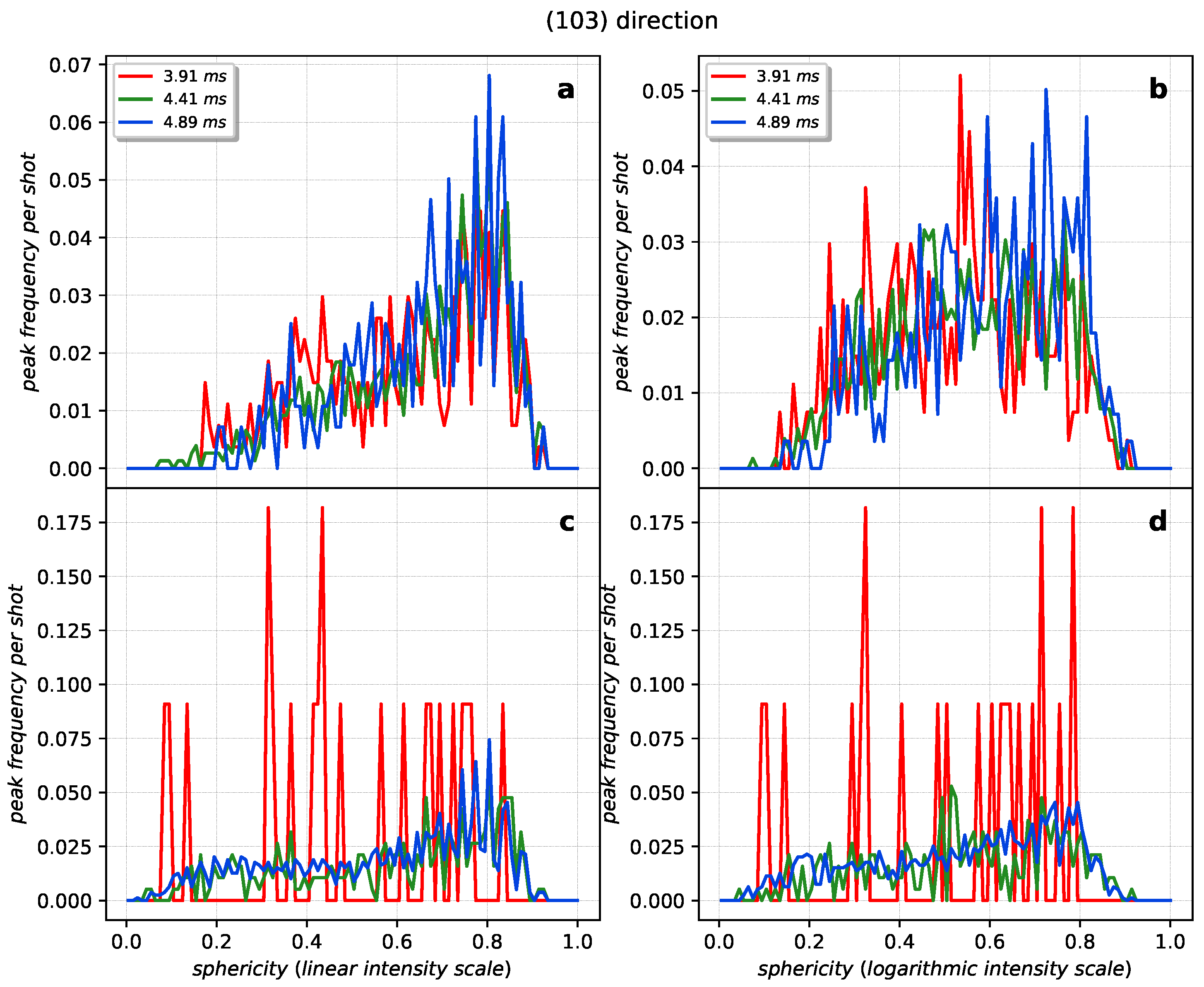
Appendix A.1. Sphericity and Relative Intensity Statistics


Appendix A.2. Gaussian Filtering and Contour Detection

Appendix A.3. Cubicity Estimate


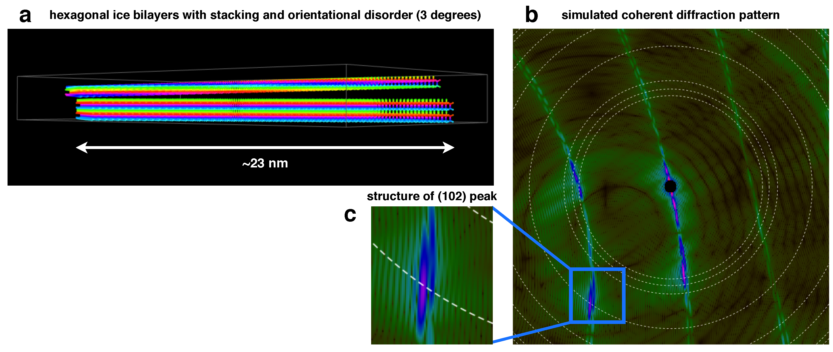
Appendix A.4. Stacking and Orientational Disorder Observed in Single-Shot Diffraction Patterns


References
- Day, J.A.; Schaefer, V.J. Peterson First Guides, Clouds and Weather; Houghton Mifflin: New York, NY, USA, 1991; p. 128. [Google Scholar]
- Fan, J.; Meng, J.; Ludescher, J.; Chen, X.; Ashkenazy, Y.; Kurths, J.; Havlin, S.; Schellnhuber, H.J. Statistical physics approaches to the complex Earth system. Phys. Rep. 2021, 896, 1–84. [Google Scholar] [CrossRef]
- Fossum, K.N.; Ovadnevaite, J.; Ceburnis, D.; Preißler, J.; Snider, J.R.; Huang, R.J.; Zuend, A.; O’Dowd, C. Sea-spray regulates sulfate cloud droplet activation over oceans. NPJ Clim. Atmos. Sci. 2020, 3, 14. [Google Scholar] [CrossRef] [Green Version]
- Kaufman, Y.J.; Tanré, D.; Boucher, O. A satellite view of aerosols in the climate system. Nature 2002, 419, 215–223. [Google Scholar] [CrossRef]
- Seinfeld, J.H.; Bretherton, C.; Carslaw, K.S.; Coe, H.; DeMott, P.J.; Dunlea, E.J.; Feingold, G.; Ghan, S.; Guenther, A.B.; Kahn, R.; et al. Improving our fundamental understanding of the role of aerosol-cloud interactions in the climate system. Proc. Natl. Acad. Sci. USA 2016, 113, 5781–5790. [Google Scholar] [CrossRef] [PubMed] [Green Version]
- Murray, B.J.; O’Sullivan, D.; Atkinson, J.D.; Webb, M.E. Ice nucleation by particles immersed in supercooled cloud droplets. Chem. Soc. Rev. 2012, 41, 6519–6554. [Google Scholar] [CrossRef] [PubMed] [Green Version]
- Hoose, C.; Möhler, O. Heterogeneous ice nucleation on atmospheric aerosols: A review of results from laboratory experiments. Atmos. Chem. Phys. 2012, 12, 9817–9854. [Google Scholar] [CrossRef] [Green Version]
- Fletcher, N.H. Size effect in heterogeneous nucleation. J. Chem. Phys. 1958, 29, 572–576. [Google Scholar] [CrossRef]
- Li, T.; Donadio, D.; Russo, G.; Galli, G. Homogeneous ice nucleation from supercooled water. Phys. Chem. Chem. Phys. 2011, 13, 19807–19813. [Google Scholar] [CrossRef]
- Reinhardt, A.; Doye, J.P. Free energy landscapes for homogeneous nucleation of ice for a monatomic water model. J. Chem. Phys. 2012, 136, 1–11. [Google Scholar] [CrossRef] [Green Version]
- Takahashi, T.; Kobayashi, T. The role of the cubic structure in freezing of a supercooled water droplet on an ice substrate. J. Cryst. Growth 1983, 64, 593–603. [Google Scholar] [CrossRef]
- Kobayashi, T.; Furukawa, Y.; Takahashi, T.; Uyeda, H. Cubic structure models at the junctions in polycrystalline snow crystals. J. Cryst. Growth 1976, 35, 262–268. [Google Scholar] [CrossRef]
- Ghaani, M.R.; Bernardi, M.; English, N.J. Crystallisation competition between cubic and hexagonal ice structures: Molecular-dynamics insight. Mol. Simul. 2021, 47, 18–26. [Google Scholar] [CrossRef]
- Hudait, A.; Qiu, S.; Lupi, L.; Molinero, V. Free energy contributions and structural characterization of stacking disordered ices. Phys. Chem. Chem. Phys. 2016, 18, 9544–9553. [Google Scholar] [CrossRef] [PubMed]
- Amaya, A.J.; Pathak, H.; Modak, V.P.; Laksmono, H.; Loh, N.D.; Sellberg, J.A.; Sierra, R.G.; McQueen, T.A.; Hayes, M.J.; Williams, G.J.; et al. How Cubic Can Ice Be? J. Phys. Chem. Lett. 2017, 8, 3216–3222. [Google Scholar] [CrossRef] [PubMed] [Green Version]
- Moore, E.B.; Molinero, V. Is it cubic? Ice crystallization from deeply supercooled water. Phys. Chem. Chem. Phys. 2011, 13, 20008–20016. [Google Scholar] [CrossRef]
- Johnston, J.C.; Molinero, V. Crystallization, melting, and structure of water nanoparticles at atmospherically relevant temperatures. J. Am. Chem. Soc. 2012, 134, 6650–6659. [Google Scholar] [CrossRef]
- Mason, B.J. The supercooling and nucleation of water. Adv. Phys. 1958, 7, 221–234. [Google Scholar] [CrossRef]
- Li, T.; Donadio, D.; Galli, G. Ice nucleation at the nanoscale probes no man’s land of water. Nat. Commun. 2013, 4, 1887. [Google Scholar] [CrossRef]
- Huang, J.; Bartell, L.S. Kinetics of Homogeneous Nucleation in the Freezing of Large Water Clusters. J. Phys. Chem. 1995, 99, 3924–3931. [Google Scholar] [CrossRef]
- Malkin, T.L.; Murray, B.J.; Brukhno, A.V.; Anwar, J.; Salzmann, C.G. Structure of ice crystallized from supercooled water. Proc. Natl. Acad. Sci. USA 2012, 109, 1041–1045. [Google Scholar] [CrossRef] [Green Version]
- Murray, B.J.; Knopf, D.A.; Bertram, A.K. The formation of cubic ice under conditions relevant to Earth’s atmosphere. Nature 2005, 434, 202–205. [Google Scholar] [CrossRef] [PubMed]
- Murray, B.J.; Bertram, A.K. Formation and stability of cubic ice in water droplets. Phys. Chem. Chem. Phys. 2006, 8, 186–192. [Google Scholar] [CrossRef] [PubMed] [Green Version]
- Guan, S.H.; Shang, C.; Huang, S.D.; Liu, Z.P. Two-Stage Solid-Phase Transition of Cubic Ice to Hexagonal Ice: Structural Origin and Kinetics. J. Phys. Chem. C 2018, 122, 29009–29016. [Google Scholar] [CrossRef]
- Fletcher, N.H. Structural diffusion, interface structure and crystal growth. J. Cryst. Growth 1975, 28, 375–384. [Google Scholar] [CrossRef]
- Thürmer, K.; Nie, S. Formation of hexagonal and cubic ice during low-temperature growth. Proc. Natl. Acad. Sci. USA 2013, 110, 11757–11762. [Google Scholar] [CrossRef] [PubMed] [Green Version]
- Hansen, T.C.; Koza, M.M.; Kuhs, W.F. Formation and annealing of cubic ice: I. Modelling of stacking faults. J. Phys. Condens. Matter 2008, 20, 285104. [Google Scholar] [CrossRef]
- Hansen, T.C.; Koza, M.M.; Lindner, P.; Kuhs, W.F. Formation and annealing of cubic ice: II. Kinetic study. J. Phys. Condens. Matter 2008, 20, 285105. [Google Scholar] [CrossRef]
- Kuhs, W.F.; Sippel, C.; Falenty, A.; Hansen, T.C. Extent and relevance of stacking disorder in “ice Ic”. Proc. Natl. Acad. Sci. USA 2012, 109, 21259–21264. [Google Scholar] [CrossRef] [PubMed] [Green Version]
- Malkin, T.L.; Murray, B.J.; Salzmann, C.G.; Molinero, V.; Pickering, S.J.; Whale, T.F. Stacking disorder in ice I. Phys. Chem. Chem. Phys. 2015, 17, 60–76. [Google Scholar] [CrossRef] [Green Version]
- Haji-Akbari, A. Ice and its formation. In Antifreeze Proteins Volume 1: Environment, Systematics and Evolution; Ramløv, H., Friis, D.S., Eds.; Springer International Publishing: Cham, Switzerland, 2020; pp. 13–51. [Google Scholar] [CrossRef]
- Tarn, M.D.; Sikora, S.N.; Porter, G.C.; Shim, J.U.; Murray, B.J. Homogeneous freezing of water using microfluidics. Micromachines 2021, 12, 223. [Google Scholar] [CrossRef]
- Lupi, L.; Hudait, A.; Peters, B.; Grünwald, M.; Gotchy Mullen, R.; Nguyen, A.H.; Molinero, V. Role of stacking disorder in ice nucleation. Nature 2017, 551, 218–222. [Google Scholar] [CrossRef] [PubMed]
- Del Rosso, L.; Celli, M.; Grazzi, F.; Catti, M.; Hansen, T.C.; Fortes, A.D.; Ulivi, L. Cubic ice Ic without stacking defects obtained from ice XVII. Nat. Mater. 2020, 19, 663–668. [Google Scholar] [CrossRef]
- Komatsu, K.; Machida, S.; Noritake, F.; Hattori, T.; Sano-Furukawa, A.; Yamane, R.; Yamashita, K.; Kagi, H. Ice Ic without stacking disorder by evacuating hydrogen from hydrogen hydrate. Nat. Commun. 2020, 11, 2–4. [Google Scholar] [CrossRef] [Green Version]
- Libbrecht, K.G. The physics of snow crystals. Rep. Prog. Phys. 2005, 68, 855–895. [Google Scholar] [CrossRef] [Green Version]
- Mossop, S.C. Concentrations of ice crystals in clouds. Bull. Am. Meteorol. Soc. 1970, 51, 474–479. [Google Scholar] [CrossRef] [Green Version]
- King, B.F.; Weinhold, F. Structure and spectroscopy of (HCN)n clusters: Cooperative and electronic delocalization effects in C–H-N hydrogen bonding. J. Chem. Phys. 1995, 103, 333. [Google Scholar] [CrossRef]
- Hashino, T.; De Boer, G.; Okamoto, H.; Tripoli, G.J. Relationships between immersion freezing and crystal habit for arctic mixed-phase clouds-A numerical study. J. Atmos. Sci. 2020, 77, 2411–2438. [Google Scholar] [CrossRef]
- Leisner, T.; Duft, D.; Möhler, O.; Saathoff, H.; Schnaiter, M.; Henin, S.; Stelmaszczyk, K.; Petrarca, M.; Delagrange, R.; Hao, Z.; et al. Laser-induced plasma cloud interaction and ice multiplication under cirrus cloud conditions. Proc. Natl. Acad. Sci. USA 2013, 110, 10106–10110. [Google Scholar] [CrossRef] [Green Version]
- Zhao, B.; Liou, K.N.; Gu, Y.; Jiang, J.H.; Li, Q.; Fu, R.; Huang, L.; Liu, X.; Shi, X.; Su, H.; et al. Impact of aerosols on ice crystal size. Atmos. Chem. Phys. 2018, 18, 1065–1078. [Google Scholar] [CrossRef] [Green Version]
- Espinosa, J.R.; Vega, C.; Sanz, E. Homogeneous Ice Nucleation Rate in Water Droplets. J. Phys. Chem. C 2018, 122, 22892–22896. [Google Scholar] [CrossRef] [Green Version]
- King, W.D.; Fletcher, N.H. Pressures and stresses in freezing water drops. J. Phys. D Appl. Phys. 1973, 6, 2157–2173. [Google Scholar] [CrossRef] [Green Version]
- Wildeman, S.; Sterl, S.; Sun, C.; Lohse, D. Fast Dynamics of Water Droplets Freezing from the Outside in. Phys. Rev. Lett. 2017, 118, 1–5. [Google Scholar] [CrossRef] [Green Version]
- DePonte, D.P.; Weierstall, U.; Schmidt, K.; Warner, J.; Starodub, D.; Spence, J.C.H.; Doak, R.B. Gas Dynamic Virtual Nozzle for Generation of Microscopic Droplet Streams. J. Phys. D Appl. Phys. 2008, 41, 195505. [Google Scholar] [CrossRef] [Green Version]
- Laksmono, H.; McQueen, T.A.; Sellberg, J.A.; Loh, N.D.; Huang, C.; Schlesinger, D.; Sierra, R.G.; Hampton, C.Y.; Nordlund, D.; Beye, M.; et al. Anomalous behavior of the homogeneous ice nucleation rate in “no-man’s land”. J. Phys. Chem. Lett. 2015, 6, 2826–2832. [Google Scholar] [CrossRef] [PubMed] [Green Version]
- Sellberg, J.A.; Huang, C.; McQueen, T.A.; Loh, N.D.; Laksmono, H.; Schlesinger, D.; Sierra, R.G.; Nordlund, D.; Hampton, C.Y.; Starodub, D.; et al. Ultrafast X-ray probing of water structure below the homogeneous ice nucleation temperature. Nature 2014, 510, 381–384. [Google Scholar] [CrossRef] [PubMed]
- Schlesinger, D.; Sellberg, J.A.; Nilsson, A.; Pettersson, L.G. Evaporative cooling of microscopic water droplets in vacuo: Molecular dynamics simulations and kinetic gas theory. J. Chem. Phys. 2016, 144, 124502. [Google Scholar] [CrossRef] [Green Version]
- Pathak, H.; Späh, A.; Esmaeildoost, N.; Sellberg, J.A.; Kim, K.H.; Perakis, F.; Amann-Winkel, K.; Ladd-Parada, M.; Koliyadu, J.; Lane, T.J.; et al. Enhancement and maximum in the isobaric specific-heat capacity measurements of deeply supercooled water using ultrafast calorimetry. Proc. Natl. Acad. Sci. USA 2021, 118, e2018379118. [Google Scholar] [CrossRef]
- Hart, P.; Boutet, S.; Carini, G.; Dragone, A.; Duda, B.; Freytag, D.; Haller, G.; Herbst, R.; Herrmann, S.; Kenney, C.; et al. The comell-SLAC pixel array detector at LCLS. In Proceedings of the 2012 IEEE Nuclear Science Symposium and Medical Imaging Conference, Anaheim, CA, USA, 27 October–3 November 2012; pp. 538–541. [Google Scholar]
- Dowell, L.G.; Rinfret, A.P. Low-Temperature Forms of Ice as Studied by X-ray Diffraction. Nature 1960, 188, 1144–1148. [Google Scholar] [CrossRef]
- Casas-Cabanas, M.; Reynaud, M.; Rikarte, J.; Horbach, P.; Rodriguez-Carvajal, J. FAULTS: A program for refinement of structures with extended defects. J. Appl. Crystallogr. 2016, 49, 2259–2269. [Google Scholar] [CrossRef]
- Barty, A.; Kirian, R.A.; Maia, F.R.; Hantke, M.; Yoon, C.H.; White, T.A.; Chapman, H. Cheetah: Software for high-throughput reduction and analysis of serial femtosecond X-ray diffraction data. J. Appl. Crystallogr. 2014, 47, 1118–1131. [Google Scholar] [CrossRef] [Green Version]
- Hadian-Jazi, M.; Messerschmidt, M.; Darmanin, C.; Giewekemeyer, K.; Mancuso, A.P.; Abbey, B. A peak-finding algorithm based on robust statistical analysis in serial crystallography. J. Appl. Crystallogr. 2017, 50, 1705–1715. [Google Scholar] [CrossRef]
- Peters, J. The ‘seed-skewness’ integration method generalized for three-dimensional Bragg peaks. J. Appl. Crystallogr. 2003, 36, 1475–1479. [Google Scholar] [CrossRef]
- Wilkinson, C.; Khamis, H.W.; Stansfield, R.F.; McIntyre, G.J. Integration of single-crystal reflections using area multidetectors. J. Appl. Crystallogr. 1988, 21, 471–478. [Google Scholar] [CrossRef]
- Sonka, M.; Hlavac, V.; Boyle, R. Segmentation. In Image Processing, Analysis and Machine Vision; Springer: Boston, MA, USA, 1993; pp. 112–191. [Google Scholar] [CrossRef]
- Yan, F.; Zhang, H.; Kube, C.R. A multistage adaptive thresholding method. Pattern Recognit. Lett. 2005, 26, 1183–1191. [Google Scholar] [CrossRef]
- Otsu, N. A Threshold Selection Method from Gray-Level Histograms. IEEE Trans. Syst. Man Cybern. 1979, 9, 62–66. [Google Scholar] [CrossRef] [Green Version]
- Rogowska, J. Overview and Fundamentals of Medical Image Segmentation, 2nd ed.; Elsevier Inc.: Amsterdam, The Netherlands, 2009; pp. 73–90. [Google Scholar] [CrossRef]
- Wadell, H. Volume, Shape, and Roundness of Rock Particles. J. Geol. 1932, 40, 443–451. [Google Scholar] [CrossRef]
- La Placa, S.J.; Post, B. Thermal expansion of ice. Acta Crystallogr. 1960, 13, 503–505. [Google Scholar] [CrossRef]
- Amaya, A.J.; Wyslouzil, B.E. Ice nucleation rates near 225 K. J. Chem. Phys. 2018, 148. [Google Scholar] [CrossRef] [PubMed]
- Kohl, I.; Mayer, E.; Hallbrucker, A. The glassy water–cubic ice system: A comparative study by X-ray diffraction and differential scanning calorimetry. Phys. Chem. Chem. Phys. 2000, 2, 1579–1586. [Google Scholar] [CrossRef]
- Jung, S.; Tiwari, M.K.; Doan, N.V.; Poulikakos, D. Mechanism of supercooled droplet freezing on surfaces. Nat. Commun. 2012, 3, 1–8. [Google Scholar] [CrossRef] [Green Version]
- Riechers, B.; Wittbracht, F.; Hütten, A.; Koop, T. The homogeneous ice nucleation rate of water droplets produced in a microfluidic device and the role of temperature uncertainty. Phys. Chem. Chem. Phys. 2013, 15, 5873–5887. [Google Scholar] [CrossRef]
- Xue, H.; Fu, Y.; Lu, Y.; Hao, D.; Li, K.; Bai, G.; Ou-Yang, Z.C.; Wang, J.; Zhou, X. Spontaneous Freezing of Water between 233 and 235 K Is Not Due to Homogeneous Nucleation. J. Am. Chem. Soc. 2021, 143, 13548–13556. [Google Scholar] [CrossRef] [PubMed]
- Stan, C.A.; Schneider, G.F.; Shevkoplyas, S.S.; Hashimoto, M.; Ibanescu, M.; Wiley, B.J.; Whitesides, G.M. A microfluidic apparatus for the study of ice nucleation in supercooled water drops. Lab A Chip 2009, 9, 2293–2305. [Google Scholar] [CrossRef] [PubMed]
- Schremb, M.; Tropea, C. Solidification of supercooled water in the vicinity of a solid wall. Phys. Rev. E 2016, 94, 52804. [Google Scholar] [CrossRef]
- Altarelli, M.; Kurta, R.P.; Vartanyants, I.A. X-ray cross-correlation analysis and local symmetries of disordered systems: General theory. Phys. Rev. B 2010, 82, 104207. [Google Scholar] [CrossRef] [Green Version]
- Mendez, D.; Lane, T.; Sung, J.; Sellberg, J.; Levard, C.; Watkins, H.; Cohen, A.; Soltis, M.; Sutton, S.; Spudich, J.; et al. Observation of correlated X-ray scattering at atomic resolution. Philos. Trans. R. Soc. B Biol. Sci. 2014, 369. [Google Scholar] [CrossRef] [PubMed] [Green Version]
- Mendez, D.; Watkins, H.; Qiao, S.; Raines, K.S.; Lane, T.J.; Schenk, G.; Nelson, G.; Subramanian, G.; Tono, K.; Joti, Y.; et al. Angular correlations of photons from solution diffraction at a free-electron laser encode molecular structure. IUCrJ 2016, 3, 420–429. [Google Scholar] [CrossRef]


| Travel Time (ms) | T (K) | Total Hits | Total Peaks | Hits above 50 ADU/pixel | Hits below 50 ADU/pixel | Peaks above 50 ADU/pixel | Peaks below 50 ADU/pixel |
|---|---|---|---|---|---|---|---|
| 3.91 | 230 | 1113 | 8997 | 1034 | 79 | 8708 | 289 |
| 4.41 | 229 | 3985 | 21,575 | 2771 | 1214 | 18,005 | 3570 |
| 4.89 | 228 | 3457 | 25,936 | 920 | 2537 | 5402 | 20,534 |
| Directions (hkl) | Travel Time (ms) | Hits ≥ 50 ADU/pixel | Hits < 50 ADU/pixel | Peaks ≥ 50 ADU/pixel | Peaks < 50 ADU/pixel | Circular Peaks ADU/pixel | Non-Circular Peaks ADU/pixel | Structured Peaks ADU/pixel | Circular Peaks ADU/pixel | Non-Circular Peaks ADU/pixel | Structured Peaks ADU/pixel |
|---|---|---|---|---|---|---|---|---|---|---|---|
| (100) | 3.91 | 776 | 22 | 1547 | 26 | 1039 | 25 | 251 | 9 | 2 | 6 |
| 4.41 | 1846 | 414 | 3030 | 456 | 1867 | 80 | 505 | 179 | 17 | 43 | |
| 4.89 | 567 | 828 | 913 | 949 | 500 | 21 | 165 | 425 | 16 | 151 | |
| (002) | 3.91 | 723 | 36 | 1314 | 45 | 473 | 39 | 520 | 16 | 0 | 9 |
| 4.41 | 1602 | 451 | 2526 | 504 | 874 | 55 | 939 | 135 | 7 | 121 | |
| 4.89 | 493 | 864 | 707 | 958 | 189 | 23 | 284 | 327 | 12 | 268 | |
| (101) | 3.91 | 717 | 25 | 1267 | 33 | 473 | 30 | 405 | 14 | 0 | 7 |
| 4.41 | 1714 | 331 | 2850 | 412 | 1206 | 59 | 810 | 146 | 10 | 91 | |
| 4.89 | 489 | 618 | 790 | 733 | 326 | 14 | 259 | 287 | 8 | 168 | |
| (102) | 3.91 | 457 | 10 | 666 | 11 | 178 | 31 | 313 | 4 | 0 | 4 |
| 4.41 | 1213 | 161 | 1712 | 199 | 636 | 54 | 675 | 76 | 9 | 66 | |
| 4.89 | 374 | 389 | 569 | 442 | 223 | 12 | 200 | 181 | 6 | 121 | |
| (110) | 3.91 | 458 | 25 | 695 | 39 | 168 | 22 | 387 | 6 | 1 | 26 |
| 4.41 | 1165 | 333 | 1668 | 429 | 503 | 54 | 829 | 137 | 7 | 114 | |
| 4.89 | 399 | 1275 | 593 | 1897 | 210 | 25 | 240 | 755 | 103 | 669 | |
| (103) | 3.91 | 269 | 11 | 345 | 22 | 69 | 15 | 209 | 3 | 0 | 16 |
| 4.41 | 760 | 189 | 979 | 266 | 259 | 47 | 507 | 57 | 8 | 143 | |
| 4.89 | 279 | 793 | 383 | 1295 | 104 | 11 | 179 | 290 | 19 | 709 | |
| (200), (112), (201) | 3.91 | 408 | 13 | 537 | 34 | 206 | 6 | 183 | 1 | 1 | 29 |
| 4.41 | 873 | 209 | 1111 | 533 | 429 | 21 | 368 | 57 | 4 | 3718 | |
| 4.89 | 254 | 967 | 332 | 6305 | 115 | 7 | 105 | 110 | 40 | 6028 |
Publisher’s Note: MDPI stays neutral with regard to jurisdictional claims in published maps and institutional affiliations. |
© 2022 by the authors. Licensee MDPI, Basel, Switzerland. This article is an open access article distributed under the terms and conditions of the Creative Commons Attribution (CC BY) license (https://creativecommons.org/licenses/by/4.0/).
Share and Cite
Esmaeildoost, N.; Jönsson, O.; McQueen, T.A.; Ladd-Parada, M.; Laksmono, H.; Loh, N.-T.D.; Sellberg, J.A. Heterogeneous Ice Growth in Micron-Sized Water Droplets Due to Spontaneous Freezing. Crystals 2022, 12, 65. https://0-doi-org.brum.beds.ac.uk/10.3390/cryst12010065
Esmaeildoost N, Jönsson O, McQueen TA, Ladd-Parada M, Laksmono H, Loh N-TD, Sellberg JA. Heterogeneous Ice Growth in Micron-Sized Water Droplets Due to Spontaneous Freezing. Crystals. 2022; 12(1):65. https://0-doi-org.brum.beds.ac.uk/10.3390/cryst12010065
Chicago/Turabian StyleEsmaeildoost, Niloofar, Olof Jönsson, Trevor A. McQueen, Marjorie Ladd-Parada, Hartawan Laksmono, Ne-Te Duane Loh, and Jonas A. Sellberg. 2022. "Heterogeneous Ice Growth in Micron-Sized Water Droplets Due to Spontaneous Freezing" Crystals 12, no. 1: 65. https://0-doi-org.brum.beds.ac.uk/10.3390/cryst12010065