
A New Exponential Distribution to Model Concrete Compressive Strength Data


1
Department of Mathematical Sciences, College of Science, Princess Nourah bint Abdulrahman University, Riyadh 11671, Saudi Arabia
2
Department of Statistics, Faculty of Science, King Abdulaziz University, Jeddah 21589, Saudi Arabia
3
Department of Statistics, Faculty of Commerce, Zagazig University, Zagazig 44519, Egypt
*
Author to whom correspondence should be addressed.
Crystals 2022, 12(3), 431; https://0-doi-org.brum.beds.ac.uk/10.3390/cryst12030431
Submission received: 25 February 2022
/
Revised: 17 March 2022
/
Accepted: 17 March 2022
/
Published: 20 March 2022
Abstract
:Concrete mixtures can be developed to deliver a broad spectrum of mechanical and durability properties to satisfy the configuration conditions of construction. One technique for evaluating the compressive strength of concrete is to suppose that it pursues a probabilistic model from which it is reliability estimated. In this paper, a new technique to generate probability distributions is considered and a new three-parameter exponential distribution as a new member of the new family is presented in detail. The proposed distribution is able to model the compressive strength of high-performance concrete rather than some other competitive models. The new distribution delivers decreasing, increasing, upside-down bathtub and bathtub-shaped hazard rates. The maximum likelihood estimation approach is used to estimate model parameters as well as the reliability function. The approximate confidence intervals of these quantities are also obtained. To assess the performance of the point and interval estimations, a simulation study was conducted. We demonstrate the performance of the offered new distribution by investigating one high-performance concrete compressive strength dataset. The numerical outcomes showed that the maximum likelihood method provides consistent and asymptotically unbiased estimators. The estimates of the unknown parameters as well as the reliability function perform well as sample size increases in terms of minimum mean square error. The confidence interval of the reliability function has an appropriate length utilizing the delta method. Moreover, the real data analysis indicated that the new distribution is more suitable when compared to some well-known and some recently proposed distributions to evaluate the reliability of concrete mixtures.
1. Introduction
In fact, concrete is a widely used construction material in the world. Concrete compressive strength is a criterion employed in specifying the portion of resistance a structural component can deliver to deformation. Compressive strength is a widely used standard to access the performance of a provided concrete mixture. This technique of assessing concrete is essential because it is the primary measure determining how sufficiently concrete can resist loads that impact its measure. It specifically informs us whether a distinct mixture is appropriate for encountering the conditions of a certain venture. Concrete can astoundingly stand up to compressive loading. This is a frequent reason for why it is useful for constructing arches, foundations, dams, columns and tunnel linings among other buildings.
Experimenters from various areas of science may endeavor to represent phenomena of interest, such as high-concrete concrete compressive strength, using probabilistic models. In recent years, many authors have exhibited significant appeal in representing new generalized families of probability distributions by adding one or more additional parameters to well-known distributions to yield new models with more incredible flexibility in modeling. The growth of proposing new statistical distributions is a major study area in the approach of distribution theory. Noteworthy methods include the following: the exponentiated method by Mudholkar and Srivastava [1], Marshall–Olkin method by Marshall and Olkin [2], beta-G family by Eugene et al.Olkin [3], Kumaraswamy-G family by Cordeiro and Castro [4], T-X family by Alzaatreh et al. [5], Weibull-G family by Bourguignon et al. [6], logarithmic transformed (LT) method by Pappas et al. [7], alpha power (AP) method by Mahdavi and Kundu [8], Marshall–Olkin AP method by Nassar et al. [9] and weighted AP transformed method by Alotaibi et al. [10]. For more details about other methods for generating distributions, one can refer to Lee et al. [11] and Jones [12].
Pappas et al. [7] proposed the LT approach, which uses a cumulative distribution function (CDF) and probability density function to induct a new parameter into well-known distributions (PDF), respectively.
Pappas et al. [7] considered the modified Weibull extension distribution by Xie et al. [13] as a baseline distribution G in (1) and studied some characteristics of the new distribution. Nassar et al. [14] used the LT method to propose a new form for the Weibull distribution. Eltehiwy [15] introduced the LT inverse Lindley distribution. Alotaibi et al. [16] utilized the CDF in (1) to introduce a new generalization for the traditional Lomax distribution.
Lately, Mahdavi and Kundu [8] offered the AP method for yielding new probability distributions by introducing an extra parameter to bring about a more elastic family. The CDF of the AP method is provided as follows:
and the corresponding PDF is the following.
Utilizing the AP method, a new AP Weibull (APW) distribution is proposed by Nassar et al. [17]. Dey et al. [18] introduced the AP inverse Lindley distribution. Ihtisham et al. [19] proposed the AP Pareto distribution. Eghwerido et al. [20,21] presented the AP Gompertz and AP Teissier distributions, respectively. Eghwerido et al. [22] proposed the AP-extended generalized exponential distribution.
The main goal of this article is to present a new method for generating probability distributions by using the AP CDF from (3) as the baseline CDF in (1). The logarithmic transformed alpha power (LTAP) family is the name given to the new family. The new LTAP family can be used to produce probability distributions with closed forms CDF and PDF. Firstly, we derive some structural properties of the LTAP family including the mixture representation for the PDF. Secondly, we assume the exponential as a baseline for the LTAP family and develop a new three-parameter LTAP-exponential (LTAPEx) distribution. The hazard rate functions (HRF) of the LTAPEx distribution accommodates monotonic, decreasing, increasing, upside-down bathtub and bathtub-shaped models. Therefore, the LTAPEx distribution can be used as a competitive model for many well-known distributions presented in the literature. Another motivation for the LTAPEx distribution is that it contains some sub-models such as exponential and alpha power exponential (APEx) distributions. Moreover, it can be considered as an appropriate model for modeling positively skewed data, which may not be suitably fitted by other standard distributions. The highly complex materials of high-performance concrete can render modeling its behavior an extremely difficult task. One of our practical objectives in this study is to evaluate the reliability of the high-performance concrete by assuming that the compressive strength of concrete follows the LTAPEx model. We then apply this model to a real high-performance concrete compressive strength dataset to check our findings. The outcomes of this analysis showed that the proposed model can be considered as an appropriate model when compared with some other competitive models to model high-performance concrete. The current study is an attempt to investigate and choose the most suitable model to assess the reliability of high-performance concrete, which we believe would be of outstanding appeal to reliability engineers.
The rest of the article is divided into the following sections: In Section 2, we present the LTAP family and provide a linear representation for the LTAP family PDF. In Section 3, we present the LTAPEx distribution. In Section 4, we study some properties of the LTAPEx distribution. The maximum likelihood method is considered to obtain the point and interval estimates for the model parameters as well as the corresponding reliability function (RF) in Section 5. A simulation study is conducted in Section 6. The investigation of one real dataset is provided in Section 7. Finally, Section 8 provides some conclusions.
2. The LTAP Family of Distributions
The CDF of the LTAP family is obtained by replacing in Equation (1) by of the APT class given by (3). We have the following.
Its PDF reduces to the following.
Henceforth, we denotea random variable having PDF in (6) by X. In the next subsections, some general properties of the LTAP family are derived.
2.1. Mixture Representation of the LTAP Family
Now, using the binomial expansion and the following two series:
the PDF of the LTAP family in (6) can be written, after some simplifications, in the following form:
where refers to the exponentiated-G (exp-G) PDF with shape parameter , and is given by the following.
The expansion in (8) provides the PDF of the LTAP family as a linear combination of the PDF of the exp-G family. Therefore, some structural properties of the new family can be obtained directly using this representation. In addition, the expansion of the CDF of the LTAP family can be derived by integrating (8), and it is stated as follows:
where is the CDF of the exp-G family with shape parameter .
2.2. Quantile Function of the LTAP Family
For the LTAP family, the quantile function can be reached by inverting (5) as follows.
Many beneficial measures can be calculated from (11), including the first quartile, median and third quartile by placing p with and , respectively. For example, the median of the LTAP family can be obtained as follows.
Different significant applications relative to the quantile function in (11) are used to simulate random samples from the LTAP family. Let , then one can generate a random sample consisting of n observations from the LTAP family as follows.
3. The LTAPEx Distribution
In this section, we explain the LTAPEx distribution and some associated statistical features. By entering , of the exponential distribution in (5), one can reach the CDF of the LTAPEx distribution as follows.
By differentiating (14) with respect to x, we can obtain the PDF of the LTAPEx distribution as follows:
where is the scale parameter, and and are the shape parameters. Moreover, the RF and the HRF of the LTAPEx distribution are furnished, respectively, by the following.
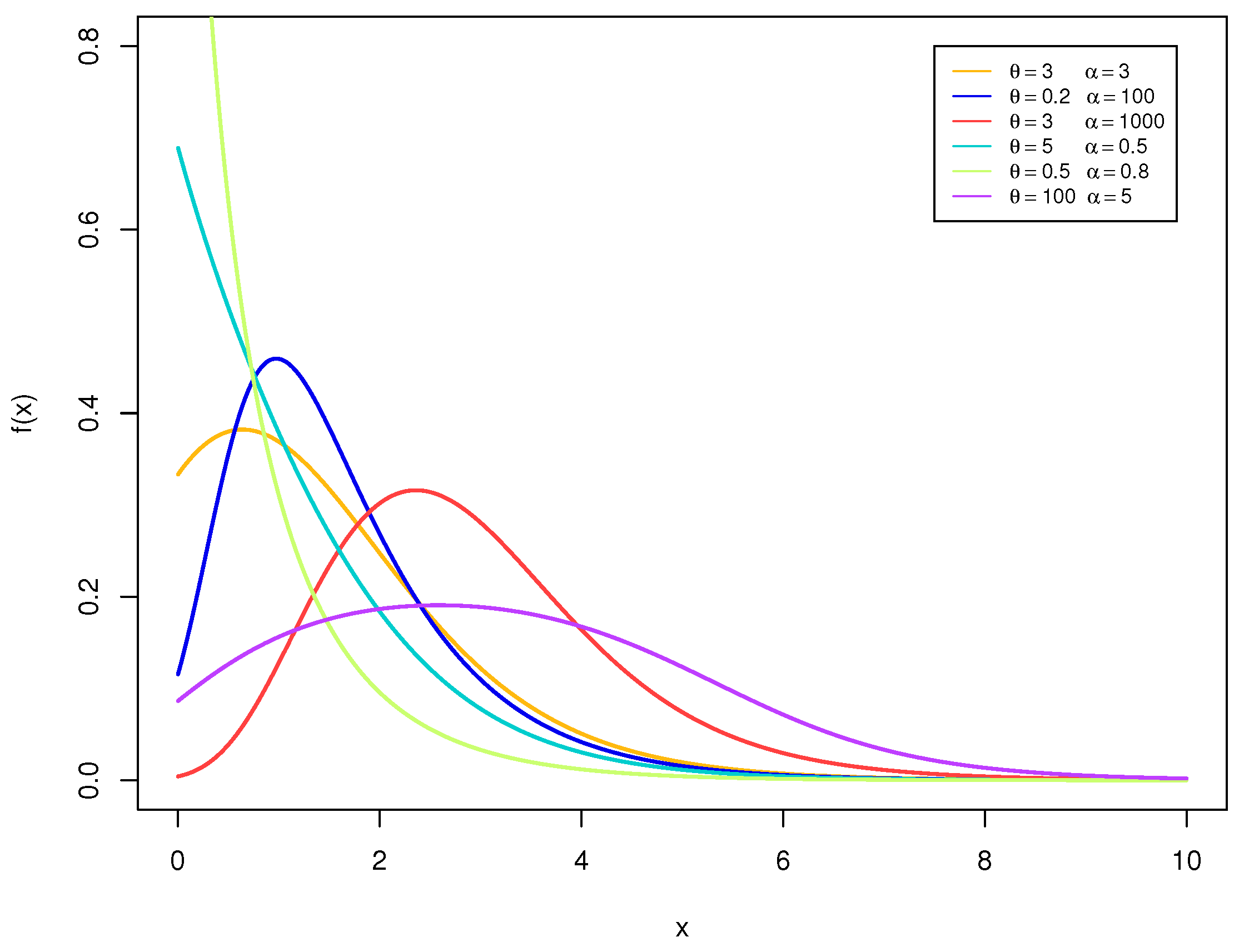
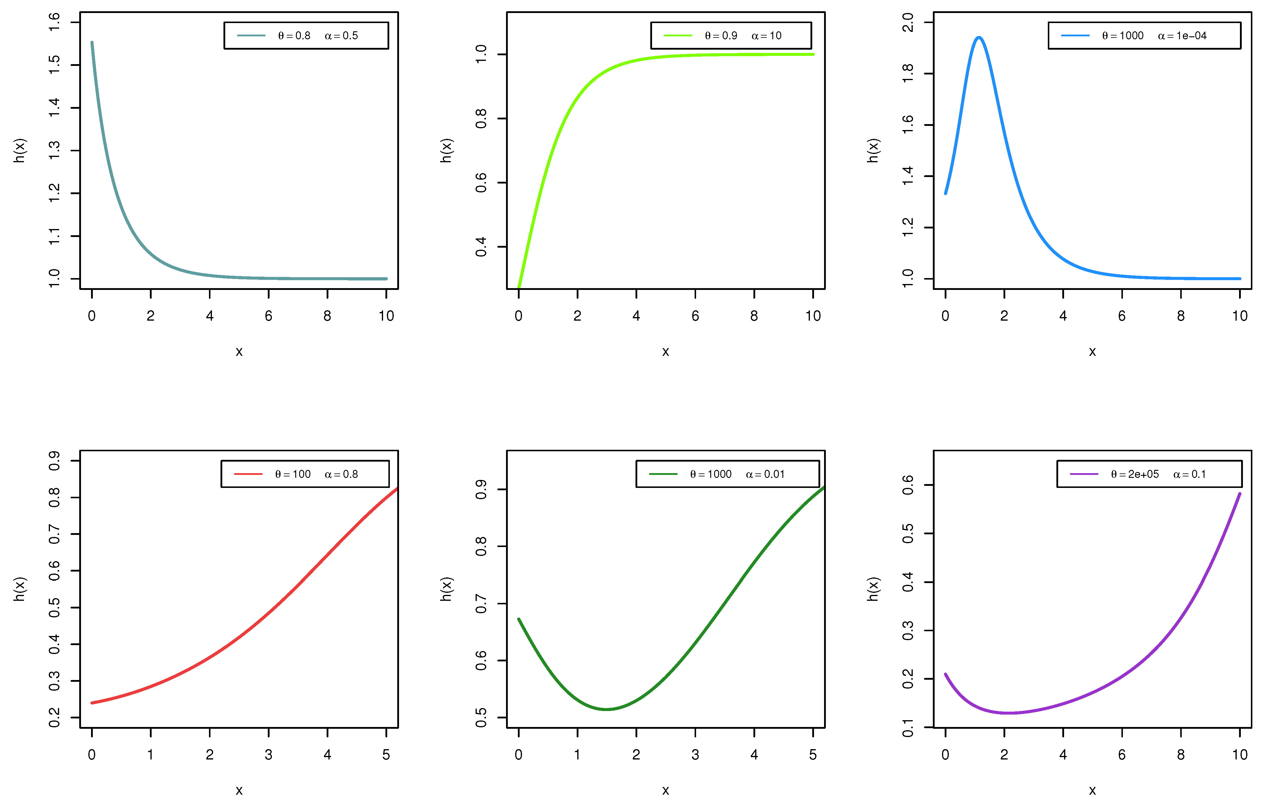
It can be observed here that when and tend to one, the PDF in (15) reduces to the PDF of the exponential distribution. Moreover, when , the LTAPEx distribution reduces to the alpha power exponential distribution proposed by Mahdavi and Kundu (2017). Another special case is when , the LTAPEx distribution reduces to the logarithmic transformed exponential distribution. Figure 1 layouts the various plots of the PDF of the LTAPEx distribution applying in all cases and by considering several values for the shape parameters and . In Figure 1, we can recognize that the new shape parameters and afford more flexibility to the PDF of the LTAPEx distribution than the conventional exponential distribution. The LTAPEx distribution is a right-skewed distribution, and this characteristic encourages the use of this distribution to model right-skewed data rather than some other competitive distributions such as Weibull and gamma distributions. Figure 2 displays the various shapes of the HRF of the LTAPEx distribution. Figure 2 reveals that the HRF of the LTAPEx distribution has different shapes, including decreasing, increasing, upside-down and bathtub-shaped hazard rates.
Using the linear representation for the PDF in (8), one can write the PDF of the LTAPEx distribution given by (15) as follows:
where is the PDF of the exponential distribution with scale parameter and the following.
Various structural properties of the LTAPEx distribution can be acquired directly from (18) based on the well-known properties of exponential distribution. Integrating (18), one can write the expansion of the CDF of the LTAPEx distribution as follows:
where is the CDF of the exponential distribution.
4. Main Properties of the LTAPEx Distribution
In this section, we provide some necessary statistical mathematical properties for the LTAPEx distribution, such as the following: quantile, moments, moment generating function, quantile and order statistics.
4.1. Quantile and Random Number Generation
Quantiles are essential for estimation and simulation. For the LTAPEx distribution, the pth quantile can be expresses as follows.
Let , then (21) can be operated to generate a random sample containing n observations from the LTAPEx distribution as follows.
4.2. Moments and Generating Function
Moments play an important role in statistics and its applications. Some significant properties of a probability distribution can be studied based on moments including, tendency, dispersion, skewness and kurtosis. For the LTAPEx distribution, the rth moment follows from (15) as follows:
where Z follows the exponential distribution with scale parameter . It is known that for the exponential distribution with scale parameter , the rth moment is , then it follows from (23) that
Similarly, using the result that the moment generating function of the random variable Z is , we can write the moment generating function of the LTAPEx distribution in the following expression.
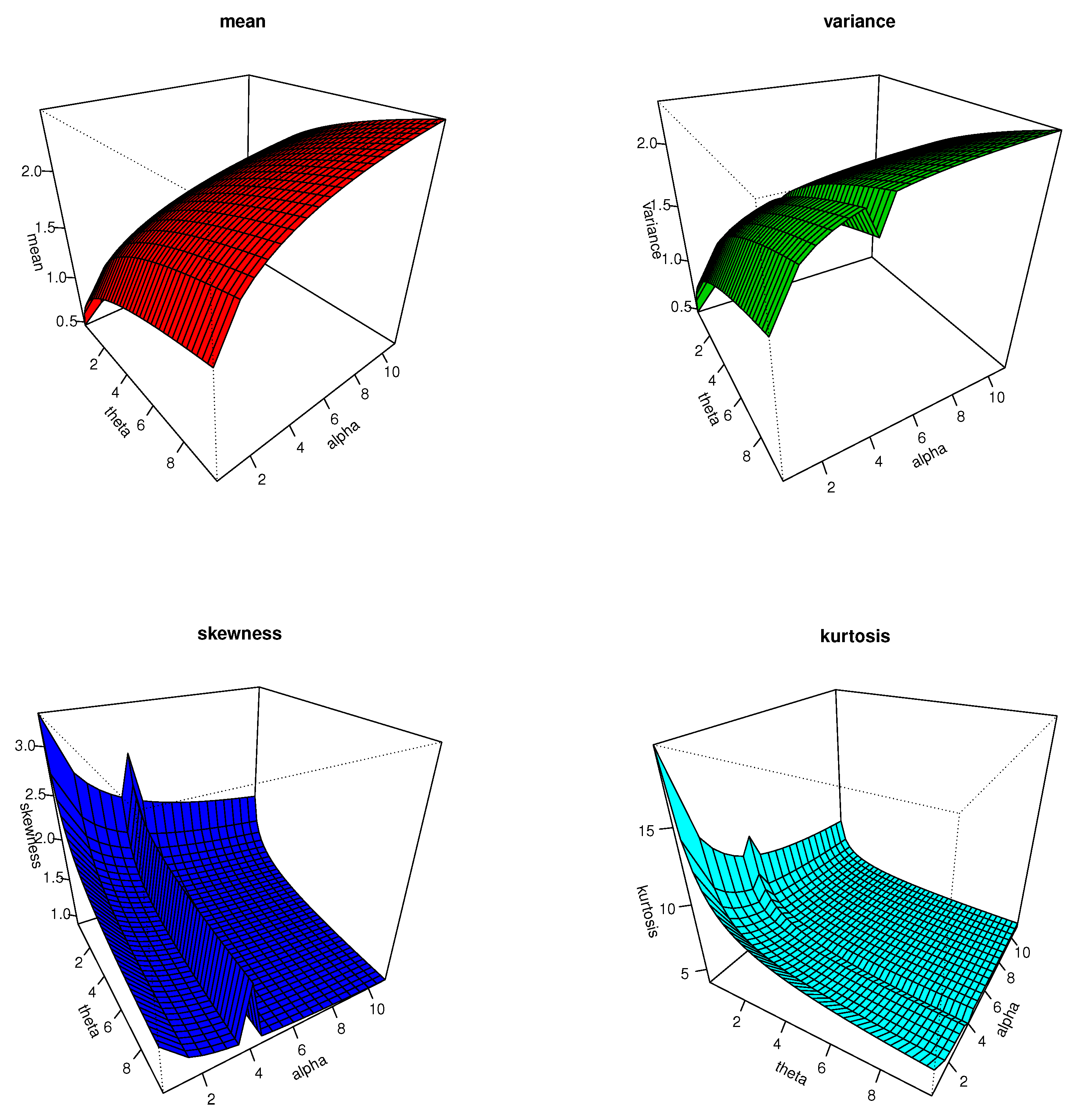
Using (24) and for different values for and with scale parameter , Figure 3 shows the plots for the mean, variance, skewness and kurtosis of the LTAPEx distribution. It is observed from Figure 3 that the mean and variance of the LTAPEx distribution increased as and increased. On the other hand, as and increased, the skewness and kurtosis decreased. It is also noted that the LTAPEx distribution is always a positively skewed distribution.
4.3. Entropies
Entropy has been employed in various cases and has numerous applications in different areas such as statistics and physics. For the random variable X, entropy measures uncertainty. The Rényi entropy (RE) is specified as follows.
From the LTAPEx distribution and using (7), we can write as follows.
Using series , the power series and the binomial expansion, we can write (27) as follows:
where the following is the case.
After simplification, Equation (30) becomes the following.
Another measure for entropy is the -entropy, which is obtained as follows.
Then, it follows from (28) that the following is obtained.
4.4. Order Statistics
Let refer to the order statistics of a random sample of size n taken from a continuous probability distribution with PDF and CDF , then the PDF of the sth order statistic, , can be expressed as follows:
where the following is the case.
For the LTAPEx distribution with CDF and PDF given by (14) and (15), respectively, and based on (33), we can write the PDF of the sth order statistic as follows:
where the following is the case.
Moreover, the CDF of the sth order statistic can be expressed as follows.
5. Estimation of the Parameters and Reliability Function
In this section, we consider the maximum likelihood estimation method for estimating parameters and as well as the reliability function of the LTAPEx distribution. Let be a random sample obtained from the LTAPEx distribution with PDF given by (15), then the likelihood function can be formulated as follows.
Taking the natural logarithm of (37), one can obtain the log-likelihood function, denoted by , as follows.
Hence, the maximum likelihood estimates (MLEs) of and , denoted by and , can be computed by maximizing the objective log-likelihood function in (38) with respect to and . Another useful approach to obtain these estimates is to solve the following three normal equations simultaneously.
It is observed from (39)–(41) that there are no ended forms for the MLEs of and . Therefore, to reach these estimates, we should adopt an iterative procedure for determining the numerical solution of (39)–(41). Now, based on the invariance property of MLEs, the MLEs of the RF at can be computed from (16) as follows.
The ACIs of and are instantly obtained based on the asymptotic properties of the MLEs. It is known that , where is the asymptotic variance–covariance matrix of MLEs. Actually, it is not easy to reach ; hence, the approximate asymptotic variance–covariance matrix of the MLEs expressed by can be used alternatively as follows
The elements and are the second derivatives of the log-likelihood function in (38), and they can be expressed as follows:
where , and . Now, the ACIs of parameters and can be computed as follows:
where is the upper th percentile point of the standard normal distribution.
In order to obtain the ACIs of the reliability function, we are required to obtain its variance. One of the common significant adopted procedures for approximating the variance is the delta method. To practice this approach, suppose that , where the following is the case:
where . Then, the approximate estimate for the variance of the reliability function is as follows, respectively:
Therefore, the two-sided ACI for the reliability function is provided by the following.
6. Simulation Study
In this section, a simulation analysis is accomplished to assess the performance of the MLEs of the unknown parameters and the reliability function. The efficiency of the estimates is evaluated using their mean squared errors (MSEs) and the confidence interval lengths. We employ Equation (22) to yield samples from the LTAPEx distribution. The simulation experiment is replicated 1000 times, each for samples of 25, 50 and 100. These sample sizes are selected to reflect the impact of small, intermediate and large sample sizes on the estimates. Moreover, different values for the unknown parameters and are considered. The selected values are , and . In a separate setting, we have acquired the MLE, MSE and confidence interval lengths (CILs). The simulation study is carried out based on following the steps:
- Decide the values of and the distinct time ;
- Generate n observations from the LTAPEx distribution using (22);
- Use the generated sample to compute the MLEs of , and ;
- Obtain the MSEs of , and ;
- Obtain the confidence interval bounds of , and ;
- Redo steps 2–5 M times;
- Compute the the average values (AVs) of MLEs, MSEs, confidence interval bounds (CIBs) and CILs of the parameter as follows:where and are the lower and upper CIBs, respectively.
The simulation outcomes are presented in Table 1, Table 2, Table 3, Table 4, Table 5 and Table 6. From these Tables, we can observe that as the sample size grows, the AV-MLEs of the different parameters and the reliability function are stable and relatively close to the actual parameter values. This implies that the MLEs act asymptotically unbiased estimators. Furthermore, the AV-MSEs reduce as the sample size increases in all issues, which indicate that the MLEs are consistent. Finally, one can observe that, as the sample size increases, CILs decrease in all the cases, as expected. This is because as the sample size raises, more additional information is collected.
7. Real Data Analysis
In this section, one real dataset is considered to explain the flexibility of our offered LTAPEx distribution. We compare the results of the LTAPEx distribution with some competitive distributions, such as exponential (Ex), generalized exponential (GEx) by Gupta and Kundu [24], APEx by Mahdavi and Kundu [8], APW by Nassar et al. [17] and Marshall–Olkin alpha power exponential (MOAPEx) by Nassar et al. [9]. The PDFs of these distributions are shown in Table 7 (for ). To compare the suitability of the different competitive models to fit the real datasets, we consider employing some different statistics including the following: The log-likelihood function is evaluated at the MLEs , Anderson–Darling () and Cramér–Von Mises (). Moreover, we use the Kolmogorov–Smirnov (KS) statistic in addition to the corresponding p-value.
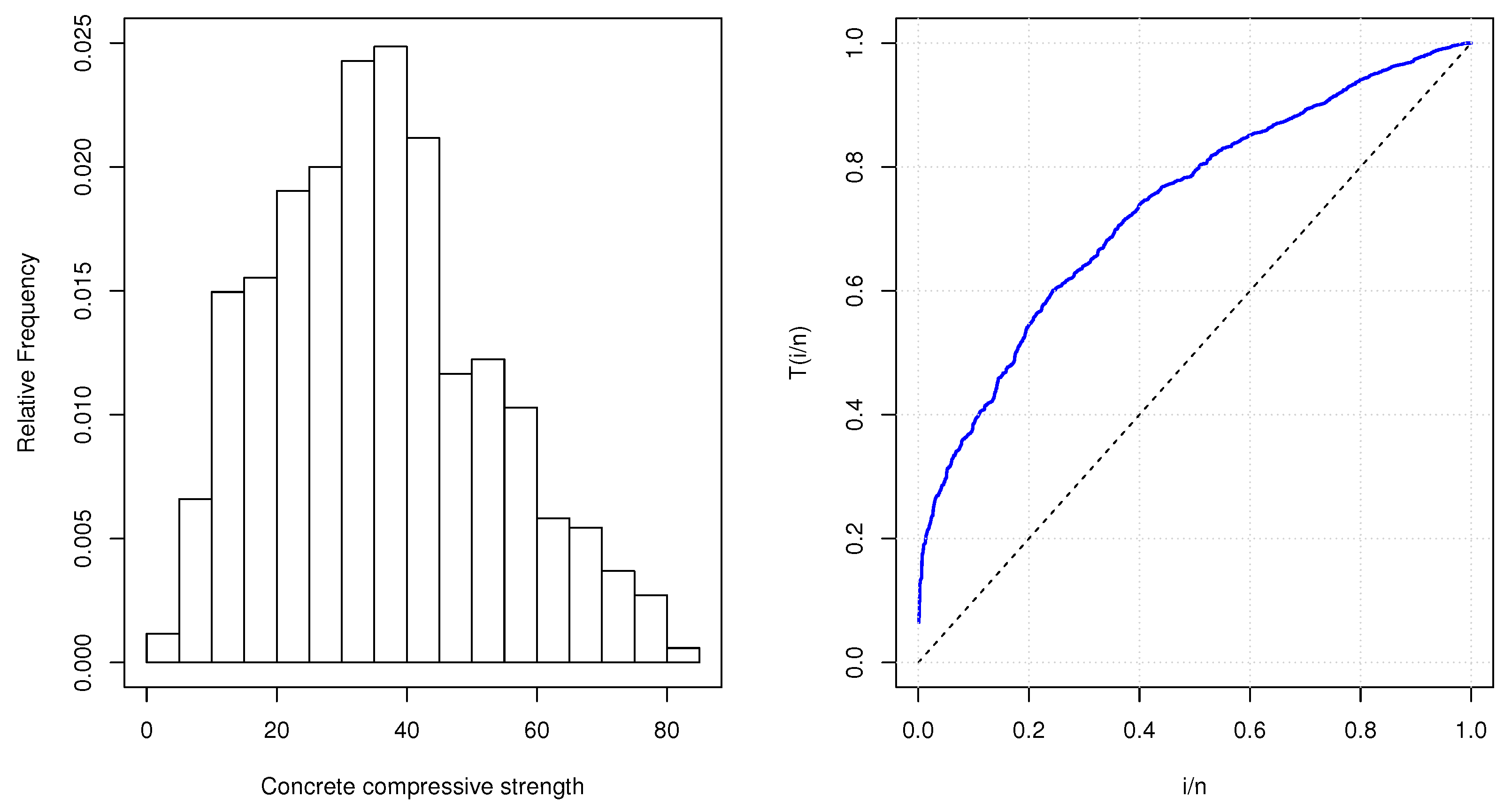
The dataset presents the high-performance concrete compressive strength, which is originally provided by Yeh [25] and analyzed recently by Alam and Nassar [26]. The dataset was established from 17 various sources to inspect the reliability of a proposed strength model. The data collected concrete comprising cement alongside fly ash, blast furnace slag and superplasticizer. The dataset consisted of a single dependent variable, namely the compressive strength of concrete (in MPa), and eight independent variables. The data contain 1030 instances. Our purpose here is to find a suitable model to fit the compressive strength of the concrete variable in order to evaluate reliability using some concrete compressive strength. Before analyzing this dataset, we first plot the corresponding histogram as well as the TTT plot. Figure 4 shows the corresponding histogram and the TTT plot. From this Figure, we can notice that the dataset is positively skewed. Furthermore, the TTT plot demonstrates that the empirical hazard rate function is an increasing function. Consequently, we can conclude that the LTAPEx distribution is appropriate to model this dataset.
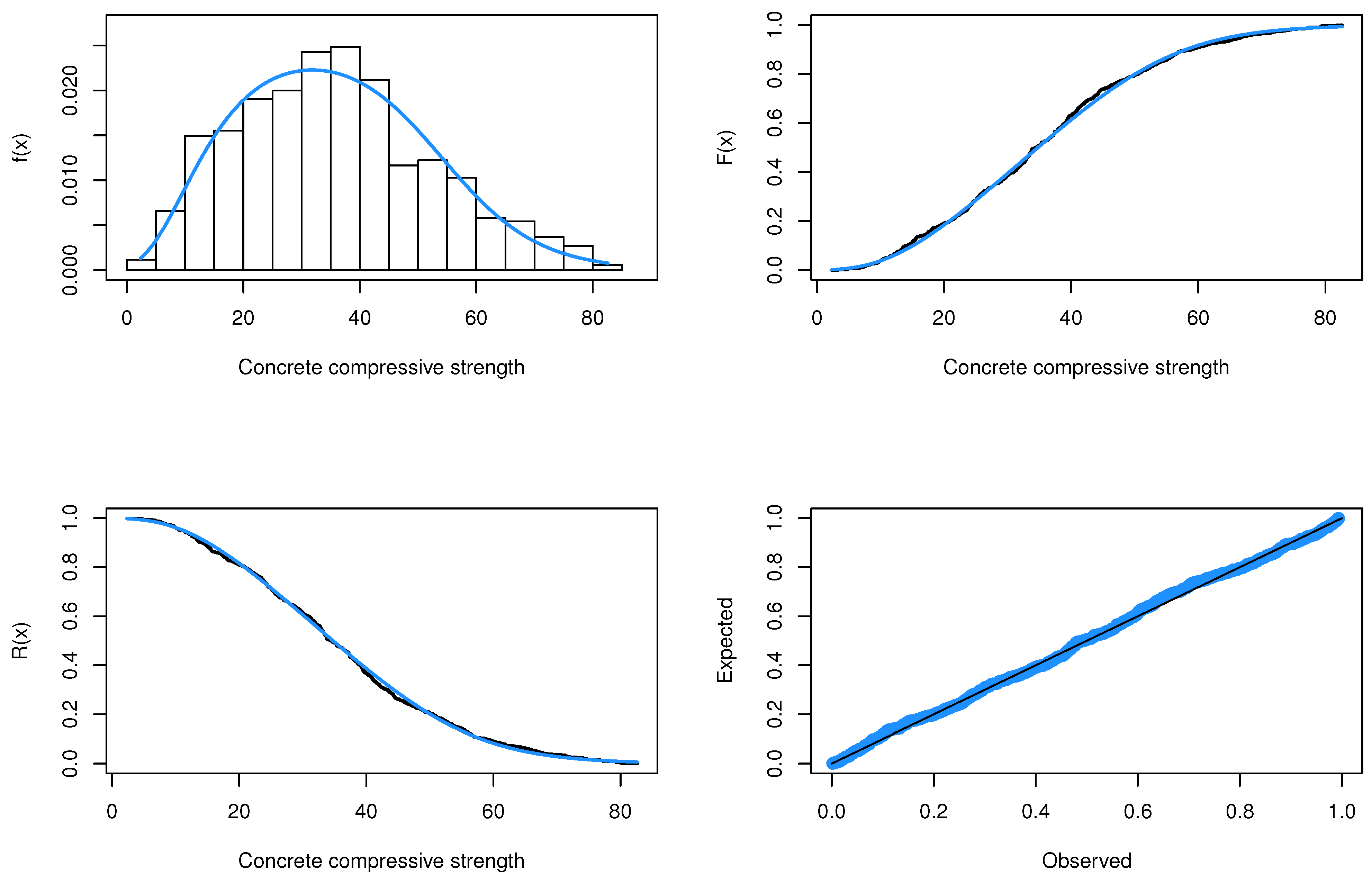
The MLEs of the unknown parameters of the LTAPEx model and the other competitive models are obtained and displayed in Table 8. Moreover, the standard errors and the different goodness-of-fit statistics are computed and presented also in Table 8. From Table 8, one can observe that the LTAPEx model has the lowest values of , and KS distance with the highest p-value compared to all other competitive models. Consequently, we can deduce that the LTAPEx model is the most acceptable model to fit concrete compressive strength data. Figure 5 shows the fitted density and the estimated CDF, RF and probability–probability (PP) plots of the LTAPEx model for concrete compressive strength data. Figure 5 demonstrates that the LTAPEx model can deliver a tight fit to the dataset. Generally, we can infer that the LTAPEx model is appropriate for modeling concrete compressive strength data rather than some traditional and some recently proposed distributions.
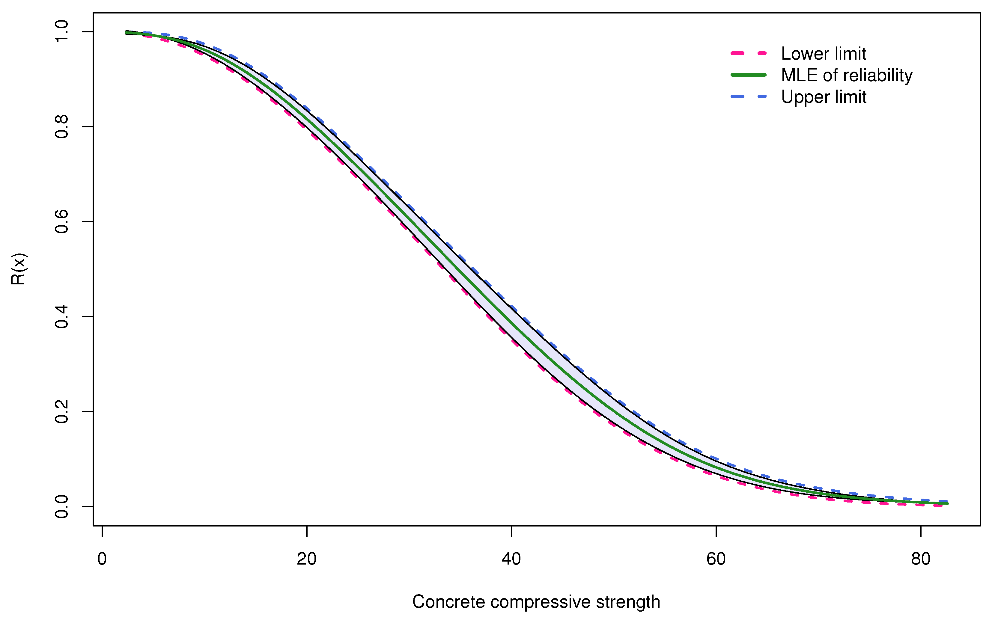
Practically, the concrete compressive strength can vary from 17 MPa to 28 MPa for residential constructions, while it can be increased as 70 MPa in the case of commercial buildings. Accordingly, based on the results of the LTAPEx distribution in Table 8, reliability is estimated at 17 MPa, 28 MPa and 70 MPa. Table 9 shows the input and output values of the proposed model. The different estimates and the associated CIBs are displayed in Table 10. Figure 6 shows the ACIs of the reliability function at each point of the real dataset. Based on the reliability probabilities displayed in Table 10, one can infer that the tested instances were appropriate for commercial constructions.
8. Conclusions
In this article, we have presented a new family of probability distributions called the logarithmic transformed alpha power family. The new family is obtained by taking the distribution function of the well-known alpha power method as the baseline distribution in the logarithmic transformed method. Some structural properties of the new family are derived. We have used the offered family to introduce a new three-parameter exponential distribution. We refer to the proposed distribution as the logarithmic transformed alpha power exponential distribution. The point and interval estimates of the unknown parameters and the reliability function are obtained via the maximum likelihood estimation method. By conducting a simulation study, the behavior of the point and interval estimates is studied based on mean square errors and confidence interval lengths, respectively. Moreover, one application relative to the high-performance concrete compressive strength dataset is considered. Based on theoretical and numerical results, we can conclude the following:
- The new distribution is able to provide a better fit for high-performance concrete compressive strength data rather than some other competitive distributions.
- The hazard rate function of the proposed model can bear various forms including decreasing, increasing, upside-down bathtub and bathtub-shaped rates.
- The proposed model can be regarded to be effective in modeling lifetime data.
- The simulation outcomes demonstrated that the estimates are asymptotically unbiased and consistent.
- The confidence interval of the reliability function performs well in terms of confidence length, which indicates that the delta method produces a small variation.
- Based on the empirical outcomes, we can infer that the logarithmic-transformed alpha power exponential distribution delivers a more satisfactory fit to the high-performance concrete compressive strength data than the traditional exponential and some other competitive models.
- As a future work, it is of interest to consider the same model described in this paper to assess the reliability of normal concrete.
Author Contributions
Investigation, R.A. and M.N.; methodology, M.N. and R.A.; software, M.N.; validation, R.A. and M.N.; funding acquisition, R.A.; writing, M.N. and R.A. All authors have read and agreed to the published version of the manuscript.
Funding
Princess Nourah bint Abdulrahman University Researchers Supporting Project number (PNURSP2022R50), Princess Nourah bint Abdulrahman University, Riyadh, Saudi Arabia.
Institutional Review Board Statement
Not applicable.
Informed Consent Statement
Not applicable.
Data Availability Statement
Three datasets are contained within the article.
Acknowledgments
The authors would like to express their thanks to the editor and anonymous referees for useful suggestions and valuable comments. This work was funded by Princess Nourah bint Abdulrahman University Researchers Supporting Project number (PNURSP2022R50), Princess Nourah bint Abdulrahman University, Riyadh, Saudi Arabia.
Conflicts of Interest
The authors declare no conflict of interest.
References
- Mudholkar, G.S.; Srivastava, D.K. Exponentiated Weibull family for analyzing bathtub failure-rate data. IEEE Trans. Reliab. 1993, 42, 299–302. [Google Scholar] [CrossRef]
- Marshall, A.W.; Olkin, I. A new method for adding a parameter to a family of distributions with application to the exponential and Weibull families. Biometrika 1997, 84, 641–652. [Google Scholar] [CrossRef]
- Eugene, N.; Lee, C.; Famoye, F. Beta-normal distribution and its applications. Commun. Stat.-Theory Methods 2002, 31, 497–512. [Google Scholar] [CrossRef]
- Cordeiro, G.M.; de Castro, M. A new family of generalized distributions. J. Stat. Comput. Simul. 2011, 81, 883–898. [Google Scholar] [CrossRef]
- Alzaatreh, A.; Lee, C.; Famoye, F. A new method for generating families of continuous distributions. Metron 2013, 71, 63–79. [Google Scholar] [CrossRef] [Green Version]
- Bourguignon, M.; Silva, R.B.; Cordeiro, G.M. The Weibull-G family of probability distributions. J. Data Sci. 2014, 12, 53–68. [Google Scholar] [CrossRef]
- Pappas, V.; Adamidis, K.; Loukas, S. A family of lifetime distributions. J. Qual. Reliab. Eng. 2012, 2012, 760687. [Google Scholar] [CrossRef] [Green Version]
- Mahdavi, A.; Kundu, D. A new method for generating distributions with an application to exponential distribution. Commun. Stat.-Theory Methods 2017, 46, 6543–6557. [Google Scholar] [CrossRef]
- Nassar, M.; Kumar, D.; Dey, S.; Cordeiro, G.M.; Afify, A.Z. The Marshall–Olkin alpha power family of distributions with applications. J. Comput. Appl. Math. 2019, 351, 41–53. [Google Scholar] [CrossRef]
- Alotaibi, R.; Okasha, H.; Rezk, H.; Nassar, M. A new weighted version of alpha power transformation method: Properties and applications to COVID-19 and software reliability data. Phys. Scr. 2021, 96, 125221. [Google Scholar] [CrossRef]
- Lee, C.; Famoye, F.; Alzaatreh, A.Y. Methods for generating families of univariate continuous distributions in the recent decades. Wiley Interdiscip. Rev. Comput. Stat. 2013, 5, 219–238. [Google Scholar] [CrossRef]
- Jones, M.C. On families of distributions with shape parameters. Int. Stat. Rev. 2015, 83, 175–192. [Google Scholar] [CrossRef]
- Xie, M.; Tang, Y.; Goh, T.N. A modified Weibull extension with bathtub-shaped failure rate function. Reliab. Eng. Syst. Saf. 2002, 76, 279–285. [Google Scholar] [CrossRef]
- Nassar, M.; Afify, A.Z.; Dey, S.; Kumar, D. A new extension of Weibull distribution: Properties and different methods of estimation. J. Comput. Appl. Math. 2018, 336, 439–457. [Google Scholar] [CrossRef]
- Eltehiwy, M. Logarithmic inverse Lindley distribution: Model, properties and applications. J. King Saud Univ.-Sci. 2020, 32, 136–144. [Google Scholar] [CrossRef]
- Alotaibi, R.; Okasha, H.; Rezk, H.; Almarashi, A.M.; Nassar, M. On a new flexible Lomax distribution: Statistical properties and estimation procedures with applications to engineering and medical data. AIMS Math. 2021, 6, 13976–13999. [Google Scholar] [CrossRef]
- Nassar, M.; Alzaatreh, A.; Mead, M.; Abo-Kasem, O. Alpha power Weibull distribution: Properties and applications. Commun. Stat.-Theory Methods 2017, 46, 10236–10252. [Google Scholar] [CrossRef]
- Dey, S.; Nassar, M.; Kumar, D. Alpha power transformed inverse Lindley distribution: A distribution with an upside-down bathtub-shaped hazard function. J. Comput. Appl. Math. 2019, 348, 130–145. [Google Scholar] [CrossRef]
- Ihtisham, S.; Khalil, A.; Manzoor, S.; Khan, S.A.; Ali, A. Alpha-Power Pareto distribution: Its properties and applications. PLoS ONE 2019, 14, e0218027. [Google Scholar] [CrossRef]
- Eghwerido, J.T.; Nzei, L.C.; Agu, F.I. The alpha power Gompertz distribution: Characterization, properties, and applications. Sankhya A 2020, 83, 449–475. [Google Scholar] [CrossRef]
- Eghwerido, J.T. The alpha power Teissier distribution and its applications. Afr. Stat. 2021, 16, 2733–2747. [Google Scholar] [CrossRef]
- Eghwerido, J.T.; Nzei, L.C.; Zelibe, S.C. The alpha power extended generalized exponential distribution. J. Stat. Manag. Syst. 2021, 25, 187–210. [Google Scholar] [CrossRef]
- Dey, S.; Nassar, M.; Kumar, D. α Logarithmic Transformed Family of Distributions with Application. Ann. Data Sci. 2017, 4, 457–482. [Google Scholar] [CrossRef]
- Gupta, R.D.; Kundu, D. Theory & methods: Generalized exponential distributions. Aust. N. Z. J. Stat. 1999, 41, 173–188. [Google Scholar]
- Yeh, I.C. Modeling of strength of high-performance concrete using artificial neural networks. Cem. Concr. Res. 1998, 28, 1797–1808. [Google Scholar] [CrossRef]
- Alam, F.M.A.; Nassar, M. On Modeling Concrete Compressive Strength Data Using Laplace Birnbaum-Saunders Distribution Assuming Contaminated Information. Crystals 2021, 11, 830. [Google Scholar] [CrossRef]
Figure 1.
Different plots of the PDF of the LTAPEx distribution for various values of and with .

Figure 2.
Different plots of the HRF of the LTAPEx distribution for various values of and with .

Figure 3.
Mean, variance, skewness and kurtosis of LTAPEx distribution.

Figure 4.
Histogram and TTT plots for the concrete compressive strength data.

Figure 5.
Plots of fitted functions and PP plot of the LTAPEx distribution for concrete compressive strength data.
Figure 5.
Plots of fitted functions and PP plot of the LTAPEx distribution for concrete compressive strength data.

Figure 6.
The ACIs of for the concrete compressive strength data.


Table 1.
The AVs of estimates and the corresponding MSEs for .
| Parameters | B | MSE | ||||||||
|---|---|---|---|---|---|---|---|---|---|---|
| 0.5 | 0.5 | 0.5 | 0.694 | 0.670 | 0.648 | 0.592 | 0.347 | 0.343 | 0.149 | 0.033 |
| 1.0 | 0.698 | 0.699 | 1.290 | 0.409 | 0.390 | 0.401 | 0.576 | 0.037 | ||
| 1.5 | 0.684 | 0.716 | 1.938 | 0.302 | 0.335 | 0.432 | 1.319 | 0.033 | ||
| 2.5 | 0.665 | 0.673 | 3.249 | 0.173 | 0.275 | 0.366 | 3.789 | 0.022 | ||
| 5.0 | 0.687 | 0.672 | 6.455 | 0.064 | 0.314 | 0.329 | 14.69 | 0.008 | ||
| 1.5 | 0.5 | 0.634 | 2.380 | 0.608 | 0.702 | 0.371 | 5.619 | 0.096 | 0.026 | |
| 1.0 | 0.590 | 1.945 | 1.221 | 0.511 | 0.290 | 2.865 | 0.385 | 0.037 | ||
| 1.5 | 0.585 | 2.198 | 1.823 | 0.398 | 0.257 | 4.563 | 0.817 | 0.038 | ||
| 2.5 | 0.617 | 2.133 | 3.054 | 0.251 | 0.298 | 4.129 | 2.490 | 0.031 | ||
| 5.0 | 0.605 | 2.056 | 6.050 | 0.093 | 0.275 | 3.494 | 9.092 | 0.014 | ||
| 2.5 | 0.5 | 0.574 | 3.970 | 0.600 | 0.736 | 0.261 | 16.93 | 0.076 | 0.023 | |
| 1.0 | 0.537 | 4.069 | 1.196 | 0.557 | 0.211 | 18.60 | 0.301 | 0.043 | ||
| 1.5 | 0.599 | 3.960 | 1.793 | 0.441 | 0.347 | 17.21 | 0.696 | 0.042 | ||
| 2.5 | 0.575 | 4.080 | 2.986 | 0.283 | 0.270 | 18.04 | 1.897 | 0.039 | ||
| 5.0 | 0.559 | 3.822 | 6.005 | 0.107 | 0.247 | 15.24 | 8.021 | 0.020 | ||
| 1.5 | 0.5 | 0.5 | 1.619 | 0.779 | 0.651 | 0.685 | 1.371 | 0.599 | 0.145 | 0.029 |
| 1.0 | 1.597 | 0.833 | 1.299 | 0.502 | 1.408 | 0.752 | 0.562 | 0.044 | ||
| 1.5 | 1.623 | 0.796 | 1.950 | 0.389 | 1.364 | 0.607 | 1.335 | 0.045 | ||
| 2.5 | 1.593 | 0.779 | 3.275 | 0.233 | 1.292 | 0.628 | 3.834 | 0.033 | ||
| 5.0 | 1.581 | 0.773 | 6.493 | 0.088 | 1.327 | 0.559 | 14.29 | 0.015 | ||
| 1.5 | 0.5 | 1.688 | 2.136 | 0.629 | 0.768 | 2.385 | 4.508 | 0.101 | 0.021 | |
| 1.0 | 1.727 | 2.167 | 1.262 | 0.600 | 2.786 | 4.855 | 0.384 | 0.039 | ||
| 1.5 | 1.609 | 1.964 | 1.899 | 0.460 | 2.328 | 3.382 | 0.911 | 0.049 | ||
| 2.5 | 1.736 | 2.178 | 3.153 | 0.305 | 2.963 | 4.519 | 2.489 | 0.042 | ||
| 5.0 | 1.673 | 2.038 | 6.354 | 0.109 | 2.421 | 3.808 | 10.53 | 0.017 | ||
| 2.5 | 0.5 | 1.665 | 3.143 | 0.632 | 0.798 | 2.987 | 8.055 | 0.097 | 0.016 | |
| 1.0 | 1.522 | 3.336 | 1.253 | 0.650 | 1.480 | 9.600 | 0.379 | 0.031 | ||
| 1.5 | 1.578 | 3.070 | 1.878 | 0.506 | 2.207 | 7.305 | 0.820 | 0.046 | ||
| 2.5 | 1.493 | 3.280 | 3.148 | 0.332 | 1.324 | 8.840 | 2.293 | 0.041 | ||
| 5.0 | 1.579 | 3.262 | 6.276 | 0.114 | 2.248 | 8.689 | 9.034 | 0.015 | ||
Table 2.
The AVs of estimates and the corresponding MSEs for .
| Parameters | MLE | MSE | ||||||||
|---|---|---|---|---|---|---|---|---|---|---|
| 0.5 | 0.5 | 0.5 | 0.636 | 0.631 | 0.556 | 0.657 | 0.119 | 0.115 | 0.059 | 0.015 |
| 1.0 | 0.622 | 0.609 | 1.114 | 0.460 | 0.102 | 0.096 | 0.240 | 0.021 | ||
| 1.5 | 0.596 | 0.622 | 1.680 | 0.336 | 0.069 | 0.096 | 0.525 | 0.018 | ||
| 2.5 | 0.607 | 0.619 | 2.784 | 0.198 | 0.078 | 0.092 | 1.458 | 0.015 | ||
| 5.0 | 0.608 | 0.618 | 5.584 | 0.068 | 0.077 | 0.094 | 6.716 | 0.007 | ||
| 1.5 | 0.5 | 0.658 | 1.656 | 0.551 | 0.750 | 0.152 | 0.659 | 0.038 | 0.008 | |
| 1.0 | 0.621 | 1.728 | 1.102 | 0.573 | 0.110 | 0.928 | 0.160 | 0.017 | ||
| 1.5 | 0.648 | 1.695 | 1.652 | 0.447 | 0.149 | 0.727 | 0.346 | 0.021 | ||
| 2.5 | 0.662 | 1.642 | 2.744 | 0.279 | 0.163 | 0.647 | 0.926 | 0.021 | ||
| 5.0 | 0.632 | 1.642 | 5.504 | 0.094 | 0.125 | 0.643 | 3.658 | 0.009 | ||
| 2.5 | 0.5 | 0.570 | 2.997 | 0.552 | 0.790 | 0.077 | 3.055 | 0.032 | 0.006 | |
| 1.0 | 0.576 | 2.938 | 1.106 | 0.623 | 0.086 | 2.883 | 0.127 | 0.014 | ||
| 1.5 | 0.584 | 2.849 | 1.649 | 0.492 | 0.094 | 2.685 | 0.284 | 0.019 | ||
| 2.5 | 0.581 | 2.919 | 2.777 | 0.309 | 0.089 | 2.768 | 0.830 | 0.019 | ||
| 5.0 | 0.611 | 2.803 | 5.525 | 0.107 | 0.133 | 1.878 | 3.259 | 0.010 | ||
| 1.5 | 0.5 | 0.5 | 1.816 | 0.584 | 0.571 | 0.744 | 0.818 | 0.089 | 0.053 | 0.010 |
| 1.0 | 1.818 | 0.560 | 1.140 | 0.563 | 0.766 | 0.068 | 0.207 | 0.019 | ||
| 1.5 | 1.821 | 0.582 | 1.713 | 0.437 | 0.746 | 0.097 | 0.471 | 0.023 | ||
| 2.5 | 1.831 | 0.576 | 2.847 | 0.271 | 0.837 | 0.092 | 1.289 | 0.023 | ||
| 5.0 | 1.824 | 0.567 | 5.694 | 0.095 | 0.768 | 0.078 | 5.130 | 0.011 | ||
| 1.5 | 0.5 | 1.771 | 1.652 | 0.575 | 0.824 | 0.941 | 0.581 | 0.032 | 0.004 | |
| 1.0 | 1.874 | 1.752 | 1.147 | 0.677 | 1.378 | 1.037 | 0.126 | 0.011 | ||
| 1.5 | 1.761 | 1.728 | 1.722 | 0.545 | 0.921 | 0.885 | 0.286 | 0.016 | ||
| 2.5 | 1.722 | 1.635 | 2.869 | 0.348 | 0.799 | 0.536 | 0.780 | 0.018 | ||
| 5.0 | 1.817 | 1.653 | 5.755 | 0.118 | 1.148 | 0.593 | 3.269 | 0.010 | ||
| 2.5 | 0.5 | 1.807 | 2.932 | 0.579 | 0.859 | 1.249 | 2.651 | 0.027 | 0.003 | |
| 1.0 | 1.883 | 2.873 | 1.160 | 0.723 | 1.544 | 2.413 | 0.111 | 0.008 | ||
| 1.5 | 1.776 | 2.837 | 1.744 | 0.596 | 1.130 | 2.013 | 0.252 | 0.013 | ||
| 2.5 | 1.855 | 2.858 | 2.912 | 0.397 | 1.421 | 2.251 | 0.726 | 0.018 | ||
| 5.0 | 1.739 | 2.884 | 5.817 | 0.129 | 0.930 | 2.396 | 2.957 | 0.007 | ||
Table 3.
The AVs of estimates and the corresponding MSEs for .
| Parameters | MLE | MSE | ||||||||
|---|---|---|---|---|---|---|---|---|---|---|
| 0.5 | 0.5 | 0.5 | 0.586 | 0.521 | 0.515 | 0.650 | 0.058 | 0.016 | 0.027 | 0.010 |
| 1.0 | 0.573 | 0.523 | 1.026 | 0.458 | 0.048 | 0.016 | 0.109 | 0.015 | ||
| 1.5 | 0.572 | 0.523 | 1.537 | 0.337 | 0.045 | 0.016 | 0.247 | 0.016 | ||
| 2.5 | 0.576 | 0.521 | 2.589 | 0.193 | 0.048 | 0.016 | 0.677 | 0.013 | ||
| 5.0 | 0.569 | 0.528 | 5.147 | 0.066 | 0.045 | 0.021 | 2.785 | 0.007 | ||
| 1.5 | 0.5 | 0.568 | 1.581 | 0.521 | 0.757 | 0.033 | 0.174 | 0.022 | 0.004 | |
| 1.0 | 0.560 | 1.589 | 1.048 | 0.577 | 0.033 | 0.198 | 0.084 | 0.010 | ||
| 1.5 | 0.557 | 1.565 | 1.573 | 0.445 | 0.028 | 0.119 | 0.189 | 0.012 | ||
| 2.5 | 0.550 | 1.573 | 2.620 | 0.272 | 0.028 | 0.136 | 0.552 | 0.013 | ||
| 5.0 | 0.553 | 1.609 | 5.223 | 0.092 | 0.033 | 0.196 | 2.086 | 0.009 | ||
| 2.5 | 0.5 | 0.523 | 2.586 | 0.544 | 0.785 | 0.017 | 0.525 | 0.015 | 0.002 | |
| 1.0 | 0.526 | 2.545 | 1.085 | 0.613 | 0.019 | 0.428 | 0.062 | 0.006 | ||
| 1.5 | 0.522 | 2.559 | 1.624 | 0.478 | 0.018 | 0.587 | 0.134 | 0.008 | ||
| 2.5 | 0.536 | 2.592 | 2.729 | 0.291 | 0.021 | 0.567 | 0.382 | 0.008 | ||
| 5.0 | 0.526 | 2.614 | 5.471 | 0.085 | 0.017 | 0.606 | 1.490 | 0.003 | ||
| 1.5 | 0.5 | 0.5 | 1.714 | 0.515 | 0.535 | 0.749 | 0.439 | 0.012 | 0.033 | 0.007 |
| 1.0 | 1.741 | 0.520 | 1.064 | 0.576 | 0.452 | 0.012 | 0.133 | 0.015 | ||
| 1.5 | 1.563 | 0.519 | 1.595 | 0.439 | 0.128 | 0.010 | 0.297 | 0.018 | ||
| 2.5 | 1.560 | 0.512 | 2.669 | 0.267 | 0.128 | 0.012 | 0.813 | 0.019 | ||
| 5.0 | 1.561 | 0.518 | 5.301 | 0.098 | 0.131 | 0.012 | 3.306 | 0.013 | ||
| 1.5 | 0.5 | 1.555 | 1.483 | 0.563 | 0.822 | 0.109 | 0.034 | 0.020 | 0.002 | |
| 1.0 | 1.553 | 1.480 | 1.129 | 0.664 | 0.104 | 0.060 | 0.082 | 0.006 | ||
| 1.5 | 1.548 | 1.488 | 1.690 | 0.534 | 0.086 | 0.067 | 0.175 | 0.009 | ||
| 2.5 | 1.538 | 1.493 | 2.804 | 0.339 | 0.087 | 0.045 | 0.473 | 0.010 | ||
| 5.0 | 1.539 | 1.473 | 5.615 | 0.102 | 0.086 | 0.042 | 1.848 | 0.004 | ||
| 2.5 | 0.5 | 1.527 | 2.509 | 0.565 | 0.857 | 0.061 | 0.143 | 0.018 | 0.001 | |
| 1.0 | 1.528 | 2.524 | 1.122 | 0.722 | 0.043 | 0.205 | 0.064 | 0.004 | ||
| 1.5 | 1.519 | 2.518 | 1.687 | 0.595 | 0.049 | 0.191 | 0.149 | 0.007 | ||
| 2.5 | 1.522 | 2.499 | 2.807 | 0.390 | 0.047 | 0.154 | 0.399 | 0.009 | ||
| 5.0 | 1.525 | 2.521 | 5.608 | 0.122 | 0.046 | 0.191 | 1.571 | 0.004 | ||
Table 4.
The AVs of CIBs (in parentheses) and the corresponding CILs for .
| Parameters | ACIs | |||||
|---|---|---|---|---|---|---|
| 0.5 | 0.5 | 0.5 | [0,2.746]2.746 | [0,2.916]2.916 | [0.050,1.247]1.196 | [0.422,0.761]0.338 |
| 1.0 | [0,2.510]2.510 | [0,2.945]2.945 | [0.263,2.316]2.053 | [0.254,0.564]0.310 | ||
| 1.5 | [0,2.602]2.602 | [0,3.159]3.159 | [0.215,3.662]3.447 | [0.163,0.441]0.278 | ||
| 2.5 | [0,2.502]2.502 | [0,2.974]2.974 | [0.531,5.967]5.436 | [0.082,0.264]0.182 | ||
| 5.0 | [0,2.523]2.523 | [0,2.908]2.908 | [0.877,12.04]11.15 | [0.013,0.115]0.102 | ||
| 1.5 | 0.5 | [0,3.160]3.160 | [0,11.24]11.24 | [0.271,0.945]0.674 | [0.566,0.838]0.272 | |
| 1.0 | [0,3.038]3.038 | [0,10.07]10.07 | [0.461,1.980]1.519 | [0.343,0.679]0.336 | ||
| 1.5 | [0,2.814]2.814 | [0,10.38]10.38 | [0.742,2.905]2.163 | [0.247,0.549]0.302 | ||
| 2.5 | [0,2.885]2.885 | [0,9.831]9.831 | [1.264,4.844]3.580 | [0.144,0.357]0.213 | ||
| 5.0 | [0,2.833]2.833 | [0,9.796]9.796 | [2.287,9.812]7.525 | [0.034,0.153]0.119 | ||
| 2.5 | 0.5 | [0,1.982]1.982 | [0,16.45]16.45 | [0.248,0.952]0.704 | [0.588,0.884]0.296 | |
| 1.0 | [0,1.739]1.739 | [0,15.49]15.49 | [0.536,1.855]1.319 | [0.410,0.704]0.294 | ||
| 1.5 | [0,1.872]1.872 | [0,15.85]15.85 | [0.920,2.666]1.747 | [0.297,0.586]0.288 | ||
| 2.5 | [0,1.823]1.823 | [0,15.90]15.90 | [1.467,4.505]3.039 | [0.172,0.394]0.222 | ||
| 5.0 | [0,1.793]1.793 | [0,15.01]15.01 | [2.863,9.148]6.285 | [0.047,0.167]0.120 | ||
| 1.5 | 0.5 | 0.5 | [0,5.296]5.296 | [0,2.951]2.951 | [0.231,1.071]0.839 | [0.554,0.817]0.263 |
| 1.0 | [0,5.235]5.235 | [0,3.156]3.156 | [0.479,2.119]1.640 | [0.350,0.654]0.304 | ||
| 1.5 | [0,5.366]5.366 | [0,3.082]3.082 | [0.678,3.221]2.543 | [0.247,0.530]0.283 | ||
| 2.5 | [0,5.269]5.269 | [0,2.997]2.997 | [1.150,5.399]4.249 | [0.128,0.338]0.209 | ||
| 5.0 | [0,5.160]5.160 | [0,2.970]2.970 | [2.426,10.560]8.13 | [0.035,0.141]0.106 | ||
| 1.5 | 0.5 | [0,5.380]5.380 | [0,7.637]7.637 | [0.283,0.976]0.692 | [0.666,0.870]0.203 | |
| 1.0 | [0,5.574]5.574 | [0,7.905]7.905 | [0.582,1.943]1.362 | [0.463,0.737]0.275 | ||
| 1.5 | [0,5.668]5.668 | [0,7.272]7.272 | [0.838,2.959]2.121 | [0.321,0.599]0.278 | ||
| 2.5 | [0,5.447]5.447 | [0,7.710]7.710 | [1.443,4.863]3.420 | [0.182,0.429]0.246 | ||
| 5.0 | [0,6.181]6.181 | [0,7.557]7.557 | [2.531,10.17]7.645 | [0.040,0.179]0.139 | ||
| 2.5 | 0.5 | [0,5.310]5.310 | [0,12.37]12.37 | [0.327,0.937]0.611 | [0.701,0.895]0.194 | |
| 1.0 | [0,4.956]4.956 | [0,12.34]12.34 | [0.656,1.849]1.193 | [0.516,0.784]0.268 | ||
| 1.5 | [0,5.045]5.045 | [0,11.89]11.89 | [0.940,2.816]1.876 | [0.361,0.650]0.289 | ||
| 2.5 | [0,4.763]4.763 | [0,12.48]12.48 | [1.660,4.636]2.975 | [0.199,0.465]0.266 | ||
| 5.0 | [0,4.915]4.915 | [0,13.08]13.08 | [3.292,9.261]5.969 | [0.038,0.191]0.153 | ||
Table 5.
The AVs of CIBs (in parentheses) and the corresponding CILs for .
| Parameters | ACIs | |||||
|---|---|---|---|---|---|---|
| 0.5 | 0.5 | 0.5 | [0,1.920]1.920 | [0,2.104]2.104 | [0.234,0.878]0.644 | [0.538,0.775]0.236 |
| 1.0 | [0,1.892]1.892 | [0,2.103]2.103 | [0.433,1.795]1.363 | [0.341,0.579]0.238 | ||
| 1.5 | [0,1.749]1.749 | [0,2.067]2.067 | [0.680,2.680]2.000 | [0.231,0.440]0.209 | ||
| 2.5 | [0,1.936]1.936 | [0,2.201]2.201 | [0.861,4.707]3.847 | [0.117,0.278]0.161 | ||
| 5.0 | [0,1.785]1.785 | [0,2.046]2.046 | [2.275,8.892]6.617 | [0.027,0.109]0.083 | ||
| 1.5 | 0.5 | [0,2.713]2.713 | [0,6.503]6.503 | [0.296,0.805]0.509 | [0.648,0.851]0.203 | |
| 1.0 | [0,2.781]2.781 | [0,6.918]6.918 | [0.599,1.606]1.007 | [0.457,0.689]0.233 | ||
| 1.5 | [0,2.778]2.778 | [0,6.921]6.921 | [0.853,2.452]1.600 | [0.329,0.566]0.237 | ||
| 2.5 | [0,2.967]2.967 | [0,6.832]6.832 | [1.440,4.048]2.608 | [0.181,0.377]0.195 | ||
| 5.0 | [0,2.912]2.912 | [0,6.876]6.876 | [2.873,8.134]5.261 | [0.037,0.151]0.114 | ||
| 2.5 | 0.5 | [0,1.854]1.854 | [0,9.675]9.675 | [0.315,0.789]0.474 | [0.691,0.888]0.197 | |
| 1.0 | [0,1.906]1.906 | [0,9.730]9.730 | [0.605,1.608]1.003 | [0.485,0.761]0.276 | ||
| 1.5 | [0,1.846]1.846 | [0,9.004]9.004 | [0.928,2.371]1.444 | [0.366,0.618]0.251 | ||
| 2.5 | [0,1.927]1.927 | [0,9.722]9.722 | [1.493,4.061]2.568 | [0.196,0.422]0.226 | ||
| 5.0 | [0,1.882]1.882 | [0,8.906]8.906 | [3.170,7.880]4.710 | [0.051,0.162]0.111 | ||
| 1.5 | 0.5 | 0.5 | [0,5.046]5.046 | [0,1.655]1.655 | [0.308,0.833]0.525 | [0.661,0.828]0.166 |
| 1.0 | [0,5.189]5.189 | [0,1.614]1.614 | [0.593,1.688]1.095 | [0.454,0.672]0.219 | ||
| 1.5 | [0,5.174]5.174 | [0,1.664]1.664 | [0.923,2.503]1.580 | [0.332,0.541]0.209 | ||
| 2.5 | [0,5.034]5.034 | [0,1.585]1.585 | [1.549,4.144]2.595 | [0.187,0.354]0.166 | ||
| 5.0 | [0,5.161]5.161 | [0,1.608]1.608 | [3.033,8.355]5.322 | [0.046,0.144]0.098 | ||
| 1.5 | 0.5 | [0,4.447]4.447 | [0,4.113]4.113 | [0.352,0.798]0.447 | [0.753,0.895]0.142 | |
| 1.0 | [0,4.603]4.603 | [0,4.239]4.239 | [0.736,1.559]0.823 | [0.582,0.772]0.190 | ||
| 1.5 | [0,4.344]4.344 | [0,4.188]4.188 | [1.098,2.347]1.249 | [0.441,0.650]0.209 | ||
| 2.5 | [0,4.391]4.391 | [0,4.093]4.093 | [1.730,4.007]2.277 | [0.246,0.450]0.203 | ||
| 5.0 | [0,4.619]4.619 | [0,4.198]4.198 | [3.590,7.920]4.330 | [0.057,0.179]0.122 | ||
| 2.5 | 0.5 | [0,4.818]4.818 | [0,8.072]8.072 | [0.361,0.798]0.436 | [0.790,0.927]0.137 | |
| 1.0 | [0,5.083]5.083 | [0,8.031]8.031 | [0.718,1.601]0.883 | [0.620,0.827]0.206 | ||
| 1.5 | [0,4.972]4.972 | [0,8.218]8.218 | [0.980,2.508]1.528 | [0.463,0.729]0.267 | ||
| 2.5 | [0,4.857]4.857 | [0,7.801]7.801 | [1.811,4.013]2.202 | [0.289,0.505]0.216 | ||
| 5.0 | [0,4.753]4.753 | [0,7.941]7.941 | [3.574,8.061]4.487 | [0.063,0.195]0.132 | ||
Table 6.
The AVs of CIBs (in parentheses) and the corresponding CILs for .
| Parameters | ACIs | |||||
|---|---|---|---|---|---|---|
| 0.5 | 0.5 | 0.5 | [0,1.426]1.426 | [0,1.381]1.381 | [0.272,0.758]0.486 | [0.574,0.727]0.153 |
| 1.0 | [0,1.385]1.385 | [0,1.356]1.356 | [0.567,1.485]0.917 | [0.382,0.533]0.151 | ||
| 1.5 | [0,1.361]1.361 | [0,1.343]1.343 | [0.853,2.221]1.368 | [0.270,0.404]0.134 | ||
| 2.5 | [0,1.360]1.360 | [0,1.315]1.315 | [1.439,3.740]2.301 | [0.139,0.246]0.107 | ||
| 5.0 | [0,1.479]1.479 | [0,1.553]1.553 | [2.616,7.677]5.061 | [0.034,0.099]0.065 | ||
| 1.5 | 0.5 | [0,1.889]1.889 | [0,5.153]5.153 | [0.342,0.701]0.359 | [0.682,0.831]0.148 | |
| 1.0 | [0,1.909]1.909 | [0,5.296]5.296 | [0.678,1.419]0.741 | [0.484,0.669]0.185 | ||
| 1.5 | [0,1.877]1.877 | [0,5.115]5.115 | [1.022,2.125]1.102 | [0.359,0.530]0.171 | ||
| 2.5 | [0,1.849]1.849 | [0,5.096]5.096 | [1.706,3.535]1.829 | [0.207,0.337]0.131 | ||
| 5.0 | [0,1.825]1.825 | [0,5.130]5.130 | [3.436,7.011]3.576 | [0.055,0.129]0.074 | ||
| 2.5 | 0.5 | [0,1.577]1.577 | [0,7.578]7.578 | [0.381,0.706]0.326 | [0.719,0.851]0.132 | |
| 1.0 | [0,1.569]1.569 | [0,7.172]7.172 | [0.768,1.401]0.633 | [0.529,0.698]0.169 | ||
| 1.5 | [0,1.560]1.560 | [0,7.477]7.477 | [1.149,2.098]0.948 | [0.393,0.563]0.170 | ||
| 2.5 | [0,1.642]1.642 | [0,7.908]7.908 | [1.913,3.545]1.633 | [0.221,0.361]0.140 | ||
| 5.0 | [0,1.620]1.620 | [0,7.978]7.978 | [3.820,7.121]3.301 | [0.046,0.123]0.078 | ||
| 1.5 | 0.5 | 0.5 | [0,5.042]5.042 | [0,1.458]1.458 | [0.339,0.731]0.393 | [0.689,0.809]0.120 |
| 1.0 | [0,4.537]4.537 | [0,1.460]1.460 | [0.658,1.471]0.813 | [0.491,0.647]0.156 | ||
| 1.5 | [0,4.454]4.454 | [0,4.454]4.454 | [0.964,2.226]1.262 | [0.361,0.516]0.155 | ||
| 2.5 | [0,4.472]4.472 | [0,1.438]1.438 | [1.630,3.708]2.078 | [0.206,0.329]0.123 | ||
| 5.0 | [0,4.625]4.625 | [0,1.480]1.480 | [3.289,7.314]4.025 | [0.061,0.135]0.073 | ||
| 1.5 | 0.5 | [0,4.025]4.025 | [0,3.764]3.764 | [0.388,0.737]0.349 | [0.768,0.876]0.108 | |
| 1.0 | [0,3.976]3.976 | [0,3.720]3.720 | [0.790,1.467]0.677 | [0.590,0.739]0.149 | ||
| 1.5 | [0,4.027]4.027 | [0,3.771]3.771 | [1.184,2.196]1.012 | [0.453,0.614]0.161 | ||
| 2.5 | [0,3.960]3.960 | [0,3.738]3.738 | [1.935,3.674]1.739 | [0.262,0.415]0.153 | ||
| 5.0 | [0,4.027]4.027 | [0,3.755]3.755 | [3.919,7.312]3.394 | [0.056,0.148]0.092 | ||
| 2.5 | 0.5 | [0,3.816]3.816 | [0,6.068]6.068 | [0.400,0.729]0.329 | [0.809,0.906]0.097 | |
| 1.0 | [0,4.055]4.055 | [0,6.515]6.515 | [0.778,1.466]0.688 | [0.646,0.797]0.151 | ||
| 1.5 | [0,3.902]3.902 | [0,6.344]6.344 | [1.185,2.188]1.004 | [0.509,0.680]0.170 | ||
| 2.5 | [0,3.950]3.950 | [0,6.332]6.332 | [1.901,3.712]1.811 | [0.303,0.477]0.174 | ||
| 5.0 | [0,4.044]4.044 | [0,6.499]6.499 | [3.807,7.408]3.601 | [0.072,0.172]0.100 | ||
Table 7.
The PDFs of different competitive models.
| Distribution | |
|---|---|
| Ex | |
| GEx | |
| APEx | |
| MOAPEx | |
| APW |
Table 8.
MLEs, standard errors (in parentheses) and goodness of fit statistics for real data.
| Model | W | A | KS | p-Value | ||||
|---|---|---|---|---|---|---|---|---|
| LTAPEx | 111.953 | 376.044 | 0.1205 | 4327.724 | 0.1250 | 0.8956 | 0.0288 | 0.3589 |
| (88.023) | (186.23) | (0.0106) | ||||||
| MOAPEx | 4.7715 | 54.1317 | 0.0890 | 4337.01 | 0.1655 | 1.4423 | 0.0294 | 0.3355 |
| (1.1394) | (29.599) | (0.0034) | ||||||
| APW | 1.4428 | 30.956 | 0.0100 | 4335.53 | 0.1607 | 1.3842 | 0.0302 | 0.3030 |
| (0.0359) | (8.961) | (0.0016) | ||||||
| APEx | - | 474.873 | 0.0665 | 4350.909 | 0.5713 | 3.6236 | 0.0561 | 0.0030 |
| (116.849) | (0.0015) | |||||||
| GEx | 4.6603 | 0.0613 | - | 4361.66 | 1.1431 | 6.7256 | 0.0709 | 0.0001 |
| (0.2526) | (0.0017) | |||||||
| Ex | - | - | 0.02791 | 4715.80 | 0.6631 | 3.9067 | 0.2442 | 0.0000 |
| (0.0008) |
Table 9.
Input and output values of the model for the concrete compressive strength data.
| Input | Output |
|---|---|
| 1. Concrete compressive strength data. | 1. MLEs of and . |
| 2. Initial values of and . | 2. . |
| 3. and 70. | 3. CIBs of and . |
Table 10.
MLEs and the CIBs (in parentheses) for the concrete compressive strength data.
| Estimates | ||||||
|---|---|---|---|---|---|---|
| MLEs | 111.953 | 376.044 | 0.1205 | 0.8694 | 0.6498 | 0.0284 |
| CIBs | [0,284.47] | [11.03,741.06] | [0.099,0.141] | [0.854,0.885] | [0.629,0.669] | [0.020,0.036] |
Publisher’s Note: MDPI stays neutral with regard to jurisdictional claims in published maps and institutional affiliations. |
© 2022 by the authors. Licensee MDPI, Basel, Switzerland. This article is an open access article distributed under the terms and conditions of the Creative Commons Attribution (CC BY) license (https://creativecommons.org/licenses/by/4.0/).
Share and Cite
MDPI and ACS Style
Alotaibi, R.; Nassar, M. A New Exponential Distribution to Model Concrete Compressive Strength Data. Crystals 2022, 12, 431. https://0-doi-org.brum.beds.ac.uk/10.3390/cryst12030431
AMA Style
Alotaibi R, Nassar M. A New Exponential Distribution to Model Concrete Compressive Strength Data. Crystals. 2022; 12(3):431. https://0-doi-org.brum.beds.ac.uk/10.3390/cryst12030431
Chicago/Turabian StyleAlotaibi, Refah, and Mazen Nassar. 2022. "A New Exponential Distribution to Model Concrete Compressive Strength Data" Crystals 12, no. 3: 431. https://0-doi-org.brum.beds.ac.uk/10.3390/cryst12030431
Note that from the first issue of 2016, this journal uses article numbers instead of page numbers. See further details here.