1. Introduction
Sturgeon are long-lived, slow-growing, late-maturing fish experiencing worldwide population declines due to habitat loss, dams, and overfishing [
1]. Globally, researchers and conservation organizations are desperately trying to monitor Sturgeon populations and mitigate impacts to this unique assemblage of species—of which, nearly all populations are listed under conservation or protected status [
2,
3]. On the Saint John River (SJR), New Brunswick, Canada, the only Canadian population of Shortnose Sturgeon (
Acipenser brevirostrum) exists at the northernmost extent of the species range—in the only river where recreational angling (catch and release) is still permitted for the species [
4]. In this waterway, Shortnose Sturgeon face uncertain threats from hydroelectric dams [
5], recreational angling [
6], and heavy metal pollution [
7]. Despite apparent threats, the overall population status of Shortnose Sturgeon within the SJR has not been assessed in four decades and no routine monitoring programs exists.
Historic reports document the Shortnose Sturgeon population in the SJR to have consisted of ~18,000 ± 5400 individuals > 50 cm (fork length (FL)) when surveyed from 1973 to 1977 (Seber-Jolly mark-recapture estimate; [
8]). More recently, video surveys of Shortnose Sturgeon in a winter habitat in the Kennebecasis Bay of the SJR have suggested a stable localized population of 4836 ± 69 individuals in 2005 [
9] and 3852 to 5222 individuals in 2009 and 2011 [
10] during winter months (January–March) in that single location. However, updated SJR Shortnose Sturgeon population estimates have not been conducted and, therefore, possible widespread population declines as alluded to by First Nations traditional knowledge cannot be dismissed (Kaleb Zelman, Aquatic Ecologist for the Maliseet Nation Conservation Council, pers comm; [
11]).
Sonar systems are commonly used in recreational and commercial fisheries and can be an important factor in the efficiency of modern fishing operations [
12]. In aquatic research, sonar surveying methods are becoming more common due to the improvement of sonar data processing and Geographic Information Systems (GIS) software and classification models [
13,
14,
15,
16,
17]. Sonar methods are desired as a fisheries stock assessment method because they provide a rapid remote sensing of underwater habitat, without the requirement of direct observation [
17]. In fisheries stock assessment, 2D single-beam sonar is typically used from a boat, and pelagic fish species such as herring (i.e.,
Clupeidae) are targeted in the water column [
18]. More recently, stationary multi-beam sonars have also been used to monitor fish movements in narrow waterbodies, such as rivers [
19]. As another method, side-scan sonars produce detailed image from both sides of a vessel and are, therefore, becoming common for habitat and mussel-bed mapping [
16,
20,
21,
22,
23]. Sturgeon population estimation methods typically include netting, mark-recapture, genetic population structure analysis, and occasionally video surveys [
8,
9,
24,
25] but side-scan sonar methods have also been used with success (e.g., [
26,
27,
28]).
To enumerate the complete Shortnose Sturgeon population in the SJR, we sought to develop a simple, inexpensive, rapid and repeatable method to both estimate and, in the future, routinely monitor population abundance during the winter period; the time of greatest Sturgeon aggregation. We used a recreational-grade side-scan sonar, GIS, and a classification algorithm, to map and measure individuals in a previously undescribed Shortnose Sturgeon wintering location within the SJR. These sonar images were used along with a supervised classification model to (a) distinguish Shortnose Sturgeon from the river bed, and (b) quantify Shortnose Sturgeon in this area of interest. We then compiled four years of acoustic tracking data to determine multi-year habitat residency in various SJR Shortnose Sturgeon winter habitats to produce an updated river-wide population estimate. Our goal is to provide the necessary tools and methods to continue effective monitoring and conservation for the world’s last non-endangered population of Shortnose Sturgeon.
2. Methods
2.1. Study Area
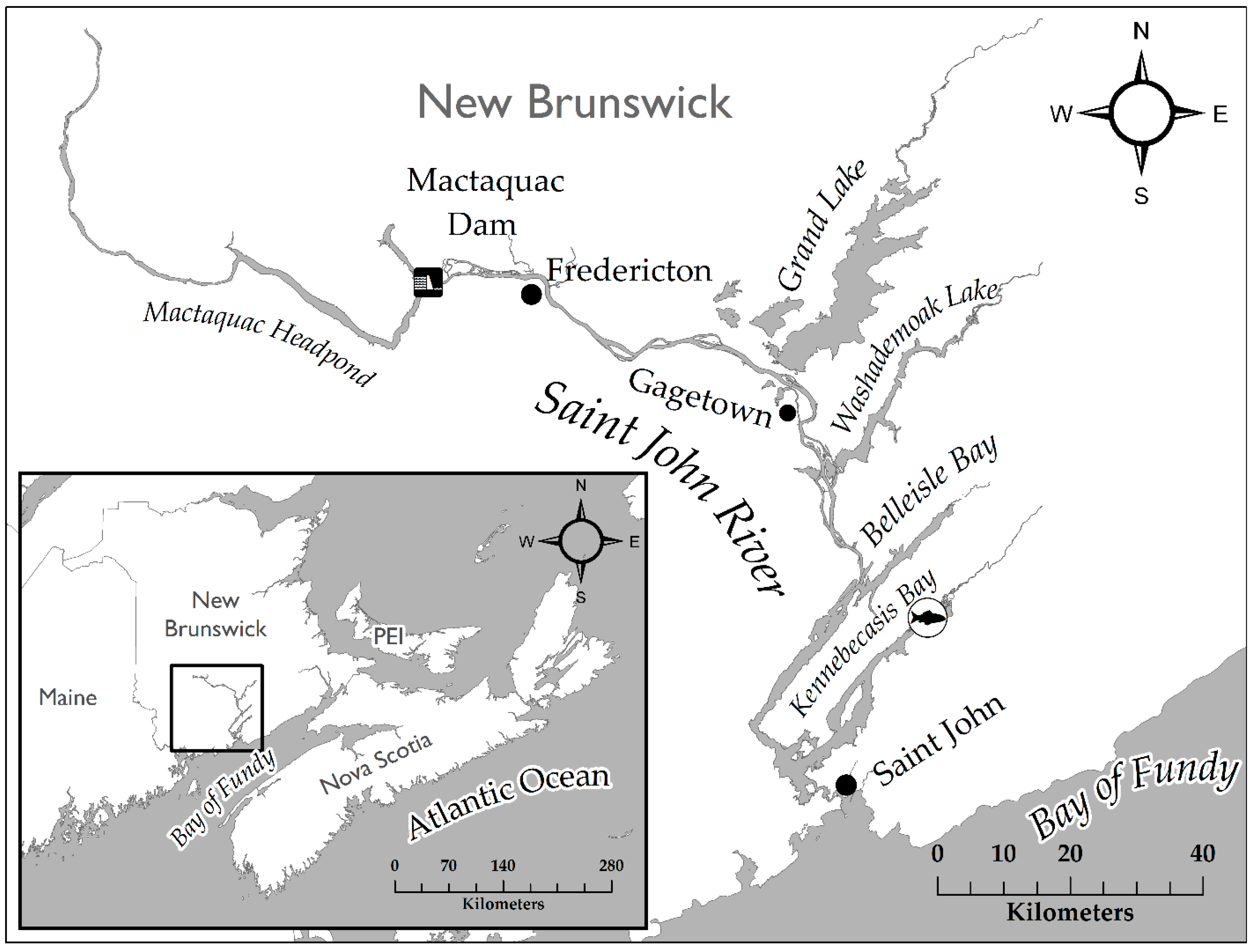
The SJR, New Brunswick (
Figure 1), is a large macro-tidal river draining into the western side of the Bay of Fundy at the City of Saint John. The river receives tidal influence to the City of Fredericton, ~130 km upstream from the river mouth and saltwater extends to the village of Gagetown [
29]. The SJR is fragmented by three large main-stem hydroelectric dams—of which, the Mactaquac Dam is the largest and most downstream barrier, limiting the movements of Shortnose Sturgeon to the lower 150 km of the river. The main stem of the SJR is fed by four major tributaries including Grand Lake, Washademoak Lake, Belleisle Bay and the Kennebecasis Bay, with sequentially increasing tidal fluctuations. The upstream end of the Kennebecasis Bay contains a well-documented winter aggregation of Shortnose Sturgeon [
9,
10], which annually occupies a sandy, 4.5–7 m deep location at the confluence of the Hammond and Kennebecasis Rivers. During winter, much of the river becomes ice bound except for the Reversing Falls, which merges to the Bay of Fundy through a dynamic cataract that remains ice-free year-round.
2.2. Workflow
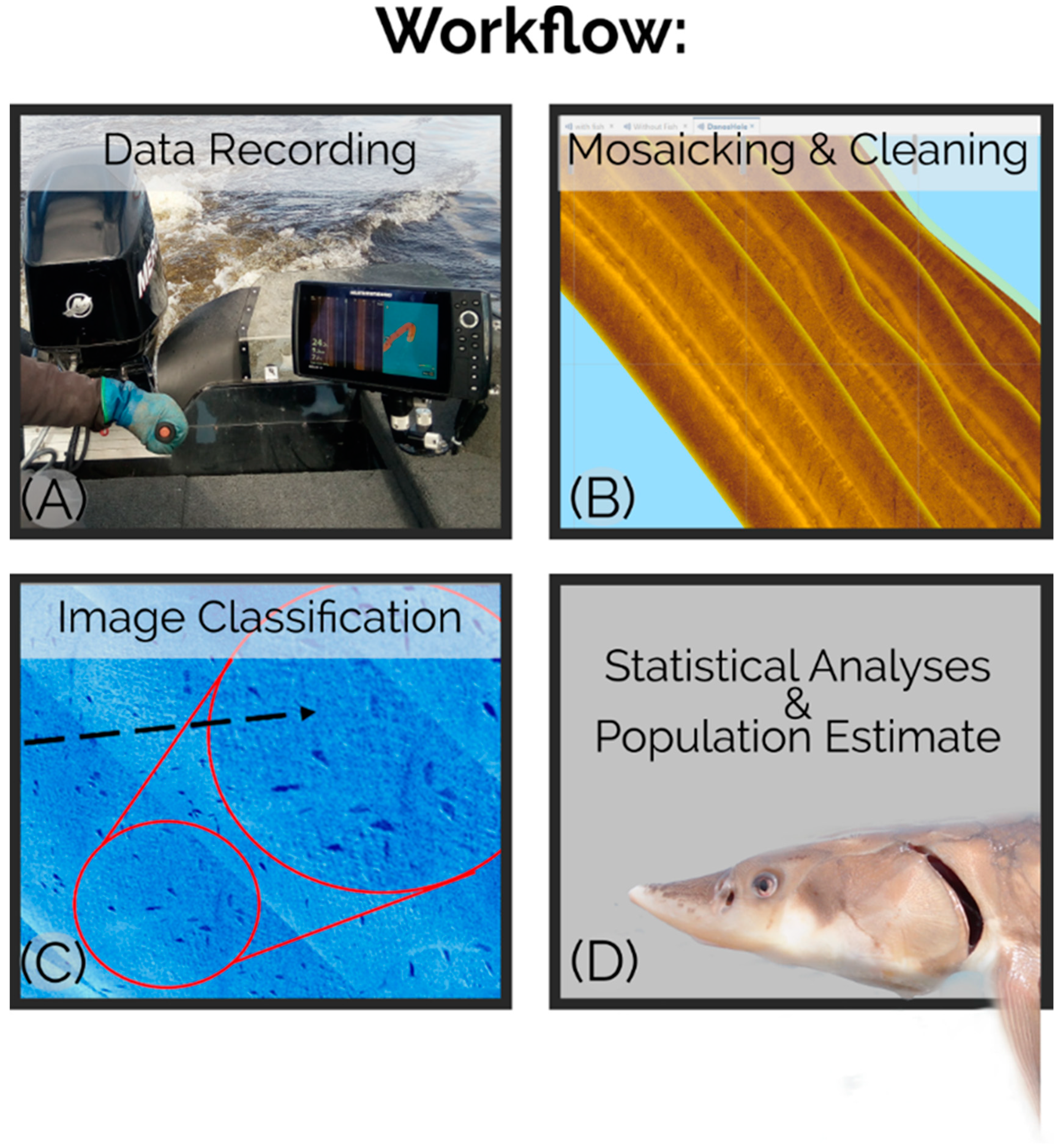
To produce our estimate of the SJR Shortnose Sturgeon population, river transects were driven over the major undescribed winter aggregation of Shortnose Sturgeon while continuously logging side-scan sonar data with a Humminbird (Johnson Outdoors, Racine, WI, United States) Helix 10 MEGA SI fish finder (
Figure 2). These data were aggregated in Reefmaster
® software (Reefmaster Software Ltd. Birdham, UK) to produce a mosaic image and exported as mtbtiles file for manipulation in GIS [
30]. Image pixels were then classified as “Sturgeon” or “river bed” in GIS to produce a population count in the surveyed region. The population count was then compared to four years of continuous Shortnose Sturgeon tracking data to produce a population estimate for the river and each identified winter aggregation therein.
2.3. Field Data Recording
Side-scan sonar surveys were conducted using a commercially available Humminbird® Helix 10 MEGA SI fish finder mounted to a Lund Rebel 1625XL fishing boat (Lund Boat Company, New York Mills, MN, United States) and sonar tracks were saved on a Humminbird® Zero Lines SD map card. Side-scan sonar tracks were recorded at a frequency of 1275 kHz (Humminbird MEGA imaging®) at a ping rate of 26.1 pings per second and a scanning range of 26 m to either side of the survey vessel. Survey speed varied from 7–10 km/h during transects and each survey was conducted as one continuous logged track. During surveys, the Humminbird® head unit with integrated GPS (Global Positioning System) was mounted 1 m to the port side of the side-scan transducer to provide an accurate reference to the actual position of individual Sturgeon detected by the side-scan transducer.
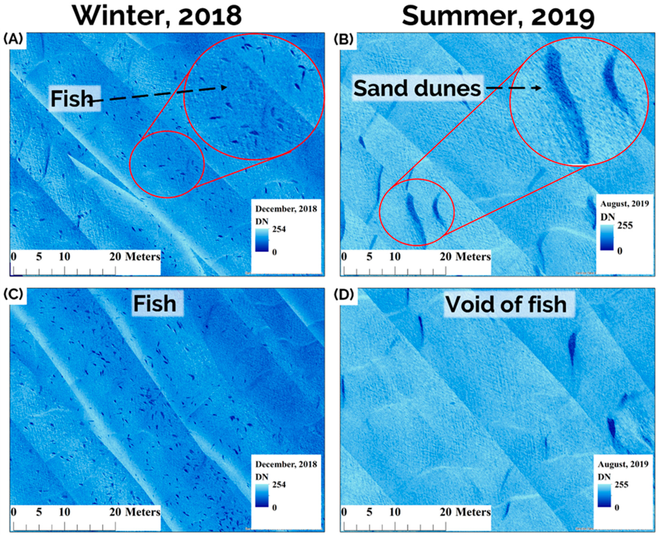
The primary winter survey was conducted on 11 December 2018 (winds < 6 knots, water temp = 0.6 °C) when our previous tracking data indicated that Sturgeon were densely aggregated in their winter habitats. Tagged Sturgeon were observed to arrive to the survey location as late as 22 December (acoustic tracking data collected in 2017) requiring comprehensive surveys to take place as late in the year as ice conditions permitted to provide the most comprehensive survey of the aggregation. A control summer survey was conducted on 24 August 2019 (winds < 5 knots, water temp = 23.4 °C) to corroborate with acoustic data that the area was indeed a winter habitat. We chose to complete each survey during a single outgoing tide as we observed that this is the time of least individual displacement based on sonar images. Sturgeon were commonly observed on sonar to move off bottom, re-position, and even rise to the surface during tide changes; behaviours that would all complicate clear image capture. These behaviours became less apparent as water temperature cooled in the late fall (see also [
9]), and our sonar imagery clearly showed all individuals to be positioned on the river bottom at the time of the survey described herein. We also selected calm weather days to conduct our surveys (i.e., winds < 6 knots) in order to minimize boat movement due to waves which facilitated driving straight equidistant transects and maximized image clarity. Total scan time for the winter and summer survey ranged between 6 and 4 h, respectively.
During surveys, transects were started upstream and to one side of the Sturgeon aggregation (so that Sturgeon were only visible on one side of the sonar screen) and transects were continued downstream until Sturgeon were no longer visualized on sonar. Sequential upstream and downstream passes were conducted in parallel across the school until Sturgeon were no longer seen on screen. The total mapped area consisted of 287,040 m2 in the winter at an average depth of 6.7 m (range = 3.6–9 m) and 254,800 m2 in the summer with an average depth of 5.7 m (2.6–7.9 m). Differences in depth were due to seasonal water level, slight variation in area covered, tidal level, and transect path.
2.4. Side-Scan Sonar Image Mosaicking and Filtering
Side-scan sonar produces photograph-like images of river bed texture [
31]. The transducer sends out a narrow, high-frequency acoustic beam perpendicular to either side of the boat and records the amplitude of the returning echo [
32]. The side scan produces multiple scanlines every second and simultaneously, the Humminbird
® fish finder records the GPS location approximately 1 to 3 times per second. When recorded on a moving boat, these scans provide a (near) continuous coverage of the riverbed [
31]. Using a post-processing software, the continuous vertical scanlines are stacked horizontally and compiled using the positional data, to produce a 2D acoustic image (i.e., echogram). Multiple options are currently available to combine side-scan data collected using consumer-grade fish finders [
33]. We used a commercially available, easy-to-use, closed-source software, Reefmaster
®, that creates maps from multiple different types of customer-grade fish finders [
30,
33]. The user-friendly settings available on Reefmaster
® allow the user to apply basic filters to clean the imagery before creating the mosaic.
The recorded tracks were uploaded into the Reefmaster
® software and corrected to a transducer depth (0.2 m) and distance from the internal GPS (1 m) [
30]. The tracks were combined to single mosaic images using “Bend Closest Display”. This setting prioritizes the signal closest to the center of the side-scan transect and blends the tracks close to the end of the swath when overlapping data exists [
30]. The input was then processed through 1x noise reduction and 100% autogain to equalize the brightness across the image. In order to ensure consistent side-scan tracks, the sections where the boat was moving too fast (>11.1 km/h) or turning too much (curve radius < 20 m) were removed from the image. These thresholds were found to be sufficient for keeping most of the data for analysis but removing possible high extremes resulting in image distortion. The sonar returns acquired closest to the survey vessel where some signal distortion was observed, and the far edges on the exterior of the swath, were removed from the image to maintain image quality. The removal of these areas resulted in some missing data in the mosaic where overlapping data did not exist. The default colour palette (RGB) was used, and the resulting images (both winter and summer) had a pixel resolution of 7.5 cm. Finally, the side-scan mosaic file was exported as a .mbtiles file.
2.5. Image Classification
Machine learning tools are almost ubiquitously applied to rapidly classify images, from fine [
34] to broad scales [
35]. These methods are also being used in fisheries, where researchers are combining sonar sensing methods and machine learning tools (e.g., [
36]). We used a well-established supervised maximum likelihood classification (sMLC) machine learning algorithm to classify the objects in the sonar images described above. sMLC is based on Bayesian probability theory [
37] and requires an initial training data suite to define the classes of interest. In this study, those classes were (1) potential Shortnose Sturgeon, and (2) river bed. These were manually delimited by visually identifying potential Shortnose Sturgeon, and the river bed in the sonar image,
n = 214 and
n = 11,207 pixels, respectively. Finally, we used these data to train the sMLC to classify the entire image as either potential Shortnose Sturgeon, or river bed. We conducted all data processing in ArcMap software (ESRI, Redlands, CA, United States [
38]).
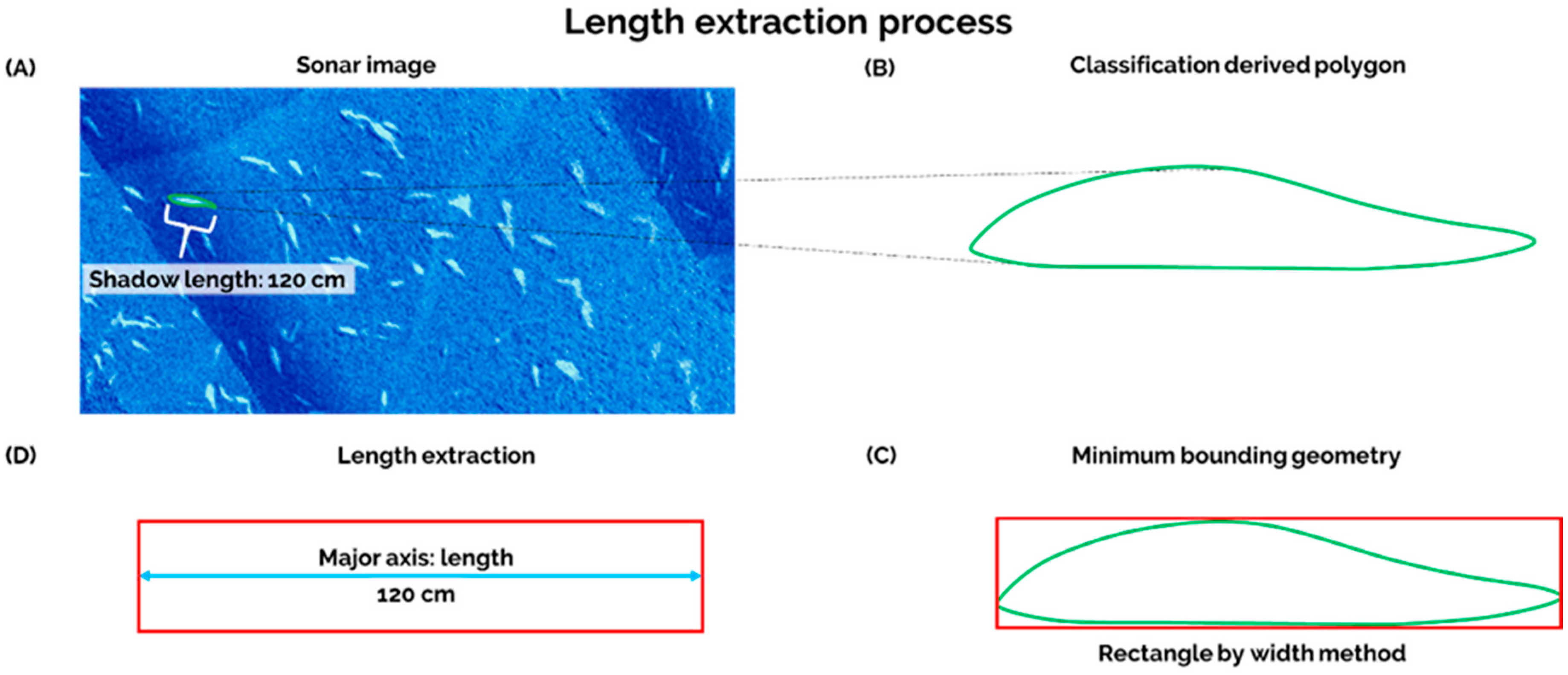
Upon completion of image classification, we applied a boundary condition to remove image noise, and potential detections that were outside the expected length range for Shortnose Sturgeon [
8]. These thresholds were set as: 20 cm < Potential Shortnose Sturgeon < 150 cm. To do so, we exploited the geometry of the derived image classification polygon. First, we ran a ‘minimum bounding geometry’ tool in ArcMap. The tool requires an initial input of points, lines, or polygons. First, the tool constructs a polygon around the input, and then geometry, i.e., length and width of the polygon, are derived by the tool. In this study, we use the classification polygons as the initial input. We selected the ‘rectangle by width’ option, which determines the longest distance of a classified polygon [
38] (
Figure 3A,B). The minimum bounding geometry tool calculates the length of the longest side of resulting rectangular polygon (
Figure 3C,D). Here, we assumed this was indicative of potential Shortnose Sturgeon length. Lastly, we implemented our boundary condition to obtain a count of potential Shortnose Sturgeon.
To test the validity of the sMLC to accurately classify the objects in the image, we carried out two analyses. The first analysis was a kappa coefficient (
k). This method is commonly used in image classification studies to examine the accuracy of the image classification against reference data, or ground-truthed data [
39].
k takes the form:
where
po = observed proportional agreement, and
pe = the expected agreement by change and,
while,
where
fi+ is the total for the
ith row, and
f+i is the total for the
ith column.
When
k > 0.8 this indicates a strong agreement between the reference data and the classified object; 0.4 <
k < 0.8 signifies moderate agreement, while
k < 0.4 is suggestive of poor agreement [
39].
A Chi Squared test (χ2) and was used to examine the number of potential Shortnose Sturgeon defined by the sMLC against those demarcated by the user. As there are no data available to compare modelled potential Shortnose Sturgeon with actual observations, we needed to manually inspect the image to identify what we considered potential Shortnose Sturgeon to run both analyses. We created a feature class in ArcMap using the ‘create feature tool’ and placed points on manually identified Sturgeon. Similarly, we conducted the same procedure for areas without fish, or river bed. We then used these points, and extracted values from our classified image, i.e., potential Shortnose Sturgeon or river bed. We used these data for both statistical tests (k and χ2), with a total of n = 65 manually selected Shortnose Sturgeon points, and n = 40 manually selected river bed points, ntotal = 105 for the winter image. All analyses were conducted in Excel 2016 (Microsoft corporation, Redmond, WA, United States).
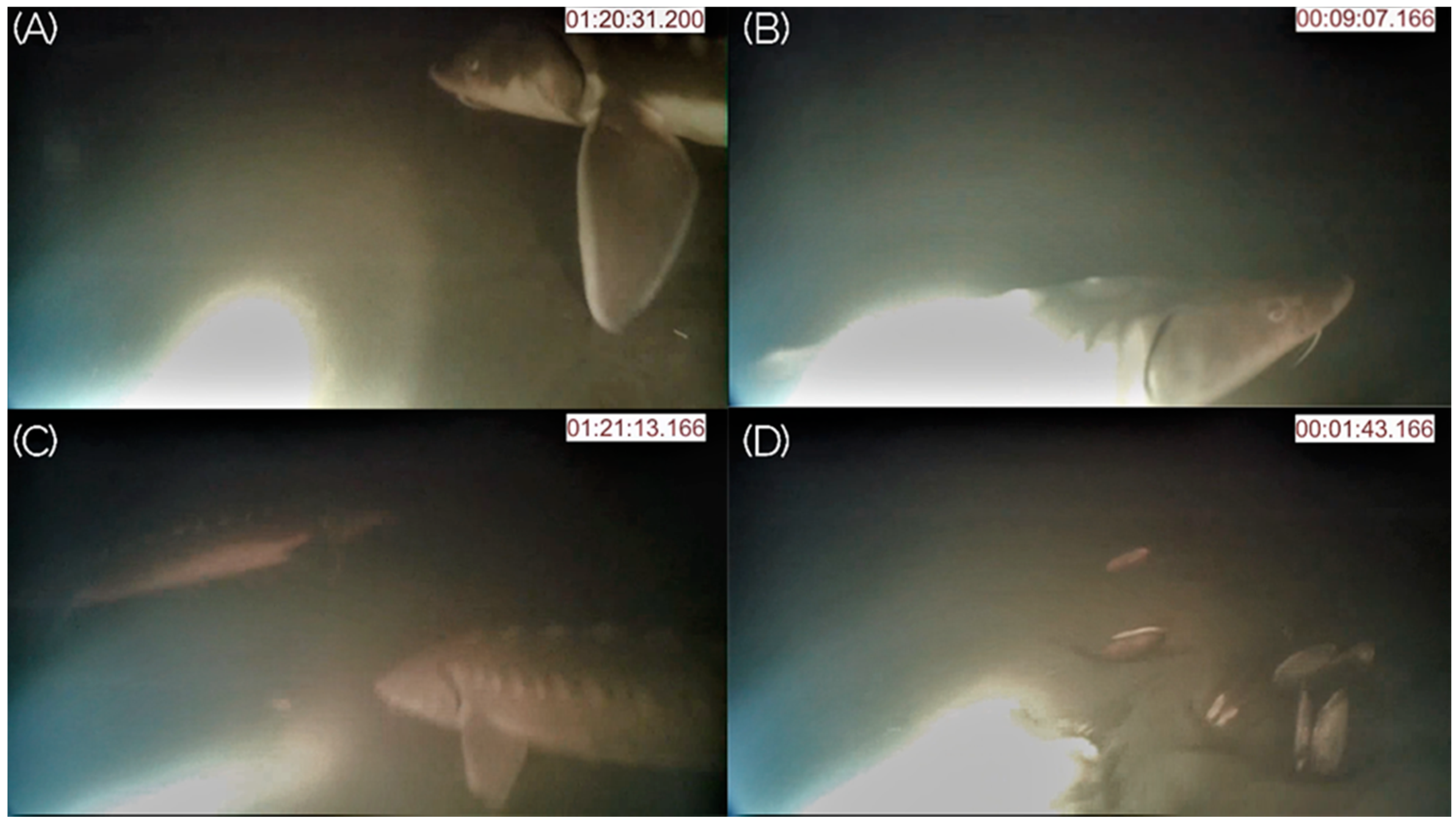
2.6. Underwater Camera Survey
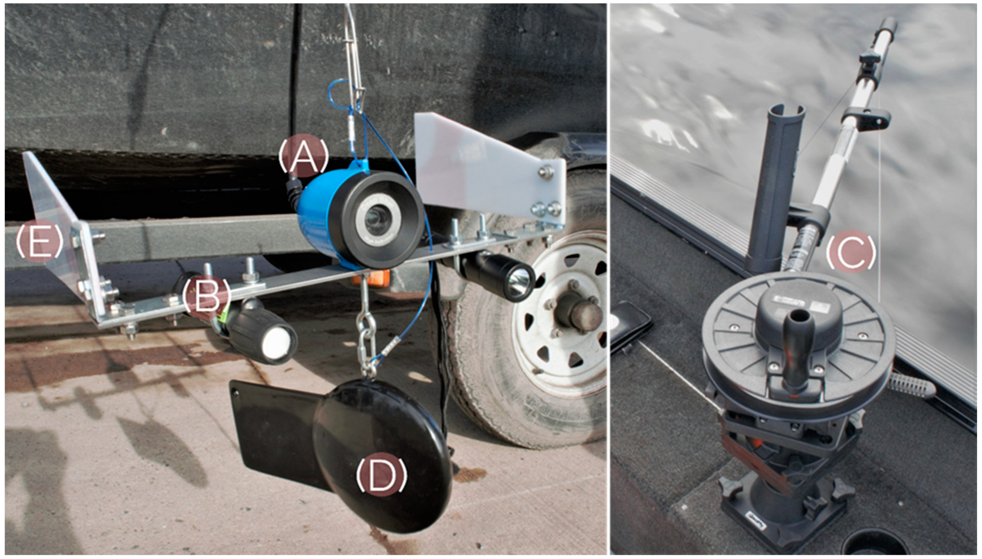
To further inspect the fish species and bottom structure in the study area, a video survey of the main aggregation was conducted on 27 November 2019. An underwater video camera (Deep Blue HDTVI, Ocean Systems Inc., Everett, WA, United States) was used for recording 30 frames/second High-Definition video as a .mp4 file to a memory stick (
Figure 4). Two scuba-diving flashlights were attached to facilitate filming close to the bottom in low light conditions (
Figure 4). The camera was set facing parallel to the bottom, and the maximum visibility was estimated to be 1–2 m. A 10 lb downrigger weight was used to lower the camera to the bottom (
Figure 4), and the depth of the camera was adjusted using a manual downrigger and live video feed so that the river bottom was continuously visible in the frame. The boat was maneuvered on idle (speeds between 1.1 km/h to 4.4 km/h) around the area for 109 min during which the boat covered a total distance of 2681 m.
The resulting video was analyzed, and all fish observed were counted. When possible, the fish species was identified. The bottom substrate was described, and all objects were recorded.
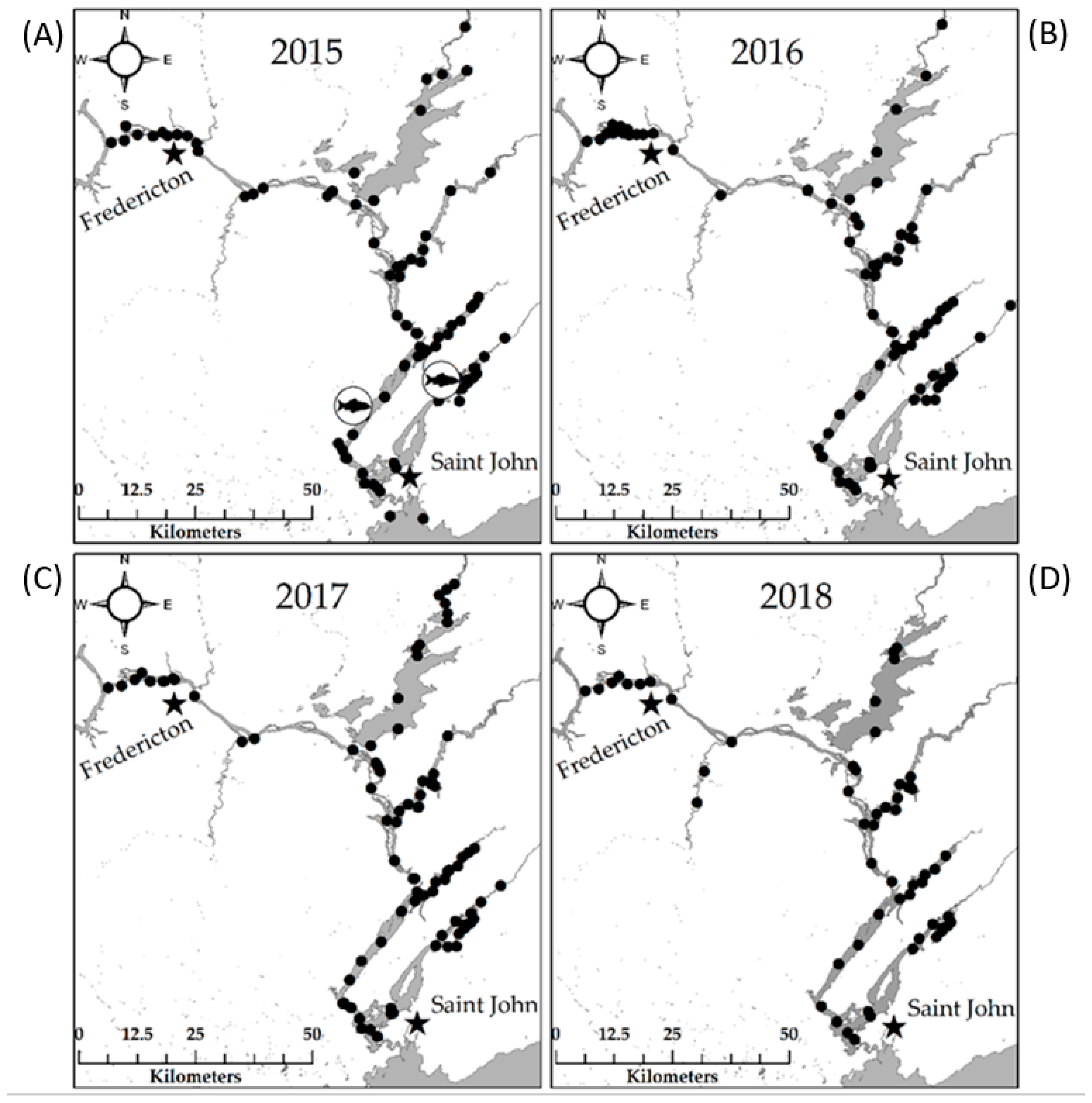
2.7. Tagging
Adult Shortnose Sturgeon (
n = 18; total length range= 100.5–128 cm, age estimate 25–43 years) were captured by gillnet in the SJR from 16–30 May 2015 (
n = 16 in Long Reach,
n = 2 in Kennebecasis Bay) and surgically implanted with Vemco (Bedford, Nova Scotia, Canada) model V16-4L acoustics tags (see [
40] for detailed methodology) using an anesthetic of 40 mg/L solution of 10 part ETOH: 1 parts clove oil. Tagged individuals were tracked by a project-specific array of Vemco VR2W receiver placements (
n = 125 in 2015,
n = 128 in 2016,
n = 135 in 2017, and
n = 60 in 2018) to identify winter habitats and the annual winter residency of tagged individuals therein (
Figure 5).
Following four years of continuous tracking, the proportions of tagged Shortnose Sturgeon occupying each of the five identified winter habitats annually were compiled. The mean proportional occupancy of tagged Sturgeon in the winter habitats located in this study was used to estimate the full SJR Shortnose Sturgeon population from the side-scan survey data. Following this calculation, the population of each winter habitat identified within the SJR was calculated from these same occupancy proportions as a mean percentage of the estimated total.
4. Discussion
Side-scan imaging using consumer-grade fish finders is becoming a popular tool for various ecological research applications such as fish habitat or mussel bed mapping [
13,
16,
20,
21,
22,
23]. Here we show that a consumer-grade side-scan sonar can be used to produce a mosaicked image of large-bodied fish, such as Sturgeon, close to the bottom. Further, we outline a rather simple classification method that can significantly reduce time in quantifying these types of data and remove user bias. The strong
k and χ
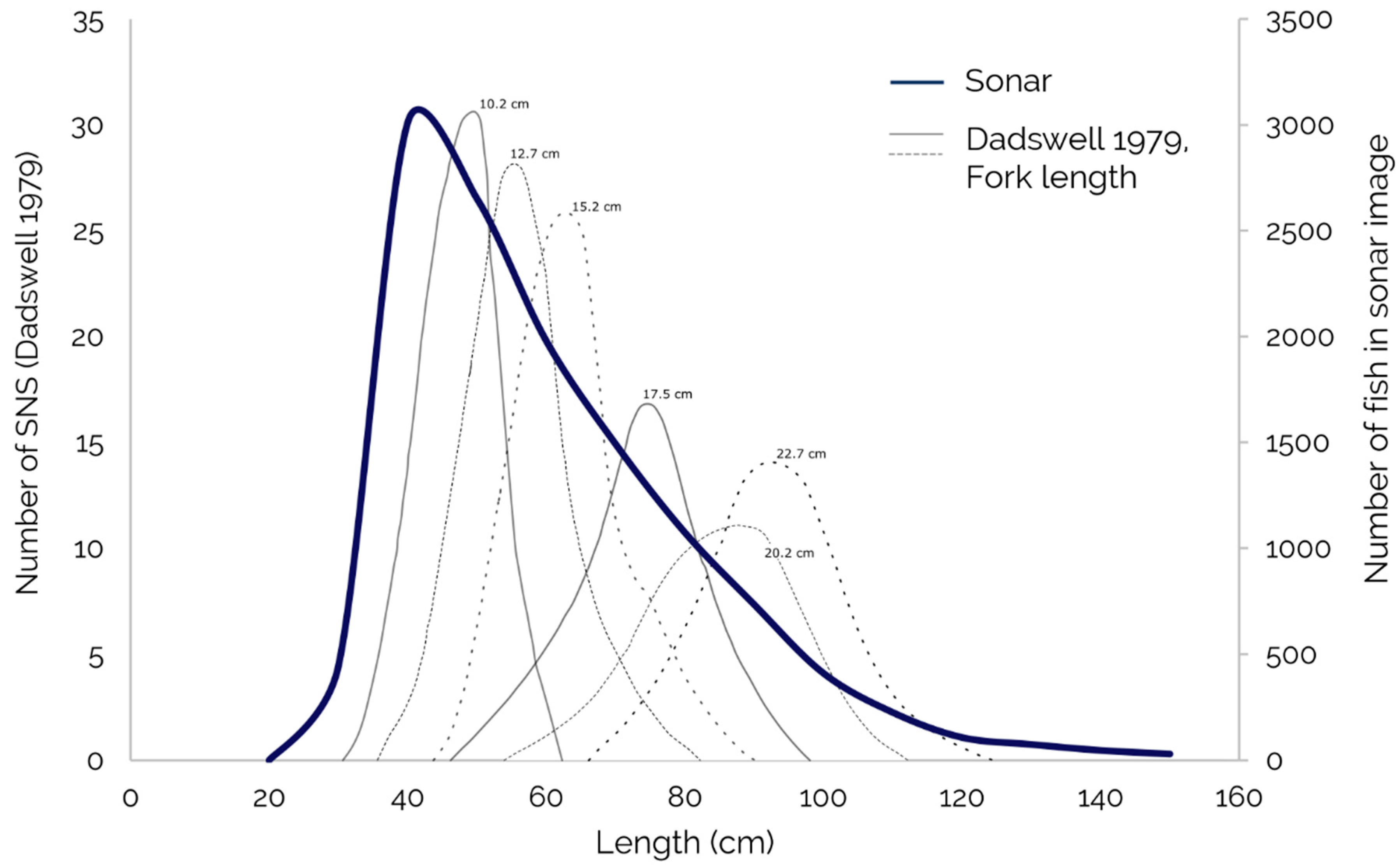
2 provide confidence in the efficacy of the sMLC as an adequate method to both classify and quantify Shortnose Sturgeon in our area of interest. Encouragingly, the frequency of distribution for Shortnose Sturgeon length provide a good fit to those obtained by a previous SJR gill net study in 1979 [
8] (
Figure 7). However, the frequency distribution curve in our data is skewed to the left of that from 1979 [
8]. This is likely a function of pixel resolution, where in our methods pixel resolution (7.5 cm) is too coarse to measure fork length as accurately as in the previous study [
8]. We suggest that with finer resolution sonar imagery, the methods applied in this study may facilitate the development of increasingly accurate estimates for size distributions across a large, aggregate fish population.
Sturgeon surveys employing side-scan sonar are not a novel approach (e.g., [
26,
27,
36]). However, these surveys have routinely been conducted during the summer months, which offers two distinct challenges for assessing population. First, Sturgeon are active during the warm water period either for the purpose of feeding or spawning making it difficult to obtain a robust accurate count of active individuals. Secondly, individuals can be widely dispersed over vast areas at these times rendering side-scan surveys impractical and unable to account for mixing and repeated observations. Conversely, winter surveys are ideal as species such as Shortnose Sturgeon aggregate densely during cold water periods [
2] and move little as water temperatures decline to winter minimum [
9] meaning that large aggregations can be captured by sonar in short periods of time and repeated counts (of the same individuals) are likely to be minimal. As an added benefit, Shortnose Sturgeon typically remain on the bottom during winter [
10] rather than occasionally swimming in the water column [
41] and are, therefore, more easily identified and even measured using sonar returns.
Although species identification is one of the most challenging tasks in hydroacoustic research [
42,
43], the observations from our underwater video surveys gives credence to our stipulation that the objects in the sonar image, and classified by sMLC, are mostly likely Shortnose Sturgeon. Shortnose Sturgeon were the only species identified in the underwater video survey and there were no other large objects observed in the video files. This was also confirmed by the size of the targets, the absence of other large fish tagged within the system (i.e., Atlantic Salmon;
Salmo salar, Striped Bass;
Morone saxatilis, Muskellunge;
Esox masquinongy, or Adult Atlantic Sturgeon;
Acipenser oxyrinchus that are also monitored within the SJR) and three years of exhaustive fall angling surveys which have exclusively captured Shortnose Sturgeon and exceeded 200 captured (and released) individuals. It is possible that juvenile Atlantic Sturgeon occupy the area in low numbers over winter which may inflate our estimates of the Shortnose Sturgeon population. However, no Atlantic Sturgeon were detected in our video survey or via angling, nor have they been documented in video surveys of other Shortnose Sturgeon winter locations in the SJR [
9,
10]. It is also of note that small Shortnose Sturgeon i.e., < ~40 cm FL were not apparent during video surveys, nor have they been captured in the location by angling. This may indicate that our method could visualize all fish of the size range present in our survey site, but also suggests that juvenile winter habitat likely occurs elsewhere in the SJR separate from the adults.
Using knowledge of Shortnose Sturgeon winter habitats acquired from acoustic tracking we were able to rapidly survey a high-density area to produce a population estimate for the entire SJR. Our whole river estimation of 20,101 is most likely an underestimate as data gaps were visible between sonar passes, resulting in missed fish. However, this estimate still aligns with that of a previous study [
8] that reported 18,000 ± 5400 individuals > 50 cm fork length. Furthermore, our population estimate for the Kennebecasis of ~2500 is similar to that produced and reported previously [
9,
10] for that region (3852–5222). While our estimate for the Kennebecasis is slightly lower than that produced by the aforementioned authors, we reiterate our acknowledgement that the numbers presented in this study likely underestimate the actual population size due to gaps in sonar coverage. We also note that the estimates produced and reported previously [
9,
10] are likely overestimates as they both assumed that Shortnose Sturgeon did not move at all during the winter and extended sampling period. Fish relocation within the Kennebecasis overwintering site likely resulted in repeated counts during the 2–3-month survey periods utilized previously [
9,
10] as opposed to estimates herein that were produced within hours.
Because the use of consumer-grade fish finders in research is rapidly growing, new fish finders and data analysis methods are constantly being developed. Standardization of data collection equipment, signal processing, and analyzation methods is needed to ensure quality and comparability in long-term monitoring. Despite our encouraging results, we must report on the limitations of the current method and in doing so propose methods that could mitigate or eliminate many of the assumptions and limitations of the first survey attempt described herein.
4.1. Sonar and Image Analysis Limitations
(1) Sonar transects were driven by hand and, therefore, were not of consistent speed, not perfectly straight, and often left gaps in sonar coverage. In the future, this type of survey would benefit from an autonomous drive routine to mitigate signal noise and data gaps.
(2) Movement of fish between the passing sonar tracks could result in duplicate counts or missed fish within estimates. This can be minimized by surveying the area as quickly as possible when water temperatures are at seasonal minimums during outgoing tides. Repeated, independent surveys within each overwintering site (e.g., three replicates in three consecutive days) would allow calculation of deviation between within-site estimates and thus, provide confidence limits.
(3) The minimum target detection of the side-scan sonar at the depths in which it was deployed and at the survey speed used remains unknown. Our frequency distribution of individuals > ~40 cm FL is similar to those reported in a 1979 tagging survey [
8]. However, it is unknown whether this detection length would extend below 40 cm FL. We suggest that side-scan technologies be tested with targets of known length at various depths to determine a minimum size of detection at different survey speeds and establish error values that could be applied to an automated length frequency calculation from sonar images.
(4) When Sturgeon are suspended off bottom, both the sonar return from the suspended Sturgeon and their resulting acoustic shadow are visible separately on sonar images. These suspended individuals may be double counted (counting both the fish and its shadow as unique targets) thus inflating estimates. This double counting can be most easily avoided by collecting sonar images during the period of greatest inactivity (outgoing tide during cold water periods) or through further training of the remote identification software.
4.2. Tracking and Population Estimate Limitations
(1) Winter habitat and whole river population estimates were calculated based on the winter locations of 18 telemetered individuals over four years. Despite the multi-year tracking and central tagging location, a larger sample size of tagged individuals representing a wider range of ages and sizes from throughout the river may more accurately reflect the distribution of Shortnose Sturgeon across winter habitats leading to more accurate estimates, and possibly finding of yet more overwintering locations.
(2) We conducted a side-scan sonar survey at only one, although major, overwintering location. The acoustic tracking data indicates minimally four other overwintering locations, and the best method to assess the population size at each other location is to repeat the side-scan survey at each of those locations rather than estimate population sizes based on proportion of the acoustically tagged population’s dispersal.
5. Future Questions
The simplicity of the survey method described here lends itself to produce rapid and repeatable surveys of large-bodied species, particularly Shortnose Sturgeon in the SJR during winter aggregation. Many of the limitations mentioned above can be addressed by repeated sampling, either between frequently collected temporal samples or through comparison of multiple years, as repeated datasets will facilitate assessment of the method’s accuracy. In addition, to improve the accuracy of our estimates, some questions remain to be answered:
(1) Do Shortnose Sturgeon and juvenile Atlantic Sturgeon intermix in winter habitats? We observed no Atlantic Sturgeon in the surveyed location during video surveys and did not capture them during extensive late season winter angling surveys. However, they may occur within the surveyed location sporadically at low densities.
(2) What conditions create favorable Shortnose Sturgeon winter habitat? In the future temperature, substrate, bathymetry, salinity, and current velocity should be monitored to accurately describe occupied habitats and individual distribution and orientation within those habitats.
(3) What is the measurement error associated with bottom target identification by side-scan sonar? Sonar targets can be measured, which allows the calculation of size distributions for targets. However, due to the shape of the side-scan sonar beam, an error is associated with the length of each identified target. Future research should aim to address this.
(4) What is the minimum size of target identification for the employed side-scan sonar? In the previous 1979 report [
8] the population of Sturgeon > 50 cm FL was estimated; however, we are unsure of the smallest fish that can be resolved in our sonar images. Small Sturgeon were not observed during video surveys or ever captured in angling surveys. Efforts should be made to determine the effective resolution minimums of the side-scan sonars used at a variety of scanning speeds.
6. Conclusions
The combined sonar and image classification method presented here provides a rapid and low-cost method for producing population estimates for Shortnose Sturgeon in an overwintering area and for monitoring river-wide population changes. The same method could be easily adopted in other areas for mapping other large fish or aquatic life.
Our estimate of >12,000 Shortnose Sturgeon occurring in a single large overwintering aggregation in the SJR and a greater estimate of >20,000 individuals >~40 cm FL within the entire SJR remains comparable to the mark recapture estimate produced in a previous study in 1979 [
8] (i.e., 18,000 ± 5400 > 50 cm FL). The 1979 estimate [
8], however, took five years to produce along with considerable effort and funding and, therefore, has limited repeatability, while our side-scan method was conducted in a few hours with inexpensive equipment available to the average recreational angler and without specific research funding. Furthermore, the clear identification of >12,000 Shortnose Sturgeon in the main aggregation alone, despite gaps in sonar data, nearly triples the current SJR population estimate even before considering our estimates for the four other winter aggregations.
From these preliminary surveys, it appears that the Shortnose Sturgeon population of the SJR, New Brunswick, has remained stable since first enumerated in 1979 [
8]. In fact, the true population may even be higher than previously thought, although it remains unknown whether or how the population may have been affected following the construction of the Beechwood Dam in 1955 and the Mactaquac Dam in 1968, collectively obstructing ~200 km of river habitat with undocumented habitat importance for the Shortnose Sturgeon population. As the SJR remains the sole spawning river for this species in Canada, we see no reason to remove the fisheries protections afforded to the Sturgeon population (i.e., mandatory catch and release angling) despite the indication of stable abundance. Current fisheries management appears to be effective in maintaining this unique population despite the construction of hydroelectric dams near suspected spawning locations [
5]. Those management policies and practices should, therefore, be continued for the protection of this unique species and possibly one the world’s few Sturgeon populations not facing precipitous decline.

 ,
, 


