Afromontane Forest Diversity and the Role of Grassland-Forest Transition in Tree Species Distribution


1
School of Biological Sciences, University of Canterbury, Private Bag 4800, Christchurch 8140, New Zealand
2
Department of Plant Science and Biotechnology, University of Jos, P.M.B. 2084, Jos 930001, Nigeria
3
Nigerian Montane Forest Project, Yelwa Village 663102, Taraba State, Nigeria
4
Ecology and Evolutionary Biology, University of Michigan, Ann Arbor, MI 48109, USA
5
Forest Global Earth Observatory, Smithsonian Tropical Research Institute, Washington, DC 20036, USA
*
Author to whom correspondence should be addressed.
Diversity 2020, 12(1), 30; https://0-doi-org.brum.beds.ac.uk/10.3390/d12010030
Submission received: 7 November 2019
/
Revised: 23 December 2019
/
Accepted: 7 January 2020
/
Published: 15 January 2020
(This article belongs to the Special Issue Biodiversity of Vegetation and Flora in Tropical Africa)
Abstract
:Local factors can play an important role in defining tree species distributions in species rich tropical forests. To what extent the same applies to relatively small, species poor West African montane forests is unknown. Here, forests survive in a grassland matrix and fire has played a key role in their spatial and temporal dynamics since the Miocene. To what extent these dynamics influence local species distributions, as compared with other environmental variables such as altitude and moisture remain unknown. Here, we use data from the 20.28 ha montane forest plot in Ngel Nyaki Forest Reserve, South-East Nigeria to explore these questions. The plot features a gradient from grassland to core forest, with significant edges. Within the plot, we determined tree stand structure and species diversity and identified all trees ≥1 cm in diameter. We recorded species guild (pioneer vs. shade tolerant), seed size, and dispersal mode. We analyzed and identified to what extent species showed a preference for forest edges/grasslands or core forest. Similarly, we looked for associations with elevation, distance to streams and forest versus grassland. We recorded 41,031 individuals belonging to 105 morphospecies in 87 genera and 47 families. Around 40% of all tree species, and 50% of the abundant species, showed a clear preference for either the edge/grassland habitat or the forest core. However, we found no obvious association between species guild, seed size or dispersal mode, and distance to edge, so what leads to this sorting remains unclear. Few species distributions were influenced by distance to streams or altitude.
1. Introduction
Afromontane forests are widespread across the African highlands [1,2,3]. Typically occurring above 1500 m in elevation, they extend from the Arabian Peninsula south along the rift to the Drakensberg Mountains in the east. In Western Africa, they are restricted to the Cameroon volcanic line and the Guinea highlands [1,4] (Figure 1). This disjunct distribution is ancient, pre-dating the Miocene doming that resulted in the Rift Valleys and the aridification of the East African interior [5]. Despite this distribution, Afromontane forests have a distinctive fauna and flora and harbor a high proportion of endemic species [6,7,8]. They have substantial carbon stocks [9], provide watershed protection [10] and other important ecosystem services [11]. However, Afromontane forests tend to occur in areas of high human population density and are under intense threat from agricultural practices, fire, and grazing [7,12]. Long-term monitoring of these forests is crucial for understanding how they function and for predicting their dynamics, essential information for sustainable management and preservation of the local and global services they provide.
Afromontane forests are characteristically small and fragmented; they typically occur within a grassland matrix and in West Africa the relative extent of grassland vs. forest has shifted in response to climate fluctuations since the Pleistocene [1,8,13]. Grasslands have dominated over the past 5000 years [14,15], and especially the last 3000 years [16]. Today, a combination of local climate and fire dynamics dictate the balance between grassland and forest [1,17,18,19], with the forest/grassland boundary reflecting the equilibrium between two processes. First, the progressive woody plant encroachment from the forest into the savannah/grassland, with propagules of woody species taking advantage of high-light conditions and lack of competition in the savannah [20,21]. Second, the elimination of woody plant seedlings, saplings and juveniles by grassland fires. Burning leads to a sharp boundary between forest and savannah/grassland [22,23], which is especially pronounced when fires are lit annually and used as a management tool for cattle grazing. In contrast, if fire is suppressed sufficiently, woody plants colonize the savannah/grassland forming narrow but distinct species-rich transition zones. Eventually, given sufficient time and protection from fire, the woody plant encroachment process continues and forests form [20,24]. Once established, the forest remains relatively self-protected from burning because of the lack of fine grass fuel required for intense/frequent fires, more shady conditions, and in general a different microclimate that makes it less prone to burn [25].
The historic dynamic equilibrium between forest and fire has major implications for forest structure and dynamics [8]. Having survived for thousands of years as islands of forest within a grassland matrix, Afromontane forests have long experienced strong edge effects. How these effects filter species and traits and thus impact forest composition is under investigation in the Afro-temperate forests of the Drakensberg Mountains of South Africa [1,26]. To what extent the South African situation applies in West Africa is currently unknown, although the fact that Le’zine, et al. [10] have recently confirmed extreme climate-related fluctuations in forest cover in the Cameroon highlands (the focus of this study) suggests a similar scenario. To begin to answer this question, we document tree species composition within a 20.28 ha permanent forest plot comprising mid-altitude montane forest and grassland, and explore correlations between tree species distributions and four environmental gradients: the proportion of grass surrounding individual trees (forest versus grassland), proximity to the grassy matrix/forest edge, elevation, and distance to streams (a proxy for soil moisture). In our study we tested the hypothesis that we would find a gradient in tree species composition and functional traits reflecting the core-edge gradient. We thought species sorting from the core to the edge should result from the progressive encroachment of forest into the grassland matrix via dispersal of small seeded, light tolerant species [26].
Finally, because West African montane forests are relatively understudied compared with those elsewhere in Africa, we compare our inventory statistics with those of other Afromontane forests.
2. Materials and Methods
2.1. Study Area and Study Site
The study was conducted in the 260 × 780 m (20.28 hectares) Ngel Nyaki Forest Dynamics Plot, part of the Smithsonian Forest Global Earth Observatory network (Forest-GEO). The plot coordinates are 07°04′05″ N in latitude and 11°03′24″ E in longitude, with an elevation range of 1588 m to 1690 m. The plot is within the 5.7 km2 Ngel Nyaki forest, located within the 46 km2 Ngel Nyaki Forest Reserve on the Mambilla Plateau, Taraba State [27,28] (Figure 1). The Nigerian Montane Forest Project (NMFP) [29] is based on the edge of the forest and collects regular weather data. The mean annual rainfall is 1800 mm, with most rain falling between April and October and a six-month dry season. The mean annual temperature is 19 °C and the monthly mean maximum and minimum temperatures for the wet and dry seasons are 25.6 and 15.4 °C, and 28.1 and 15.5 °C, respectively (NMFP weather data). The soil in Ngel Nyaki forest is volcanic and has a high clay content and a pH ranging between 6 and 6.5 [27]. Despite its relatively high nutrient content, the forest soil is easily leached.
Ngel Nyaki forest is floristically diverse and contains six International Union for the Conservation of Nature (IUCN) Red-Listed tree species including Entandophragma angolense (Meliaceae), Lovoa trichiliodes (Meliaceae), Eugenia gilgii (Myrtaceae), Dombeya ledermannii (Malvaceae), Prunus africana (Rosaceae), and Khaya grandifoliola (Meliaceae) [30]. It is a Birdlife International Important Bird Area with several species of large-gaped birds such as hornbills (Tockus alboterminatus) and turacos (Tauraco spp.). Primate species include the endangered Nigeria-Cameroon chimpanzee (Pan troglodytes ssp. ellioti), the putty-nosed monkey (Cercopithecus nictitans), and the tantalus monkey (Chlorocebus tantalus). Smaller mammals include civet cats (Civettictis civetta) and rodents such as the African giant pouched rat (Cricetomys spp.). While the forest is a State Forest Reserve and therefore protected from hunting and grazing, in practice there is very little protection. To what extent past human disturbance has influenced species distribution is unclear. Forest edges have been farmed on the lower slopes of the forest and cattle have damaged a substantial proportion of the reserve. Within the plot however, there is little evidence of disturbance other than past cattle incursions at the edge.
2.2. Census
The plot was established and measured following the standard protocol of the Smithsonian Center for Tropical Forest Science [32]. We measured, tagged and identified to morphospecies, every free-standing woody plant with diameter at breast height (dbh) ≥1 cm between January 2015 and January 2016. Stem diameter was recorded at 1.3 m above the ground, except when buttressed or swollen. Measurements were taken 50 cm above large buttresses and 2 cm below the lowest point of swellings. Trees were mapped with the highest possible precision in the field, typically at 0.1 m resolution within 5 × 5 m quadrats. Species identification was carried out mostly in the field and supplemented with DNA barcoding. Voucher specimens were collected for each morphospecies and at least one duplicate voucher is held at the NMFP herbarium. DNA barcode sequences of all morphospecies are deposited in the Barcode of Life Data System [33].
2.3. Environmental Variables and Gradients Evaluated
We calculated the location of each individual tree along three “gradients”; grassland edge to core forest, distance to water, and elevation. The elevation was based on detailed topographic maps obtained during the installation of the plot. We also mapped the two streams that run through the plot. Whether a tree was located in “forest vs. grass” was based on a geo-located Google Earth [34] image. The image comprised channels in the RGB space. An area was considered to be “grass” when the red content in a 1 × 1 m pixel in a jpg image was 37% or more. This 37% cutoff in the red channel resulted in a binary habitat map for the area with a very precise concordance with the grass vs. forest distinction on the ground (Figure 2). To avoid spurious results when calculating the minimum distance to grass from each individual tree, we removed isolated grass-looking pixels within the forested area. We forced all pixels with known presence of trees to be “forest” pixels, so all the trees were, by definition, at a distance >0 from the grass.
After defining the environment, we calculated four variables for each individual tree:
- (1)
- The proportion of grass in a 20 × 20 m area surrounding the individual tree. Rather than count the grass vs. forest pixels in a 20 m diameter circle around each tree, we used a 20 × 20 m square window around each tree because it was computationally more efficient than defining a circle around each tree. Within this square we counted the number of red (grass) vs. other 1 × 1 m pixels and from this calculated the proportion of “grass” vs. forest pixels. We used this metric to indicate whether a species was a forest or grassland species. Our 20 × 20 m squares overlapped and were not necessarily independent of each other.
- (2)
- The distance to the closest grass pixel. This was calculated from the coordinates of each individual and the grass vs. forest binary map. This metric indicates if a species prefers the forest core (=far from grass) or the forest edge or the grassland itself (=close to the grass).
- (3)
- The shortest distance to any of two streams in the plot.
- (4)
- The local elevation.
2.4. Species Guilds
Our five-guild classification is modified from Hawthorne [35,36]: (1) pioneer; (2) non-pioneer light demanding—needs shade to germinate and establish but larger individuals need light; (3) cryptic pioneer—needs light to germinate and establish but can survive for many years as adult in the understory; (4) shade-tolerant; and (5) grassland. For species not included in Hawthorne’s 1995 Ghanaian study [35], we identified species guild from information on the species in the JSTOR online plant database [37].
Our seed weight data came from data collected on fruit and seed traits as part of the Nigerian Montane Forest Project [29] ongoing research. Twenty seeds from fruits of at least five individual trees across the forest were weighed to the nearest g and the average seed weight taken. Dispersal modes were based on fruit and/or seed morphology, as described in [38]. Fleshy fruits were considered animal dispersed and hard seeds in pods, ballistically dispersed. Winged seeds are wind dispersed and very heavy, large seeds embedded in a thick husk, gravity dispersed. Growth form, i.e., tree, shrub or strangler, and position in canopy (emergent, canopy, or understory) was based on [27]. In addition, trees growing in the grassland with obvious adaptations to fire were classified as savannah trees.
2.5. Data Analyses
As part of the first assessment on species composition and diversity conducted in the Ngel Nyaki Forest Dynamics Plot, we calculated abundances, basal area and Fisher’s alpha diversity on a per hectare basis (i.e., within squares of 100 × 100 m, each a subset of the entire plot) for three diameter classes: ≥1 cm, ≥10 cm, and ≥30 cm. We used 13 table combinations of our plot for our calculations so that we had a total of 182 1-ha plots from which we calculated our per hectare diversity indices. We analyzed diversity at three taxonomic levels: species, genus, and family.
The four observed environmental preferences (% of surrounding grass, distance to grass, distance to stream, elevation) were compared with null expectations. The null expectations for each species were obtained after 999 constrained torus translations, an adaptation of the standard or unconstrained torus translation (see Appendix A for more details on standard (unconstrained) and constrained torus translations). During a standard torus translation, all individuals are translated together as a rigid cloud of points [39,40,41]. The spatial pattern of the species (the spatial aggregation) is respected, but the relationship with the habitat map (the grass vs. forest map, or the streams, or the elevation) is broken. All of our translations were constrained to only happen within the forest, never in the grass (Figure 3). We used the same constrained translations to assess significant associations with the grass, the streams and certain elevations. We developed constrained torus translations instead of unconstrained or standard torus translations across the entire plot because the latter predicted many individuals within the grass itself, just because a significant proportion of the Ngel Nyaki plot is covered in grass. This unrealistic expectation is a meaningless null hypothesis to test; if we did test it, it would result in all species being significantly far from the grass, even those with strong preferences for the forest edge.
After generating the null expectations, we evaluated the significance of the associations. If the observed x for the species was greater or lower than 95% of the expected (null) x, then the species was considered significantly associated to x. For example, if the observed median distance to grass of the individuals of a species was greater than 95% of the expected median distance after 999 torus translations, the species was deemed “significantly far from grass”, i.e., a forest core specialist. In contrast, if it was lower than 95% of the expected median distances, the species was deemed “significantly close to grass”. We followed the same approach with each of the other environmental variables considered. We used a Chi-Squared test to examine the relationship between species position on the gradient and seed size and dispersal mode. We grouped seeds into four size classes according to their weight: small (<0.6 g), medium (0.6–1.5 g), large (>1.5–3.0 g), and very large (>3.0 g). All the analyses were performed in R, version 3.3.3 [42] using customized functions or the CTFS R package [43].
3. Results
3.1. Diversity and Abundance
A total of 41,031 trees were recorded with an average density of 2062 individuals/ha. The number of individuals ≥10 cm dbh and ≥30 cm dbh were 6931 (352/ha) and 1686 (85/ha), respectively (Table 1). We recorded 105 species belonging to 47 families and 87 genera in the 20.28-ha plot. Rubiaceae, with nine species, was the most diverse family, followed by Euphobiaceae and Fabaceae with six species each, and Meliaceae with five species. Fisher’s alpha at the 1-ha scale was 12.42 for all stems, 12.03 for stems ≥10 cm, and 9.55 for the largest diameter class (≥30 cm dbh) (Table 1). The most abundant species was Garcinia smeathmannii, an understory tree of the Clusiaceae family with 11,960 individuals (607.63/ha), representing approximately 30% of individuals ≥1 cm dbh (Table 2). This was followed by Deinbollia pinnata (Sapindaceae) with 3077 individuals (158.68/ha) and Pleiocarpa pycnantha (Apocynaceae) with 2142 individuals (107.51/ha).
3.2. Basal Area
Tree total basal area was 553.49 (27.52 ± 8.64 m2/ha) of which 90% was contributed by large-diameter trees ≥30 cm dbh. The basal area was dominated by the family Fabaceae (96.67 m2), followed by Meliaceae, Olacaceae, Burseraceae, Moraceae, Sapotaceae, and Icacinaceae. Anthonotha noldeae had the highest basal area, followed by Strombosia schefleri, Carapa oreophila, Santiria trimera, Trichilia monadelpha, and Leptaulus zenkeri (Table 2). The complete species list with total number of individuals and total basal area (m2) for every species is found in Table S1.
3.3. Species Distribution and Preferences
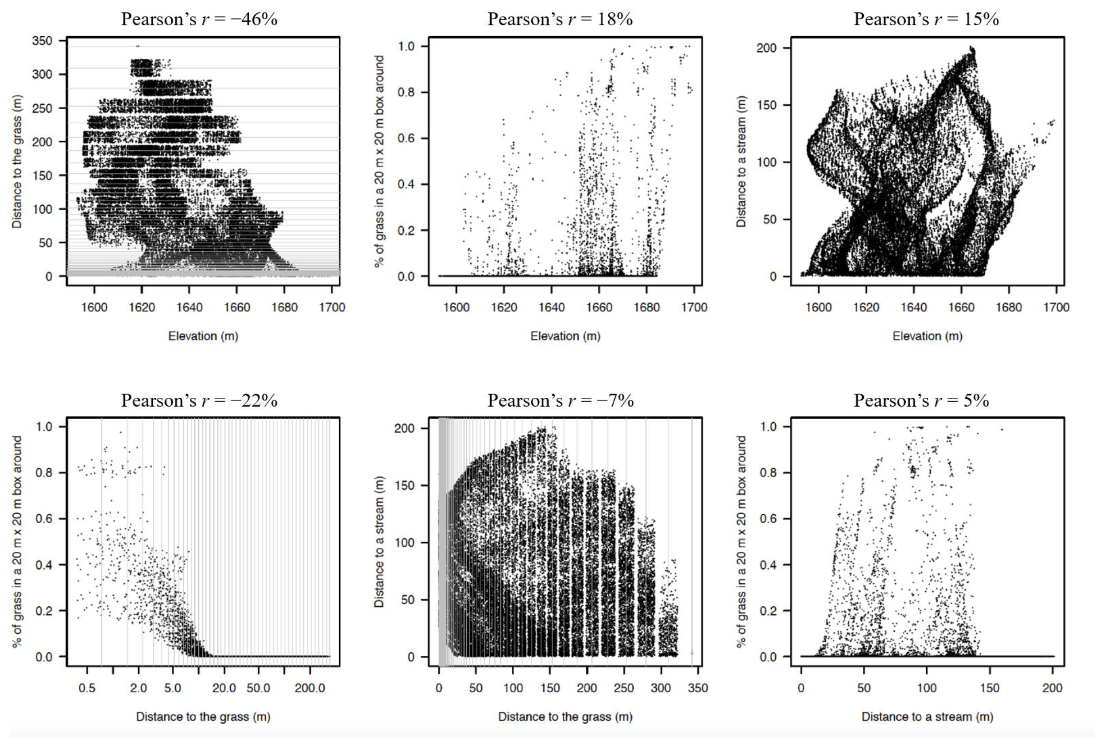
The four gradients (distance from edge, distance to stream, elevation, % grass) evaluated in the plot were weakly correlated with each other (Figure 4). Individual trees at higher elevations were closer to the grass (Pearson’s r = −0.46). The rest of the correlations were weaker than |r| = 0.30 (Figure 4).
The average individual values at the species level, however, showed stronger correlations, with some obvious elevational trends (Figure 5).
Many of the average preferences for the species did not differ from the expected by the random translations, suggesting that many of the species in Ngel Nyaki do not respond to the measured environmental gradients (See Table S2). The more common species however, showed stronger preferences (Table 3). All of the 65 abundant species (those with at least 20 individuals in the plot) were surrounded by significantly more or less grass than the expected by the null model. Four of these were clearly savannah species (Dombeya ledermannii, Entada abyssinica, Psorospermum aurantiacum, Rytigynia sp.) and two species (Clausena anisata and Guarea cedrata) mostly occurred in areas with a high percentage of grass (>50%) even though they are not savannah species. More than half of the common species (35) were significantly close (23) or far (12) from the grass. Around 20% of the common species (14) were significantly associated with high (8) or low (6) elevations. However, in contrast, few common species (6) were significantly close (5) or far (1, Chionanthus) from the stream.
Our analysis investigating the association between species position on the gradient and seed size or dispersal mode showed no relationship between position on the gradient and seed size (χ = 4.36, df = 6, p = 0.63) or dispersal mode (χ = 7.57, df = 6, p = 0.27). For example, species significantly closer to the grassland matrix ("edge” species in Table 3) had a median seed size of 0.25 g, twice the median size of those species significantly far from the grassland matrix (0.13 g; “core” species in Table 3). Twenty five percent and 75% quantiles for species close and far from the grass are 0.13–0.34 and 0.04–0.27 g respectively.
4. Discussion
Our study is the first detailed inventory of a West African montane forest that explores species distributions in relation to local environmental gradients. Our data are from the first census of the Ngel Nyaki Smithsonian Forest Global Earth Observatory plot.
4.1. Diversity and Composition of the Woody Plant Species
Within our total plant count of 41,031 trees with dbh ≥1 cm we recorded 105 species from 87 genera and 47 families. This is relatively low diversity compared with the results from previous studies in other tropical Afromontane forests. For example, Hamilton and Bensted-Smith [44], who recorded only trees with dbh >10 cm counted 104 species from the sub-montane forest of the East Usambara Mountains in East Africa. Dowsett-Lemaire, et al. [45], similarly including only larger sized trees recorded 232 species over 140 km2 in northern Malawi, with less diversity south of 14° S; e.g., 94 species in a forest of 11.3 km2 in Central Malawi. This drop in species diversity in Southern Malawi was due to range limits and several species ‘skipping’ southern Malawi and reappearing farther south [45]. However, in concordance with some Afromontane forests, e.g., forests in the Bonga region in East Africa [46], a high proportion (90%) of the genera at Ngel Nyaki were each represented by a single species and the most common families were Rubiaceae and Fabaceae [47,48].
Of the total woody plants encountered, 83% were small stems <10 cm dbh, as is typical in African [47,48,49] and non-African old-growth forests [50]. The African lowland forests of Korup (Cameroon), Ituri (Democratic Republic of the Congo), and Rabi (Gabon) contain even higher proportions of small diameter trees (92.3%, 94.8%, 93.6%, respectively). The same is observed in other tropical forests: BCI (Panama) (90.1%), Sinharaja (Sri Lanka) (91.8%), Lambir and Pasoh (both in Malaysia) (90.8% in each), and Yasuni, (Ecuador) (88.5%) [48,50].
The number of individuals of species in the plot varied considerably, from 11 singletons (e.g., Terminalia ivorensis and Olax sp.) to the extremely abundant Garcinia smeathmannii (Clusiaceae) with about 12,000 individuals (607 trees/ha). Garcinia smeathmannii, which makes up about one-third of the total tree abundance in the plot, is also the third most abundant species in the Rabi plot (Gabon), with 304 trees/ha [48]. Anthonotha noldeae (Fabaceae), an Afromontane endemic and one of the most common canopy species in Ngel Nyaki forest, showed the highest dominance if measured by basal area. This is of interest because locally, A. noldeae is only found in Ngel Nyaki forest and Cabbal Shirgu, and is absent from the rest of the Gotel mountains in Nigeria [51] and Mt Oku in neighbouring Cameroon [52]. We recorded 607 trees/ha of our most abundant species G. smeathmannii which is comparable to the abundance of 684 trees/ha of Dichostemma glaucescens in Rabi (Gabon) [48] and 535 trees/ha of Phyllobotryon spathulatum in Korup (Cameroon) [47]. About 39% of the species in the plot had <1 tree/ha, which when compared to other ForestGEO plots is similar to the 45% in Korup (Cameroon) and BCI (Panama), 34% in Pasoh (Malysia) and 40% in Yasuni (Equador), but lower than in the monodominant Ituri forest (Democratic Republic of Congo) where 72% of the species there are represented by <1 individual per hectare [47,50]. Among large diameter trees (≥10 cm dbh), Strombosia schefleri (Erythropalaceae) was the most abundant species with 35.3 trees/ha which is very similar to the abundance of Trichilia tuberculata (Meliaceae), the commonest large tree in BCI (Panama) with a reported abundance of 35 trees/ha. Although Ngel Nyaki is less species diverse when compared with many tropical forests of Africa, it comprised species both widespread across Africa and Afromontane endemics or near-endemics sensu White [2].
4.2. The Role of Environmental Variables
The main aim of this study was to look for evidence of local environmental factors influencing species distributions. In terms of core to edge gradients, we tested the hypothesis that species sorting from the core forest to the forest edge should result from the progressive encroachment of forest into the grassland matrix via dispersal of small seeded, light tolerant species [26]. We found partial support for this hypothesis in that 40% of all tree species and 50% of the abundant species did show a clear preference for either the edge/grassland habitat or the forest core. However, we found no association between position on the gradient and seed size or dispersal mode, which suggests that factors other than dispersal are influencing species distributions (see below).
Many of the species strongly associated with edge were expected; e.g., Entada abyssinica, Psorospermum aurantiacum, Rytiginia sp., and Dombeya ledermannii are all species restricted to grassland or the very edge of the forest, where light is always abundant. Other edge associated species such as Bridelia speciosa, Rauvolvia vomitoria, Millettia conraui, and Eugenia gilgii are also fire resistant, small to medium-sized pioneers, but occur in the understory as well as on the forest edge. Jackson [53] noted a similar guild in the Imatong Mountains of Sudan, and Adie, Kotze, and Lawes [26] in the Drakensberg montane forest of South Africa. That these light demanding species occur in the forest understory indicates their ‘cryptic pioneer’ [35,54] status. That is, they need light to germinate and establish but as they increase in size, they become more shade tolerant and can survive in the understory as adults for many years. Hawthorne [35] suggested that in Ugandan forests these shade tolerant traits may be adaptive and not necessarily present throughout a species range, which would be worth investigating. Of note is that in our study site the very common canopy legume tree, Anthonotha noldeae also fits the description of a cryptic pioneer. Anthonotha’s abundance on the forest edge and its likely nitrogen-fixing properties [55] suggests it is an important component of the forest flora, potentially playing a key role in forest expansion.
Species strongly associated with the core forest were all shade tolerant, forest species and included the emergent wind dispersed, Newtonia buchannii, and animal dispersed canopy species such as Drypetes gossweileri and Chrysophyllum albidum. Understory shade species included Voacanga africana and Dicranolepis grandifolia. Most of these core forest species are widespread across Africa and in Nigeria are a components of forests up to at least 1800 m in elevation [27].
Against our hypothesis for a core to edge gradient we found that almost 50% of species with ≥20 individuals in the plot (seven of which were in the 20 most abundant species in the plot), occurred throughout the forest, with no statistical preference for edge or core. Together, these species included almost the entire range of species guilds. For example, the understory tree species Carapa oreophila, Celtis gomphophylla, and Mallotus oppositifolius are ‘cryptic pioneers’, present deep within the forest as adults but showing no evidence of regeneration [56]. In contrast, species such as Parkia filicoidea, Entandrophragma angolense and Pouteria altissima are ‘Non-Pioneer Light Demanding’ [35] in that they need shade to germinate and establish, but as adults are light demanding. Shade tolerant understory species with no associations with either core or edge include Dasylepis racemosa, Diospyros monbuttensis, and Santiria trimera.
In contrast to our expectations, we found that species closer to the edge had, on average, larger seed sizes than the core species. So that unlike the situation in the South African temperate montane forests where small seeds are obviously key to forest success, we found that in West Africa, larger-seeded and fire-adapted species seem to dominate the edges of each forest patch. Other adaptations, like nitrogen-fixing nodules in Milletia [57] and likely A. noldeae [55] may help in seedling establishment and subsequent survival in the grassland matrix. In general, how these forest patches grow and function as species refugia during times of forest expansion [26] are exciting questions and opportunities for further research.
While the grassland to forest gradient was the steepest in our analysis, we also explored other potentially relevant gradients to further explain the distribution of tree species at Ngel Nyaki. For example, elevation gradients often play a key role in driving functional diversity [58]. We found 14 species were significantly associated with either low or high elevation within the plot. Among those associated with high elevation, Anthonotha noldeae, Clausena anisata, Entada abysinnica, Ritchea albersii, Rothmannia urcelliformis, and Tabanaemontana contorta were also associated with grass/forest edge and distance to grass, which makes sense considering that the grasslands are at high elevation in our plot.
Another gradient explored was distance to stream (a proxy for soil moisture) but this was only weakly associated to species distribution in Ngel Nyaki, with only 6 of our 65 abundant species showing significant associations to distance from stream ("wet” or “dry” species in Table 3). This was unexpected given that water availability is well known to play a key role in governing local patterns of plant distributions in many ecosystems [59]. For example, in the Barro Colorado Island plot, Comita and Engelbrecht [60] reported significant associations between species distributions and water availability. In contrast however, and more like us, Scalley, et al. [61] in the Luquillo wet montane forest plot in Puerto Rico found no association between the spatial distribution of tree species and stream locations, but rather, that stem density and species richness was highest in areas closest to streams.
Our findings may, to some extent, corroborate those of Adie, Kotze, and Lawes [26] who suggest that in the South African Drakensberg mountains, fire, coupled with harsh abiotic conditions have filtered Afrotemperate forest tree composition resulting in a prevalence of species traits such as small, bird-dispersed fruits and fire resistant bark across the forest. Such filtering could perhaps explain the presence of the long lived ‘cryptic’ pioneers Polyscias fulva and Trema orientalis throughout Ngel Nyaki forest. However, in Nigerian montane forests there is a range of species guilds and seed sizes; while some may reflect species filtering through the matrix, others are shade tolerant, late succession old forest species such as Santiria trimera [61]. Regarding S. trimera, both the stilt root and non-stilt root morphs occur at our study site. The separation between the morphs is deep rooted in the Santiria phylogenetic tree [62], therefore their presence at Ngel Nyaki perhaps suggests that Ngel Nyaki forest is ancient and was a forest refugia during periods of Pleistocene drying. Population genetic analysis following that of Koffi, Hardy, Doumenge, Cruaud and Heuertz [62] on Ngel Nyaki S. trimera and other forest tree species would help shed light on this. However, that Ngel Nyaki forest is the most species rich forest on the Mambilla Plateau [45] with several rare species [25] and some even new to science [63], and that A. noldeae occurs here in such abundance but almost nowhere else in West Africa, may again support the idea that Ngel Nyaki was a Pleistocene refuge. Moreover Brailsford [64] recorded high levels of chloroplast haplotype diversity at Ngel Nyaki as compared with other forest fragments on the Mambilla Plateau. Of course alternative explanations exist for the high diversity and again, molecular analyses would help shed light on this.
5. Conclusions
Our study provides the first detailed insight on patterns of species and trait guild composition in a West African montane forest. The Ngel Nyaki forest is similar to many other tropical and Afrotropical forests in terms of species diversity and dominance patterns. The gradient from forest edge to core is a key dimension of the niche as perceived by plants. Overall, ~40% of the individuals belong to species with significant preferences towards edges or forest core areas, which in turn represent ~45% of the local woody diversity. While dispersal abilities play a role in forest expansion, our data did not show any association between species position on the gradient and dispersal mode. Further research is needed to disentangle the effect of changes in forest patch size and environmental preferences of the species to make more accurate predictions of how Afromontane forests will behave under changing fire regimes and human disturbance in the region.
Supplementary Materials
The following are available online at https://0-www-mdpi-com.brum.beds.ac.uk/1424-2818/12/1/30/s1, Table S1, Total number of individuals and total basal area (m2) for each of the 105 species of trees with dbh ≥1cm recorded in the Ngel Nyaki 20.28-ha plot. Table S2, Associations between the distribution of the all species and four environmental gradients in Ngel Nyaki plot (Nigeria). Full census data are available upon reasonable request from the ForestGEO data portal, http://ctfs.si.edu/datarequest/.
Author Contributions
Conceptualization, I.A., G.A., D.K., and H.C.; data curation, I.A., D.K., and H.C.; formal analysis, I.A. and G.A.; funding acquisition, H.C.; investigation, I.A., G.A., D.K., and H.C.; methodology, I.A., G.A., D.K., and H.C.; project administration, H.C.; software, G.A.; supervision, D.K. and H.C.; visualization, G.A.; writing—original draft, I.A.; writing—review and editing, I.A., G.A., D.K., and H.C. All authors have read and agreed to the published version of the manuscript.
Funding
The setting up and enumeration of the ForestGEO plot in Ngel Nyaki, Nigeria was majorly funded by a donation from Retired General T.Y. Danjuma to the Nigerian Montane Forest Project and other smaller donations from Forest Global Earth Observatory (ForestGEO) of the Smithsonian Tropical Research Institute, Chester Zoo, England and the A.G. Leventis Foundation.
Acknowledgments
This study was made possible by the generous donation made by Retired General T.Y. Danjuma to the Nigerian Montane Forest Project (NMFP) through H. Chapman. We also thank Forest Global Earth Observatory (ForestGEO) of the Smithsonian Tropical Research Institute for the support towards the plot census. We also wish to thank Chester Zoo, England, and A.G. Leventis Foundation for their financial assistance to the NMFP. I. Abiem also received a PhD scholarship from the University of Jos, Nigeria. We wish to thank the staff of NMFP especially the ForestGEO team who carried out the tree census. We also wish to thank S. Russo for her enlightening suggestions on the scope and direction of this research and for her extremely generous mentorship to IA during the ForestGEO workshops. The idea for this manuscript was put together at the 2017 ForestGEO workshop supported by the US National Science Foundation (NSF) grant to S. J. Davies. GA was supported while conducting this research as part of the Next Generation Ecosystem Experiments-Tropics, funded by the U.S. Department of Energy, Office of Science, Office of Biological and Environmental Research.
Conflicts of Interest
The authors declare no conflict of interest.
Appendix A
Appendix A.1. Torus Translations
The goal of a torus translation is to break the relationship between a cloud of points (e.g., the individuals of a given species) and the space and consequently, any biotic/abiotic gradient that happens in the space.
Torus translation tests are routinely used in analysis of plant-habitat associations [40,41,42]. The rationale underlying torus translation tests is to contrast the observations with the expectations under the assumption of lack of relationship between a given species and the habitat. The expectation is generated by breaking the spatial relationship between the habitat map and the tree map.
While a simple approach to break the relationship between, e.g., trees and the space they occupy would be to randomize the location of each tree independently, this would treat each tree as an independent observation, which is incorrect. To avoid this problem, a torus translation is a translation of the entire cloud of points (the entire map of trees). In particular, it is a translation in a torus: when making a random “jump”, things that “disappear” by the right appear by the left, things that “disappear” by the north appear by the south, and so on.
Appendix A.2. Translating the Map vs. the Individuals
Previous implementations of the method, at least in large Forest GEO plots similar to Ngel-Nyaki, have translated a categorical habitat map in the torus. By doing so: (1) the relationship between individual trees and habitat is broken, and (2) the spatial aggregation of the individual trees is respected. Consequently, one can test whether a given species has more/less individuals within a given habitat than expected.
Exactly the same can be done by translating the trees themselves (i.e., translating the cloud of points that represent the individual trees. The result is the same: a relative translation between the map and the trees. Here, we decided to translate the points, not the map. We considered it more intuitive to think of variables like “distance to the stream”, “% of grass surrounding”, etc., as individual-level properties, more than variables in a map.
Appendix A.3. Constrained Translations
The point of making the torus translations is to generate a null expectation. Something with which to contrast the observations. The translations define a null hypothesis, and the null hypothesis must make sense. In our case, we were particularly interested in the forest vs. grass distinction. We wanted to know whether some species were closer to the grass than others (i.e., closer to the edge of the forest). The Ngel Nyaki plot itself, however, is not completely covered by forest. It has a substantial amount of grass within it. If we translated points to forest or grass indistinctly, we would end with many trees within the grass. This would generate the (erroneous) expectation of all the species being strongly associated with grass. By comparing that expectation with the observations, we would conclude that all the species are significantly far from the grass. Even edge specialists.
To avoid that we run constrained translations in the torus. Like standard torus translations, a constrained translation makes the trees jump together (as a rigid cloud of points) randomly in the torus. Unlike the standard torus translations, we added the constraint of never arriving in grass. Jumps were forced to be sufficiently long that they always arrived in forest rather than grass, while at the same time respecting as much as possible the relative position of the translated points. One way of thinking about this is as a non-perfect torus, narrower in places with more grass, and wider in places with more forest. The torus is still a torus, topologically speaking. Another way to think about this is to imagine a map with invaginations in the forbidden areas, on top of which a regular grid of coordinates is placed (with no invaginations), to serve as a reference for the translations.
In summary, a constrained torus translation is a translation of a cloud of points that respects, as much as possible, the relative position of the individuals. Species that are strongly aggregated have expectations composed of tight clouds of points, and vice versa. We inspected visually many translations and we concluded that the result was satisfactory for our purposes.
References
- Linder, H.P. The evolution of African plant diversity. Front. Ecol. Evol. 2014, 2, 38. [Google Scholar] [CrossRef] [Green Version]
- White, F. The Vegetation of Africa, a Descriptive Memoir to Accompany the UNESCO/AETFAT/UNSO Vegetation Map of Africa; UNESCO: Paris, France, 1983; 356p. [Google Scholar]
- White, F. The afromontane region. In Biogeography and Ecology of Southern Africa; Springer: Berlin/Heidelberg, Germany, 1978; pp. 463–513. [Google Scholar]
- Gehrke, B.; Linder, H.P. Species richness, endemism and species composition in the tropical Afroalpine flora. Alp. Bot. 2014, 124, 165–177. [Google Scholar] [CrossRef]
- Linder, H.P.; Lovett, J.; Mutke, J.M.; Barthlott, W.; Jürgens, N.; Rebelo, T.; Küper, W. A numerical re-evaluation of the sub-Saharan phytochoria of mainland Africa. Biol. Skr. 2005, 55, 229–252. [Google Scholar]
- Burgess, N.D.; Balmford, A.; Cordeiro, N.J.; Fjeldsa, J.; Küper, W.; Rahbek, C.; Sanderson, E.W.; Scharlemann, J.P.; Sommer, J.H.; Williams, P.H. Correlations among species distributions, human density and human infrastructure across the high biodiversity tropical mountains of Africa. J. Biol. Conserv. 2007, 134, 164–177. [Google Scholar] [CrossRef]
- Cordeiro, N.J.; Burgess, N.D.; Dovie, D.B.; Kaplin, B.A.; Plumptre, A.J.; Marrs, R. Conservation in areas of high population density in sub-Saharan Africa. Biol. Conserv. 2007, 134, 155–163. [Google Scholar] [CrossRef]
- Meadows, M.; Linder, H. Special Paper: A Palaeoecological perspective on the origin of afromontane grasslands. J. Biogeogr. 1993, 20, 345–355. [Google Scholar] [CrossRef]
- Spracklen, D.; Righelato, R. Tropical montane forests are a larger than expected global carbon store. Biogeosciences 2014, 11, 2741–2754. [Google Scholar] [CrossRef] [Green Version]
- Schröter, D.; Cramer, W.; Leemans, R.; Prentice, I.C.; Araújo, M.B.; Arnell, N.W.; Bondeau, A.; Bugmann, H.; Carter, T.R.; Gracia, C.A. Ecosystem service supply and vulnerability to global change in Europe. Science 2005, 310, 1333–1337. [Google Scholar] [CrossRef] [Green Version]
- Nadkarni, N.M.; Wheelwright, N.T. Monteverde: Ecology and Conservation of a Tropical Cloud Forest; Oxford University Press: Oxford, UK, 2000. [Google Scholar]
- Chapman, H.M.; Olson, S.M.; Trumm, D. An assessment of changes in the montane forests of Taraba State, Nigeria, over the past 30 years. Oryx 2004, 38, 282–290. [Google Scholar] [CrossRef] [Green Version]
- Lézine, A.-M.; Izumi, K.; Kageyama, M.; Achoundong, G. A 90,000-year record of Afromontane forest responses to climate change. Science 2019, 363, 177–181. [Google Scholar] [CrossRef]
- Lawes, M.J. The Distribution of the Samango Monkey (Cercopithecus mitis erythrarchus Peters, 1852 and Cercopithecus mitis labiatus I. Geoffroy, 1843) and Forest History in Southern Africa. J. Biogeogr. 1990, 17, 669–680. [Google Scholar] [CrossRef]
- White, G.C.; Burnham, K.P.; Anderson, D.R. Advanced features of Program Mark. In Wildlife, Land, and People: Priorities for the 21st Century; Field, R., Warren, R.J., Okarma, H., Sievert, P.R., Eds.; The Wildlife Society: Bethesda, MD, USA, 2001. [Google Scholar]
- Lézine, A.-M.; Assi-Kaudjhis, C.; Roche, E.; Vincens, A.; Achoundong, G. Towards an understanding of West African montane forest response to climate change. J. Biogeogr. 2013, 40, 183–196. [Google Scholar] [CrossRef]
- Eeley, H.A.; Lawes, M.J.; Piper, S. The influence of climate change on the distribution of indigenous forest in KwaZulu-Natal, South Africa. J. Biogeogr. 1999, 26, 595–617. [Google Scholar] [CrossRef]
- Dowsett-Lemaire, F.; Dowsett, R.J.; Dyer, M. Important Bird Areas in Africa and Associated Islands; Pisces Publications and BirdLife International: Cambridge, UK, 2001. [Google Scholar]
- Lebamba. Forest-savannah dynamics on the Adamawa plateau (Central Cameroon) during the “African humid period” termination: A new high-resolution pollen record from Lake Tizong. Rev. Palaeobot. Palynol. 2016, 235. [Google Scholar] [CrossRef]
- Venter, Z.S.; Cramer, M.D.; Hawkins, H.J. Drivers of woody plant encroachment over Africa. Nat. Commun. 2018, 9, 2272. [Google Scholar] [CrossRef]
- Müller, S.C.; Overbeck, G.E.; Pfadenhauer, J.; Pillar, V.D. Woody species patterns at forest–grassland boundaries in southern Brazil. Flora Morphol. Distrib. Funct. Ecol. Plants 2012, 207, 586–598. [Google Scholar] [CrossRef]
- Gignoux, J.; Konaté, S.; Lahoreau, G.; Le Roux, X.; Simioni, G. Allocation strategies of savanna and forest tree seedlings in response to fire and shading: Outcomes of a field experiment. Sci. Rep. 2016, 6, 38838. [Google Scholar] [CrossRef] [Green Version]
- Kotze, D.J.; Lawes, M.J. Viability of ecological processes in small Afromontane forest patches in South Africa. J. Austral Ecol. 2007, 32, 294–304. [Google Scholar] [CrossRef]
- Andela, N.; Morton, D.; Giglio, L.; Chen, Y.; Van Der Werf, G.; Kasibhatla, P.; DeFries, R.; Collatz, G.; Hantson, S.; Kloster, S. A human-driven decline in global burned area. Science 2017, 356, 1356–1362. [Google Scholar] [CrossRef] [Green Version]
- Van Langevelde, F.; Van De Vijver, C.A.; Kumar, L.; Van De Koppel, J.; De Ridder, N.; Van Andel, J.; Skidmore, A.K.; Hearne, J.W.; Stroosnijder, L.; Bond, W.J. Effects of fire and herbivory on the stability of savanna ecosystems. Ecology 2003, 84, 337–350. [Google Scholar] [CrossRef] [Green Version]
- Adie, H.; Kotze, D.J.; Lawes, M.J. Small fire refugia in the grassy matrix and the persistence of Afrotemperate forest in the Drakensberg Mountains. Sci. Rep. 2017, 7, 6549. [Google Scholar] [CrossRef] [PubMed] [Green Version]
- Chapman, J.; Chapman, H. The Forests of Taraba and Adamawa States, Nigeria an Ecological Account and Plant Species Checklist; University of Canterbury: Christchurch, New Zealand, 2001; p. 221. [Google Scholar]
- Beck, J.; Chapman, H. A population estimate of the endangered chimpanzee Pan troglodytes vellerosus in a Nigerian montane forest: Implications for conservation. Oryx 2008, 42, 448. [Google Scholar] [CrossRef] [Green Version]
- Nigerian Montane Forest Project. Available online: https://www.canterbury.ac.nz/afromontane/ (accessed on 6 November 2019).
- Borokini, T. A Systematic Compilation of IUCN Red-listed Threatened Plant Species in Nigeria. Int. J. Environ. Sci. 2014, 3, 104–133. [Google Scholar]
- Thia, J.A. The Plight of Trees in Disturbed Forest: Conservation of Montane Trees, Nigeria. Master’s Thesis, University of Canterbury, Christchurch, New Zealand, 2014. [Google Scholar]
- Condit, R. Tropical Forest Census Plots: Methods and Results from Barro Colorado Island, Panama and A Comparison with Other Plots; Springer Science & Business Media: Berlin, Germany, 1998. [Google Scholar]
- Barcode of Life Data System. Available online: https://www.boldsystems.org/ (accessed on 6 November 2019).
- The World’s Most Detailed Globe. Available online: https://www.google.com/earth/ (accessed on 6 November 2019).
- Hawthorne, W. Ecological profiles of Ghanaian forest trees. In Tropical Forestry Papers; Oxford Forestry Institute: Oxford, UK, 1995; Volume 29, pp. 1–345. [Google Scholar]
- Hawthorne, W.D. Holes and the sums of parts in Ghanaian forest: Regeneration, scale and sustainable use. Proc. R. Soc. Edinb. Sect. B Biol. Sci. 1996, 104, 75–176. [Google Scholar] [CrossRef]
- Global Plants. Available online: https://0-plants-jstor-org.brum.beds.ac.uk/ (accessed on 6 November 2019).
- Barnes, A.D.; Chapman, H.M. Dispersal traits determine passive restoration trajectory of a Nigerian montane forest. Acta Oecol. 2014, 56, 32–40. [Google Scholar] [CrossRef]
- Harms, K.E.; Condit, R.; Hubbell, S.P.; Foster, R.B. Habitat associations of trees and shrubs in a 50-ha Neotropical forest plot. J. Ecol. 2001, 89, 947–959. [Google Scholar] [CrossRef]
- Wiegand, T.; Moloney, K.A. Handbook of Spatial Point-Pattern Analysis in Ecology; CRC: Boca Raton, FL, USA, 2013. [Google Scholar]
- Arellano, G.; Medina, N.G.; Tan, S.; Mohamad, M.; Davies, S.J. Crown damage and the mortality of tropical trees. New Phytol. 2019, 221, 169–179. [Google Scholar] [CrossRef] [Green Version]
- RCoreTeam. R: A Language and Environment for Statistical Computing; Version 3.3.3; R Foundation for Statistical Computing: Vienna, Austria, 2017. [Google Scholar]
- The CTFS R Package. Available online: http://ctfs.si.edu/Public/CTFSRPackage/ (accessed on 6 November 2019).
- Hamilton, A.C.; Bensted-Smith, R. Forest Conservation in the East Usambara Mountains, Tanzania; IUCN: Dar es Salaam, Tanzania, 1989; Volume 15. [Google Scholar]
- Dowsett-Lemaire, F. The flora and phytogeography of the evergreen forests of Malawi I: Afromontane and mid-altitude forests. Bull. Jard. Bot. Natl. Belg./Bull. Natl. Plantentuin Belg. 1989, 59, 3–131. [Google Scholar] [CrossRef]
- Schmitt, C.B.; Denich, M.; Demissew, S.; Friis, I.; Boehmer, H.J. Floristic diversity in fragmented Afromontane rainforests: Altitudinal variation and conservation importance. Appl. Veg. Sci. 2010, 13, 291–304. [Google Scholar] [CrossRef]
- Kenfack, D.; Thomas, D.W.; Chuyong, G.B.; Condit, R. Rarity and abundance in a diverse African forest. Biodivers. Conserv. 2007, 16, 2045–2074. [Google Scholar] [CrossRef]
- Memiaghe, H.; Lutz, J.; Korte, L.; Alonso, A.; Kenfack, D. Ecological importance of small-diameter trees to the structure, diversirty and biomass of a Tropical Evergreen Forest at Rabi, Gabon. PLoS ONE 2016, 11, e0154988. [Google Scholar] [CrossRef] [PubMed]
- Makana, J.; Ewango, C.; McMahon, S.; Thomas, S.; Hart, T.; Condit, R. Demography and biomass change in monodominant and mixed old-growth forest of the Congo. J. Trop. Ecol. 2011, 27, 447–461. [Google Scholar] [CrossRef] [Green Version]
- Valencia, R.; Foster, R.B.; Villa, G.; Condit, R.; Svenning, J.C.; Hernandez, C.; Romoleroux, K.; Losos, E.; Magard, E.; Balslev, H. Tree species distributions and local habitat variation in the Amazon: Large forest plot in eastern Ecuador. J. Ecol. 2004, 92, 214–229. [Google Scholar] [CrossRef]
- Condit, R.; Ashton, P.; Baslev, H.; Brokaw, N.; Bunyavejchewin, S.; Chuyong, G.; Co, L.; Dattaraja, H.; Davies, S.; Esufali, S.; et al. Tropical tree alpha-diversity: Results from a worldwide network of large plots. Biol. Skr. 2005, 55, 565–582. [Google Scholar]
- Beavon, M.A.; Chapman, H.M. Andromonoecy and high fruit abortion in Anthonotha noldeae in a West African montane forest. Plant Syst. Evol. 2011, 296, 217–224. [Google Scholar] [CrossRef]
- Jackson, J.K. The vegetation of the Imatong Mountains, Sudan. J. Ecol. 1956, 341–374. [Google Scholar] [CrossRef]
- Grubb, P.J. Rainforest dynamics: The need for new paradigms. In Tropical Rainforest Research—Current Issues; Edwards, D.S., Booth, W.E., Choy, S.C., Eds.; Springer: Berlin/Heidelberg, Germany, 1996; pp. 215–233. [Google Scholar]
- Diabate, M.; Munive, A.; De Faria, S.M.; Ba, A.; Dreyfus, B.; Galiana, A. Occurrence of nodulation in unexplored leguminous trees native to the West African tropical rainforest and inoculation response of native species useful in reforestation. New Phytol. 2005, 166, 231–239. [Google Scholar] [CrossRef] [PubMed]
- Babale, A. The Interplay of Habitat and Seed Size on the Shift in Species Composition in a Fragmented Afromontane Forest Landscape: Implications for the Management of Forest Restoration. Ph.D. Thesis, University of Canterbury, Christchurch, New Zealand, 2014. [Google Scholar]
- Ndah, N.R.; Andrew, E.E.; Bechem, E. Species composition, diversity and distribution in a disturbed Takamanda Rainforest, South West, Cameroon. Afr. J. Plant Sci. 2013, 7, 577–585. [Google Scholar]
- Bässler, C.; Cadotte, M.W.; Beudert, B.; Heibl, C.; Blaschke, M.; Bradtka, J.H.; Langbehn, T.; Werth, S.; Müller, J. Contrasting patterns of lichen functional diversity and species richness across an elevation gradient. Ecography 2016, 39, 689–698. [Google Scholar] [CrossRef]
- Murphy, S.J.; Audino, L.D.; Whitacre, J.; Eck, J.L.; Wenzel, J.W.; Queenborough, S.A.; Comita, L.S. Species associations structured by environment and land-use history promote beta-diversity in a temperate forest. Ecology 2015, 96, 705–715. [Google Scholar] [CrossRef] [Green Version]
- Comita, L.S.; Engelbrecht, B.M. Seasonal and spatial variation in water availability drive habitat associations in a tropical forest. Ecology 2009, 90, 2755–2765. [Google Scholar] [CrossRef] [PubMed] [Green Version]
- Scalley, T.H.; Crowl, T.A.; Thompson, J. Tree species distributions in relation to stream distance in a mid-montane wet forest, Puerto Rico. Caribb. J. Sci. 2009, 45, 52–64. [Google Scholar] [CrossRef]
- Koffi, K.; Hardy, O.; Doumenge, C.; Cruaud, C.; Heuertz, M. Diversity gradients and phylogeographic patterns in Santiria trimera (Burseraceae), a widespread African tree typical of mature rainforests. Am. J. Bot. 2011, 98, 254–264. [Google Scholar] [CrossRef] [PubMed]
- Stone, R.D. The species-rich, paleotropical genus Memecylon (Melastomataceae): Molecular phylogenetics and revised infrageneric classification of the African species. Taxon 2014, 63, 539–561. [Google Scholar] [CrossRef]
- Brailsford, L.E. Evidence for Genetic Decline within Afromontane Forest Fragments on the Mambilla Plateau, Nigeria. Master’s Thesis, University of Canterbury, Christchurch, New Zealand, 2018. [Google Scholar]
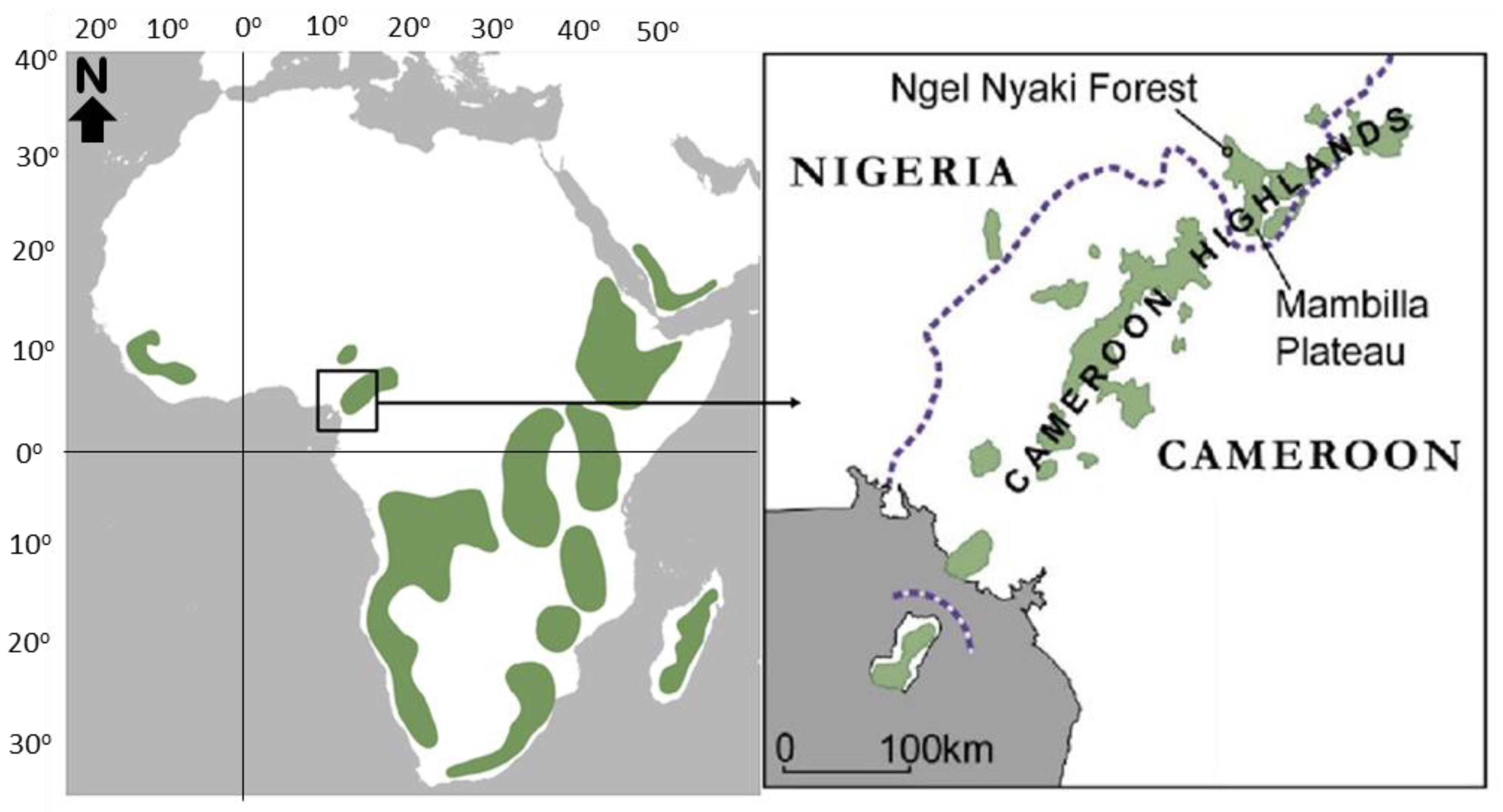
Figure 1.
Location of the Ngel Nyaki Forest, on the Mambilla Plateau, Nigeria relative to the approximate distribution of other major montane ecosystems in Africa, shown in green [31]. The forest lies close to the Nigeria/Cameroon border, represented by a dashed purple line.
Figure 1.
Location of the Ngel Nyaki Forest, on the Mambilla Plateau, Nigeria relative to the approximate distribution of other major montane ecosystems in Africa, shown in green [31]. The forest lies close to the Nigeria/Cameroon border, represented by a dashed purple line.

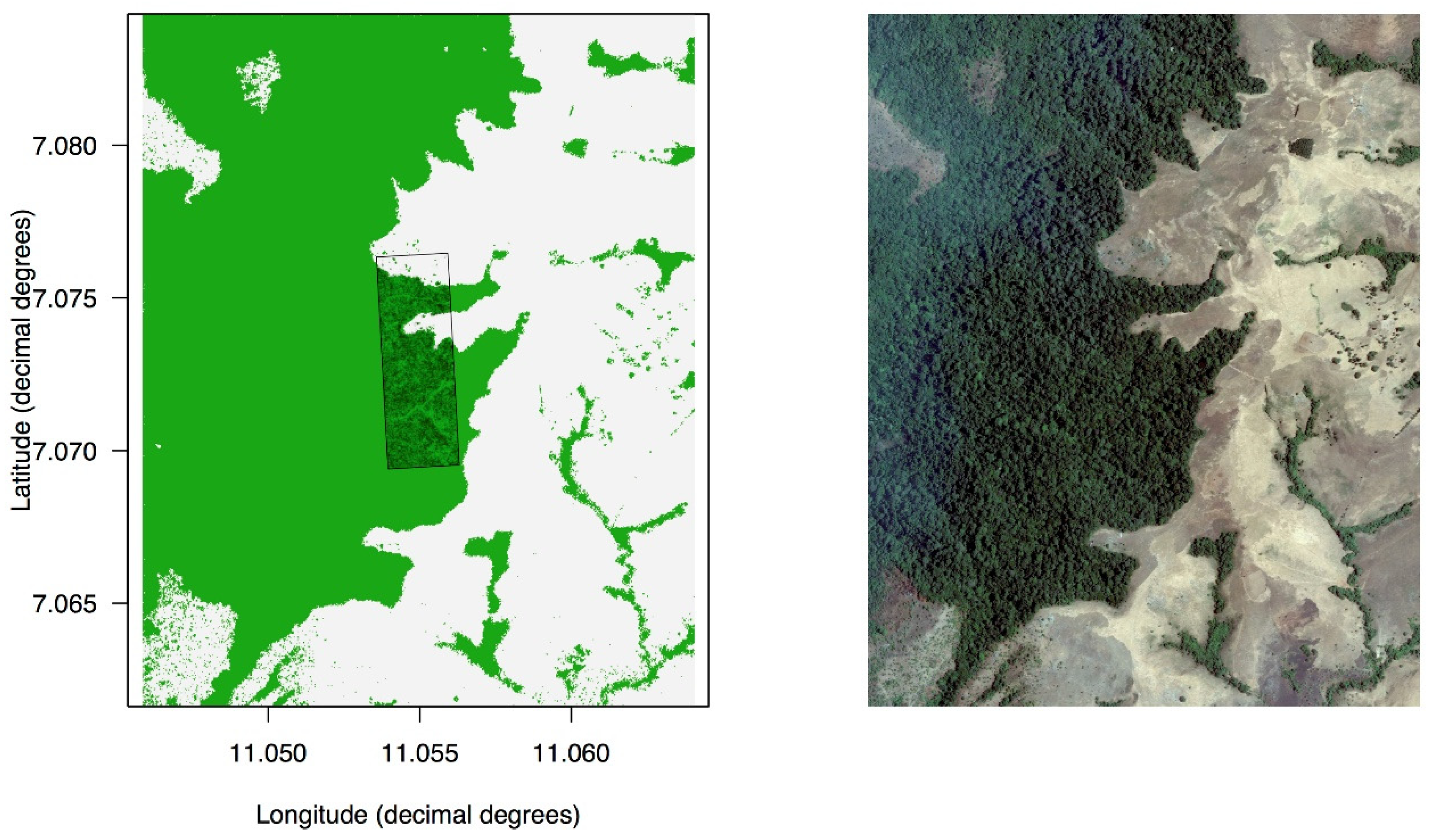
Figure 2.
Vegetation mosaic in the Ngel Nyaki Forest Dynamics Plot (260 × 780 m) and surrounding areas. White pixels are grass, green pixels are forest. The location of the plot is shown by the black rectangle on the simplified vegetation map on the left (A). For the purposes of this study, “grass” was defined as pixels with red content 37% or more in a jpg image of the area taken from Google Earth, presented on the right (B). This 37% threshold was optimized to obtain the best possible correspondence between the aerial image and the binary map of the grass/forest boundary. Pixels are approximately 1 × 1 m, allowing for an individual tree-level resolution. This allowed the fine-tuning of the geolocation of the plot to obtain an almost perfect match between our individual tree map (trees within the plot) and the larger grass vs. forest map.

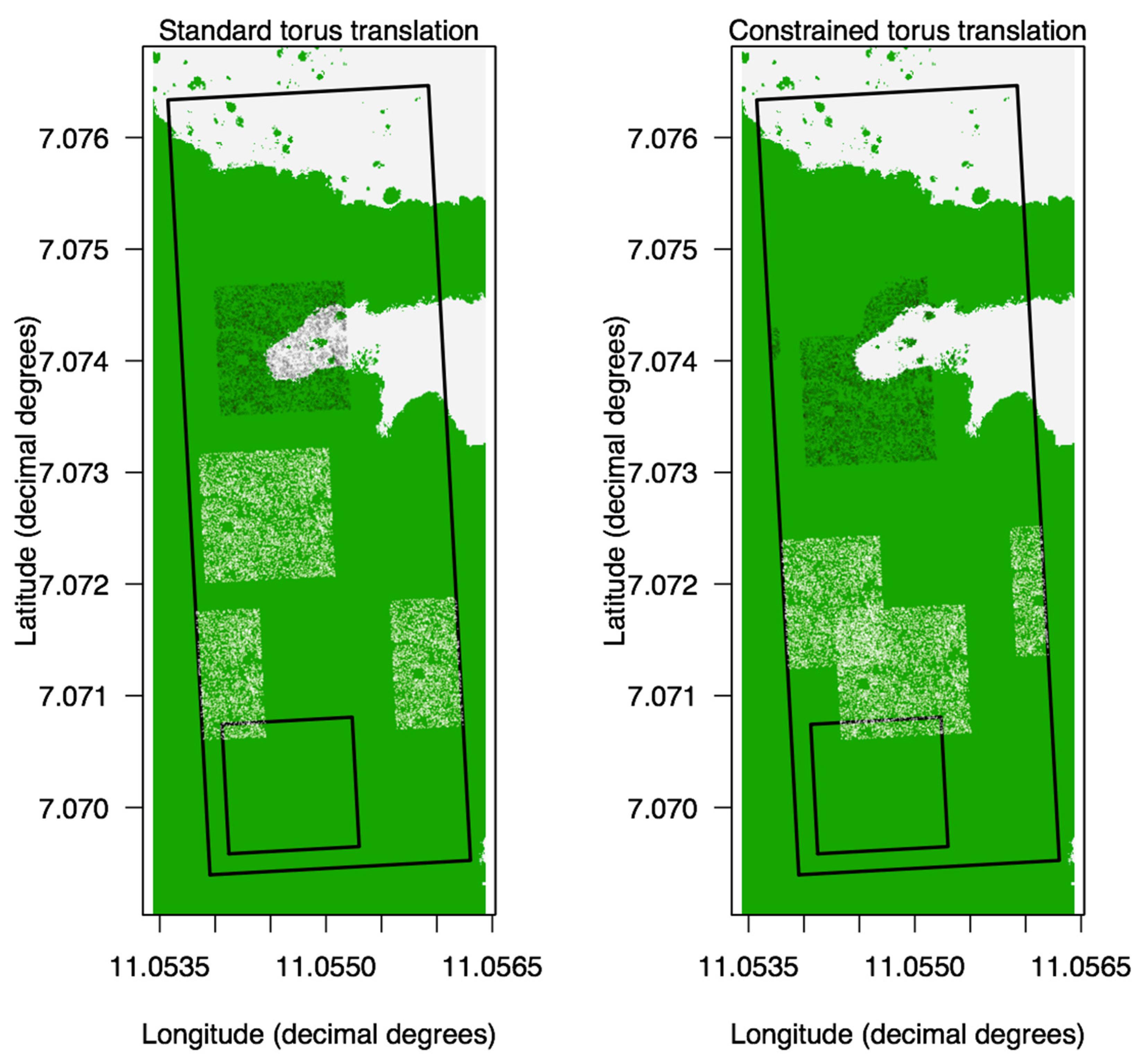
Figure 3.
Comparison between the standard (unconstrained) torus translation (A) and the constrained version that we used in our study (B). The square polygon within the plot corresponds to the original position of a subset of stems, used as an example. Three random translations of this subset of stems are presented for comparison purposes. When the stems land within forest after the translation, both methods behave similarly (whitish points). When the stems land within grass, the constrained translation makes them “jump” again until they find forest, distorting to some degree the translated cloud of points (black points). The standard (unconstrained) translation does nothing in particular, since it is blind to the forest vs. grass distinction. This non-adaptive behavior of the standard torus translation contributes to the unrealistic null expectation of “many stems within the grass”, that we wanted to avoid.

Figure 4.
Distribution of individual trees along the four environmental gradients in the Ngel Nyaki plot. Individual trees occur across all gradients, therefore our analysis reflects the underlying correlation between individuals and measured local environmental variables. For computational reasons, the distance to the grass was measured with high resolution at short distances and coarser resolution at larger distances (the maximum peripheral error was constrained to <15%). The possible values for the distance to the grass are represented by thin grey lines in the figures; the points have been jittered around those possible values for visualization purposes.

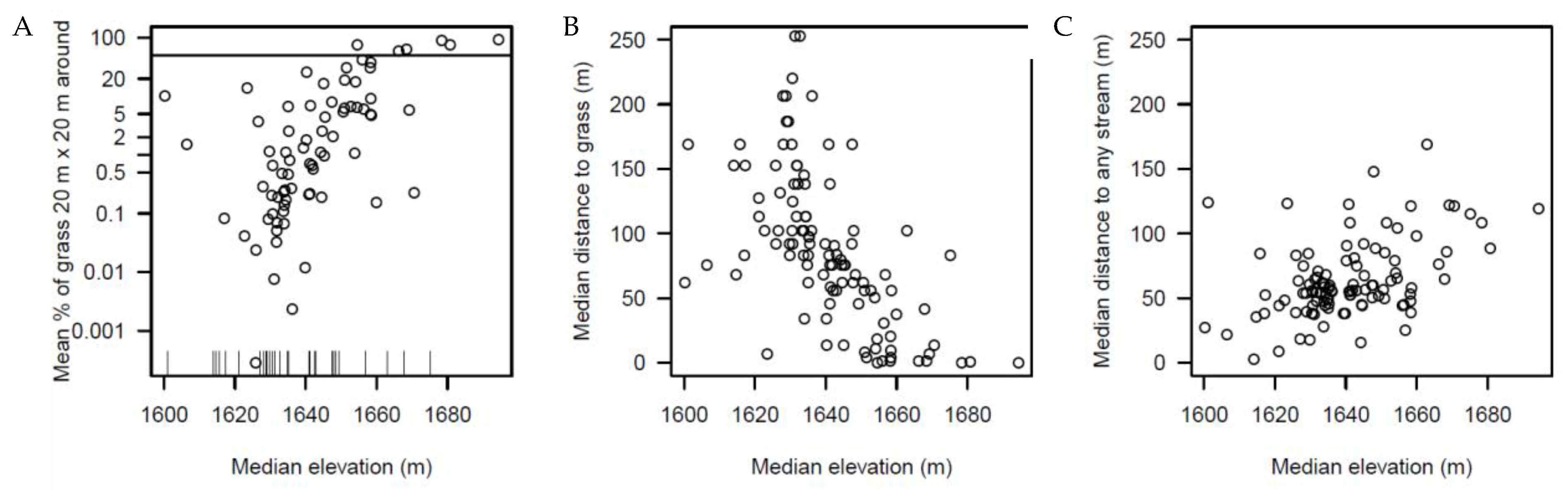
Figure 5.
Environmental preferences of species in the Ngel Nyaki plot. Each point in the figure represents one species. (A) Median elevation of the individuals of each species vs. the mean % of grass pixels in a 20 × 20 m window around each individual of the species (r = 0.57). The vertical axis is in logarithmic scale; ticks in the horizontal axis represent species that have absolutely no grass around (zeroes cannot be represented in the logarithmic scale). The horizontal line at 50% separates four savannah species and two species from the rest. (B) Median elevation vs. median distance to the grass across all the individuals of each species (r = −0.60). (C) Median elevation vs. median distance to the closest stream across all the individuals of each species (r = 0.45).


Table 1.
Tree abundance and diversity in the 20.28-ha Ngel Nyaki Plot, in three diameter at breast height (dbh) categories. Mean values and standard deviations are presented for per hectare estimates.
Table 1.
Tree abundance and diversity in the 20.28-ha Ngel Nyaki Plot, in three diameter at breast height (dbh) categories. Mean values and standard deviations are presented for per hectare estimates.
| Variables | dbh ≥ 1 cm | dbh ≥ 10 cm | dbh ≥ 30 cm |
|---|---|---|---|
| Number of species | 105 | 88 (83%) | 61 (58%) |
| Number of genera | 88 | 76 (86%) | 56 (64%) |
| Number of families | 47 | 43 (92%) | 34 (72%) |
| Abundance | 41,031 | 6931 (17%) | 1686 (4%) |
| Total basal area (m2) | 553.49 | 498.24 (90.0%) | 356.60 (64%) |
| Fisher’s α per hectare | 12.42 ± 1.51 | 12.03 ± 2.20 | 9.55 ± 2.74 |
| Mean density per hectare (N/ha) | 2061.86 ± 697.03 | 351.79 ± 112.74 | 85.04 ± 28.00 |
| Mean basal area per hectare (m2/ha) | 27.52 ± 8.64 | 24.70 ± 7.87 | 17.62 ± 5.58 |
Table 2.
The twenty most abundant woody plant species in the Ngel Nyaki plot, ranked by density. The rank corresponding to their basal area is indicated in parentheses.
Table 2.
The twenty most abundant woody plant species in the Ngel Nyaki plot, ranked by density. The rank corresponding to their basal area is indicated in parentheses.
| Species | Family | Density (Trees/ha) | Basal Area (m2/ha) |
|---|---|---|---|
| Garcinia smeathmanii (Planch. & Triana) Oliv. | Clusiaceae | 607.63 | 1.20 (7) |
| Deinbollia pinnata Schumach. &Thonn. | Sapindaceae | 158.68 | 0.49 (11) |
| Pleiocarpa pycnantha (K.Schum.) Stapf | Apocynaceae | 107.51 | 0.48 (12) |
| Leptaulus zenkeri Engl. | Icacinaceae | 69.19 | 1.25 (6) |
| Carapa oreophila Kenfack | Meliaceae | 56.92 | 2.14 (3) |
| Chrysophyllum albidum G. Don | Sapotaceae | 56.75 | 0.21 (18) |
| Sorindeia sp. | Anacardiaceae | 53.10 | 0.25 (15) |
| Strombosia scheffleri Engl. | Olacaceae | 51.13 | 2.76 (2) |
| Drypetes gosweilleri S. Moore | Putranjivaceae | 50.42 | 0.63 (10) |
| Newtonia buchannani (Baker f.) G.C.C. Gilbert & Boutique | Fabaceae | 47.95 | 0.87 (8) |
| Dicranolepis grandiflora Engl. | Thymelaeceae | 47.54 | 0.04 (19) |
| Anthonotha noldeae (Rossberg) Exell and Hillc. | Fabaceae | 46.24 | 3.42 (1) |
| Voacanga africana Stapf | Apocynaceae | 44.52 | 0.22 (17) |
| Tabernaemontana contorta Stapf | Apocynaceae | 40.38 | 0.23 (16) |
| Santiria trimera (Oliv.) Aubrév. | Burseraceae | 40.36 | 1.76 (4) |
| Oxyanthus speciosus DC. | Rubiaceae | 39.21 | 0.47 (13) |
| Psychotria peduncularis (Salisb.) Steyerm. | Rubiaceae | 37.58 | 0.01 (20) |
| Macaranga occidentalis (Müll. Arg.) Müll. Arg. | Euphorbiaceae | 34.90 | 0.84 (9) |
| Trichilia monadelpha (Thonn.) J.J. de Wilde | Meliaceae | 28.18 | 1.40 (5) |
| Millettia conraui Harms | Fabaceae | 23.04 | 0.27 (14) |
Table 3.
Associations between the distribution of the common species and four environmental gradients in the Ngel Nyaki plot (Nigeria). The numeric values correspond to the proportion of null values (medians across individuals, except in the case of % of surrounding grass, which are means) that are lower than the observed value. The columns “association” contain a short label for the ecological interpretation of the results: forest vs. savannah species, edge vs. core species (core = species that are significantly far from the grass), species that prefer low vs. high elevations, and species that prefer being close to the streams (wet) or far from them (dry). NA’s mean that a given association does not deviate significantly from the expected by the null model. We include species guild, growth form, seed size, and dispersal mode (Growth-form categories of species were ET = emergent tree, CT = canopy tree, UT = understory tree, USh = understory shrub, ST = savannah tree, Sh = shrub (modified from [27]). Species shade tolerance guilds included P = pioneer, S = shade-tolerant, CP = Cryptic pioneer, NPLD= Non-pioneer light demanding, G = Grassland (modified from [35]). Dashes (-) signify insufficient data).
| Species | % of Grass in 20 × 20 m Around | Distance to the Grass | Elevation | Distance to Streams | Guild | Growth Form | Seed Size (g) | Dispersal Mode | ||||
|---|---|---|---|---|---|---|---|---|---|---|---|---|
| Prop. of obs. > Null | Association | Prop. of obs. > Null | Association | Prop. of obs. > Null | Association | Prop. of obs. > Null | Association | |||||
| Leptaulus zenkeri | 0 | forest | 1 | core | 0.159 | NA | 0.47 | NA | S | CT | 0.12 | animal |
| Newtonia buchanannii | 0 | forest | 1 | core | 0.272 | NA | 0.157 | NA | S | ET | 0.14 | wind |
| Chrysophylum albidum | 0 | forest | 0.998 | core | 0.143 | NA | 0.818 | NA | S | CT | 0.35 | animal |
| Voacanga africana | 0 | forest | 0.992 | core | 0.154 | NA | 0.518 | NA | S | UT | 0.24 | animal |
| Dicranolepis grandifolia | 0 | forest | 0.992 | core | 0.157 | NA | 0.51 | NA | S | UT | 0.38 | animal |
| Chionanthus africanus | 0 | forest | 0.989 | core | 0.144 | NA | 0.988 | dry | S | CT | - | animal |
| Drypetes gossweileri | 0 | forest | 0.978 | core | 0.133 | NA | 0.028 | wet | S | CT | 0.01 | animal |
| Oxyanthus speciosus | 0 | forest | 0.975 | core | 0.326 | NA | 0.726 | NA | S | UT | 1.60 | animal |
| Pavetta corymbosa | 0 | forest | 0.974 | core | 0.479 | NA | 0.495 | NA | S | USh | 0.02 | animal |
| Discoclaoxylon hexandrum | 0 | forest | 0.963 | core | 0.119 | NA | 0.843 | NA | S | USh | 0.04 | animal |
| Campylospermum flavum | 0 | forest | 0.961 | core | 0.234 | NA | 0.035 | wet | S | UT | - | animal |
| Dasylepis racemosa | 0 | forest | 0.925 | NA | 0.680 | NA | 0.441 | NA | S | UT | 0.43 | animal |
| Santiria trimera | 0 | forest | 0.922 | NA | 0.024 | low | 0.085 | NA | S | CT&UT | 1.32 | animal |
| Garcinia smeathmannii | 0 | forest | 0.905 | NA | 0.141 | NA | 0.712 | NA | S | UT | 2.57 | animal |
| Strombosia scheffleri | 0 | forest | 0.872 | NA | 0.027 | low | 0.099 | NA | S | CT | - | animal |
| Trichilia monadelpha | 0 | forest | 0.862 | NA | 0.220 | NA | 0.046 | wet | S | CT | 0.50 | animal |
| Sapium ellipticum | 0 | forest | 0.841 | NA | 0.121 | NA | 0.014 | wet | P | CT | - | animal |
| Diospyros monbuttensis | 0 | forest | 0.743 | NA | 0.353 | NA | 0.913 | NA | S | UT | 0.68 | animal |
| Kigellia africana | 0 | forest | 0.606 | NA | 0.272 | NA | 0.397 | NA | NPLD | CT | - | animal |
| Psychotria peduncularis | 0 | forest | 0.547 | NA | 0.263 | NA | 0.831 | NA | P | USh | 0.03 | animal |
| Antidesma vogelianum | 0 | forest | 0.515 | NA | 0.196 | NA | 0.675 | NA | P | USh | 0.03 | animal |
| Trilepisium madagascariense | 0 | forest | 0.451 | NA | 0.479 | NA | 0.640 | NA | - | CT | 0.97 | animal |
| Symphonia globulifera | 0 | forest | 0.444 | NA | 0.056 | NA | 0.409 | NA | S | CT | 0.45 | animal |
| Polyscias fulva | 0 | forest | 0.442 | NA | 0.228 | NA | 0.536 | NA | P/CP | UT | 0.01 | animal |
| Celtis gomphophylla | 0 | forest | 0.430 | NA | 0.154 | NA | 0.662 | NA | P/CP | UT | 0.01 | animal |
| Carapa oreophila | 0 | forest | 0.411 | NA | 0.032 | low | 0.063 | NA | NPLD | UT | 18.51 | gravity |
| Xymalos monospora | 0 | forest | 0.398 | NA | 0.667 | NA | 0.172 | NA | S | UT | 0.17 | animal |
| Parkia filicoidea | 0 | forest | 0.355 | NA | 0.048 | low | 0.939 | NA | NPLD | CT | 0.77 | animal |
| Mallotus oppositifolius | 0 | forest | 0.317 | NA | 0.418 | NA | 0.115 | NA | S | USh | 0.02 | animal |
| Zanthoxylum leprieurii | 0 | forest | 0.215 | NA | 0.803 | NA | 0.540 | NA | CP | UT | 0.02 | animal |
| Ficus sur | 0 | forest | 0.211 | NA | 0.351 | NA | 0.165 | NA | Strangler | Strangler | - | animal |
| Leea guineensis | 0 | forest | 0.202 | NA | 0.620 | NA | 0.569 | NA | CP | USh | 0.04 | animal |
| Psychotria succulenta | 0 | forest | 0.189 | NA | 0.358 | NA | 0.855 | NA | P | USh | - | animal |
| Trema orientalis | 0 | forest | 0.169 | NA | 0.011 | low | 0.236 | NA | P/ CP | UT | 0.01 | animal |
| Nuxia congesta | 0 | forest | 0.167 | NA | 0.017 | low | 0.382 | NA | P | UT | <0.001 | animal |
| Albizia gummifera | 0 | forest | 0.136 | NA | 0.980 | high | 0.664 | NA | P/CP | CT | 0.55 | wind |
| Entandophragma angolense | 0 | forest | 0.133 | NA | 0.063 | NA | 0.885 | NA | NPLD | ET | 1.73 | wind |
| Macaranga occidentalis | 0 | forest | 0.107 | NA | 0.327 | NA | 0.008 | wet | P | UT | 0.01 | animal |
| Deinbollia pinnata | 0 | forest | 0.104 | NA | 0.855 | NA | 0.841 | NA | S | UT | 0.62 | animal |
| Pouteria altissima | 0 | forest | 0.103 | NA | 0.833 | NA | 0.226 | NA | NPLD | ET | 3.19 | animal |
| Ficus lutea | 0 | forest | 0.051 | NA | 0.729 | NA | 0.213 | NA | Strangler | Strangler | - | animal |
| Pleiocarpa pycnantha | 0 | forest | 0.030 | edge | 0.892 | NA | 0.530 | NA | S | UT | 0.25 | animal |
| Beilschmiedia mannii | 0 | forest | 0.013 | edge | 0.816 | NA | 0.464 | NA | S | UT | 1.16 | animal |
| Isolona sp. | 0 | forest | 0.010 | edge | 0.870 | NA | 0.649 | NA | S | UT | 1.62 | animal |
| Millettia conraui | 0 | forest | 0.007 | edge | 0.796 | NA | 0.326 | NA | P/CP | UT | 0.20 | ballistic |
| Warneckea cinnamomoides | 0 | forest | 0.005 | edge | 0.664 | NA | 0.623 | NA | P/CP | USh | - | animal |
| Rauvolfia vomitoria | 0 | forest | 0.002 | edge | 0.520 | NA | 0.829 | NA | P/CP | USh | 0.07 | animal |
| Rothmania urcelliformis | 0 | forest | 0.002 | edge | 0.999 | high | 0.551 | NA | S | UT | 0.31 | animal |
| Eugenia gilgii | 0 | forest | 0.001 | edge | 0.806 | NA | 0.457 | NA | P | UT | 0.11 | animal |
| Ritchiea albersii | 0 | forest | 0.001 | edge | 0.996 | high | 0.774 | NA | S | UT | - | animal |
| Clausena anisata | 0 | forest | 0 | edge | 0.966 | high | 0.783 | NA | P/CP | USh | 0.07 | animal |
| Sorindeia sp. | 0 | forest | 0 | edge | 0.754 | NA | 0.713 | NA | NPLD | CT | 0.30 | animal |
| Tabanaemontana contorta | 0 | forest | 0 | edge | 0.971 | high | 0.922 | NA | P/CP | UT | 0.35 | animal |
| Anthonotha noldeae | 0 | forest | 0 | edge | 0.968 | high | 0.696 | NA | P/CP | CT | 6.57 | ballistic |
| Bridelia speciosa | 0 | forest | 0 | edge | 0.510 | NA | 0.847 | NA | P/CP | UT | - | wind |
| Ficus sp. | 0 | forest | 0 | edge | 0.945 | NA | 0.440 | NA | Strangler | Strangler | - | animal |
| Psychotria umbellata | 0 | forest | 0 | edge | 0.602 | NA | 0.923 | NA | P | USh | - | animal |
| Guarea cedrata | 0 | forest | 0 | edge | 0.300 | NA | 0.896 | NA | P/CP | UT | - | animal |
| Psorospermum aurantiacum | 1 | savanna | 0 | edge | 0.751 | NA | 0.907 | NA | G | Sh | 0.01 | animal |
| Entada abyssinica | 1 | savanna | 0 | edge | 0.999 | high | 0.852 | NA | G | ST | 0.25 | wind |
| Dombeya ledermannii | 1 | savanna | 0 | edge | 0.840 | NA | 0.467 | NA | G | ST | - | ballistic |
| Rytigynia sp. | 1 | savanna | 0 | edge | 0.797 | NA | 0.804 | NA | G | Sh | - | animal |
| Rubiaceae unidentified | 0 | forest | 0.998 | core | 0.359 | NA | 0.518 | NA | S | UT | - | animal |
| Unidentified | 0 | forest | 0.033 | edge | 0.475 | NA | 0.553 | NA | - | - | - | |
| Unidentified | 0 | forest | 0.002 | edge | 0.997 | high | 0.350 | NA | P | U | - | |
© 2020 by the authors. Licensee MDPI, Basel, Switzerland. This article is an open access article distributed under the terms and conditions of the Creative Commons Attribution (CC BY) license (http://creativecommons.org/licenses/by/4.0/).
Share and Cite
MDPI and ACS Style
Abiem, I.; Arellano, G.; Kenfack, D.; Chapman, H. Afromontane Forest Diversity and the Role of Grassland-Forest Transition in Tree Species Distribution. Diversity 2020, 12, 30. https://0-doi-org.brum.beds.ac.uk/10.3390/d12010030
AMA Style
Abiem I, Arellano G, Kenfack D, Chapman H. Afromontane Forest Diversity and the Role of Grassland-Forest Transition in Tree Species Distribution. Diversity. 2020; 12(1):30. https://0-doi-org.brum.beds.ac.uk/10.3390/d12010030
Chicago/Turabian StyleAbiem, Iveren, Gabriel Arellano, David Kenfack, and Hazel Chapman. 2020. "Afromontane Forest Diversity and the Role of Grassland-Forest Transition in Tree Species Distribution" Diversity 12, no. 1: 30. https://0-doi-org.brum.beds.ac.uk/10.3390/d12010030
Note that from the first issue of 2016, this journal uses article numbers instead of page numbers. See further details here.