
N90, a Diversity Index Sensitive to Variations in Beta Diversity Components


Centre Oceanogràfic de les Balears, Instituto Español de Oceanografía, Moll de Ponent s/n, 07015 Palma, Spain
*
Author to whom correspondence should be addressed.
Diversity 2021, 13(10), 489; https://0-doi-org.brum.beds.ac.uk/10.3390/d13100489
Submission received: 31 August 2021
/
Revised: 25 September 2021
/
Accepted: 30 September 2021
/
Published: 6 October 2021
Abstract
:Species diversity in a community is mainly related to the number and abundance of species that form it. N90 is a recently developed diversity index based on the results of the similarity percentage (SIMPER) analysis that represents the number of species contributing up to ninety percent of within-group similarity in a group of samples. The calculation of N90 is based on the Bray–Curtis similarity index and involves the number of species and abundances in a group of samples. We have explored the properties of N90 compared to other alpha, beta and gamma diversity indices and to beta diversity measures accounting for nestedness and turnover. We have used a non-real data set to compare the values of all indices with N90 and two real data sets of demersal fish communities along large and short depth gradients with higher influence of turnover and nestedness, respectively, to correlate the same indices with N90. The sensitivity of N90 to reductions in the frequency of occurrence and the evenness of the distribution of species abundances among samples allows the detection of diversity loss due to the fishing-induced retreatment of species populations to localities presenting the most favorable ecological conditions. This property, both in the identification of species replacement and species loss through SIMPER analysis, make N90 a useful indicator to support the Ecosystem Approach to Fisheries within the current context of global change.
1. Introduction
Diversity is a founding, but at the same time, complex concept in ecology. More than species diversity in the community, understood as a group of interdependent organisms of different species growing or living together in a specified habitat, diversity can be related to genetic diversity within populations or diversity of functional traits. However, for most ecologists, diversity has to do with the number and abundance of species in the community, and a lot of attempts have been made to express this concept numerically. Because of this, a high number of diversity indices have been proposed showing different aspects of the community structure, taking into account factors ranging from the number of species and the relative abundance or biomass of these species, to the taxonomic or functional relationships between them [1]. Although it is generally agreed that diversity is a multidimensional concept and that the use of diversity indices depends on what effect on diversity you want to detect, there is no consensus about the indices that should be used in each case. However, traditional or classical diversity indices such as Species Richness (S), Shannon (H′) or Pielou’s evenness (J′), are usually chosen to describe biological communities because, at least, they are easy to calculate and allow comparisons with previous works. Although in recent years, a new family of diversity indices, known as Hill numbers, have been preferred because they have shown more desired properties than the raw form [2,3]; for example, they obey an intuitive replication principle or doubling property and they are all expressed in units of effective numbers of species [4].
Taking into account changes of diversity along transects or across environmental gradients, the concept of beta diversity emerges. Although there is some controversy [5,6], it is generally agreed that beta diversity measures the species that change between samples or sites composing a community, mainly due to species replacement or species loss [7]. The concept of beta diversity was originally proposed by Whittaker [8,9], and their measures were summarized by Chao and Chiu [10] in two major approaches: (i) the diversity decomposition approach that consists of decomposing the total diversity (gamma) into its within-community component (alpha) and between-community component (beta), which can be applied to species richness as well as to other diversity indices involving abundances in their calculations; and (ii) the variance framework approach that includes various factors from clustering or ordination analysis to dissimilarity measures between pairs of sites (e.g., [5,11,12]) to compute beta diversity. Moreover, dissimilarity indices allow the distinction of species loss (or nestedness) and species replacement (or turnover) components of beta diversity and can be extended to multiple-site measures [7].
N90 is a diversity index developed by Farriols et al. [13], based on the results of the Similarity Percentage (SIMPER) analysis [14]. This analysis takes into account the similarity in species composition between pairs of samples of a group to calculate the average similarity within the group (or within-group similarity). The N90 index represents the number of species contributing up to the 90% of within-group similarity in a group of samples, based on the calculation of the contribution of each species. Like SIMPER analysis N90 uses the Bray–Curtis similarity index as proposed by Clarke [14]. Following the variance framework, within-group similarity could be interpreted as an inverse measure of beta diversity. The hypothesis behind the N90 index is that impacted communities may see both the frequency of occurrence and the evenness of the distribution of species abundances reduced among samples. This leads to a decrease in N90 due to the retreat of species populations to the localities presenting the most favorable ecological conditions.
The aim of this work is to explore the properties of N90 compared to other diversity indices involving number of species and abundance in their calculation. To do so we compared N90 to classical diversity indices and their alpha, gamma and beta versions. Following the variance framework approach, we have also compared N90 to beta diversity measures accounting for nestedness and turnover and to within-group similarity from SIMPER analysis. We have used a non-real data set with several groups of samples showing different values of abundance distributions and number of species between samples to compare the values of all indices with N90. We have also used two real data sets of demersal fish communities along large and short depth gradients with higher influence of turnover and nestedness, respectively, to correlate the same indices with N90.
2. Materials and Methods
2.1. Background Calculation
The N90 is based on the SIMPER analysis that quantifies the contribution of each species to the within-group similarity in a group of samples. This analysis starts with the calculation of the Bray–Curtis similarity index [15] as proposed by Clarke [14]:
where yij is the abundance of the species i in the sample j; yik is the abundance of the species i in the sample k; p is the total number of species in j and k; and min (yij, yik) is the minimum value of the abundance of species i between the samples j and k, taking zero into account. The contribution of each species i to the total similarity of the group Si is the mean value of Sjk (i) for a species in all the sample comparisons in the group. As a result, the total similarity in a group (Sim) is the sum of Si for all the species in the group:
Then the contribution of Si to Sim is rescaled to 100% and the species are arranged in decreasing order.
2.2. N90 Index
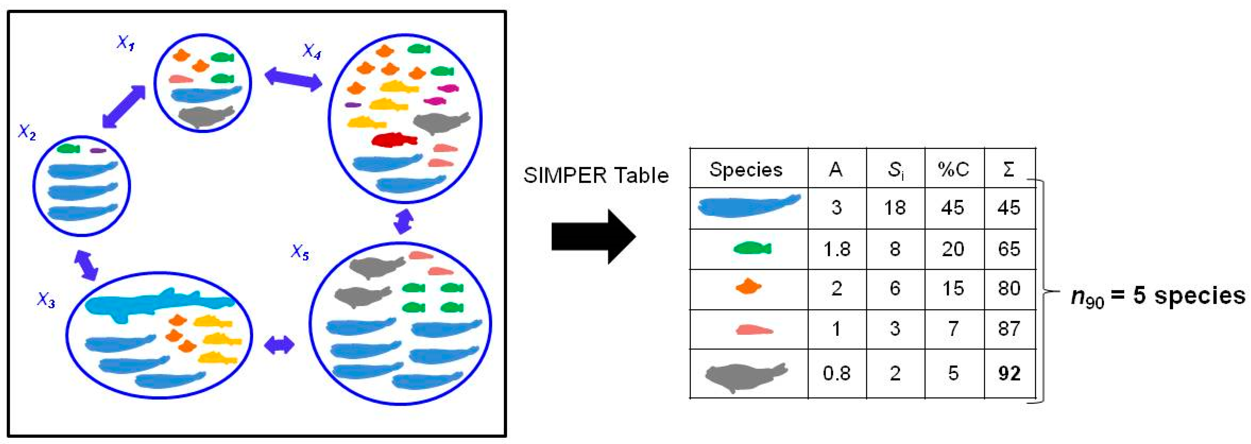
The N90 index is based on the SIMPER analysis and the calculations already explained in Section 2.1. Once the contribution of Si to Sim is rescaled to 100% and the species are arranged in decreasing order, the number of species that contributes up to 90% of within-group similarity is obtained (n90; Figure 1).
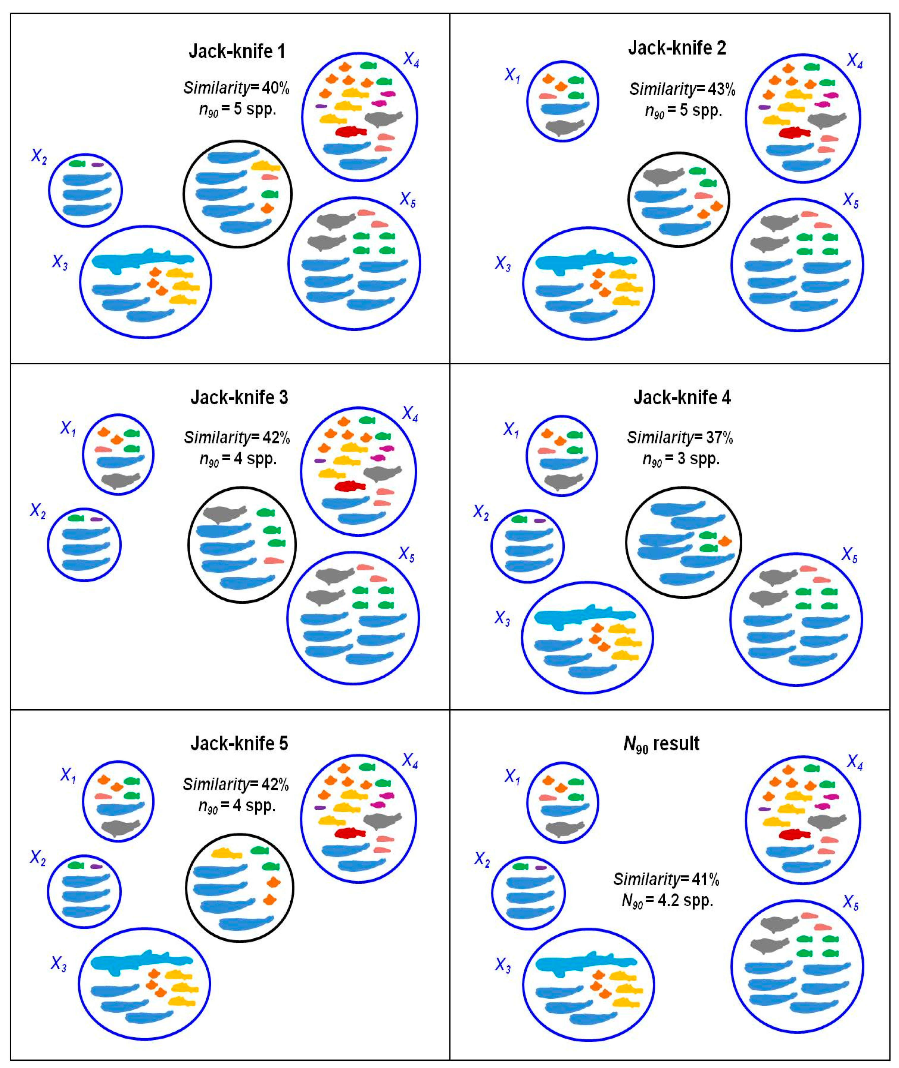
This procedure is done for each re-sampling in a jack-knife routine, which removes a sample each time, in order to obtain the average and the dispersion value for the group of samples analyzed. At the end of the procedure, there are as many lists of contribution to similarity by species as number of re-samplings. The N90 diversity index is the mean number of species which accumulates up to 90% of within-group similarity in all the re-samplings (mean n90; Figure 2). In Appendix A we introduce the script developed to calculate N90 in R, version 4.4.1 [16], and the use of the script and their main functions are explained. Vegan package [17] is required to carry out all the analyses.
2.3. Diversity Decomposition Approach
Following the multiplicative partitioning approach [6], alpha, beta and gamma versions of S, H′, Hill number of order 1 (H1), J′ and J1 were calculated to frame N90 in alpha, beta or gamma components of diversity. S is the raw number of species in each haul and H′, H1, J′ and J1 were calculated as follows:
where pi is the proportion of all individuals belonging to species i and S is the total number of species in the sample.
In the case of S: (i) alpha diversity was calculated as the mean number of species among the samples of each group; (ii) gamma diversity was calculated as the total number of species for the whole group; and (iii) beta diversity was calculated as gamma diversity divided by alpha diversity. Similarly, alpha, beta and gamma versions of H′, H1, J′ and J1 were calculated: (i) alpha diversity was calculated as the mean value of each index among all the samples in each group; (ii) gamma diversity was calculated from the mean values of abundances for each species in the group of samples and then calculation of each diversity index for the whole group; and (iii) beta diversity was calculated as gamma diversity divided by alpha diversity.
Once all the indices were calculated, we correlated the values of N90 to alpha, beta and gamma versions of S, H′, H1, J′ and J1 by means of linear regression analysis.
2.4. Variance Framework Approach
We have calculated three multiple-site beta diversity measures. These measures are derived from the pair-wise dissimilarity indices of Sørensen [18,19], Simpson [19,20,21] and nestedness [7]. They have been chosen because, like their pair-wise analogs, they are able to distinguish the main causes of change in beta diversity: species replacement or turnover and species loss or nestedness between sites of a community. While the Sorensen-based multiple site dissimilarity index (βSOR) [7] accounts for both species turnover and nestedness, the Simpson-based multiple site dissimilarity (βSIM) [7] only accounts for species turnover. The multiple-site dissimilarity measure of nestedness (βNES) [7] is derived from simple subtraction as follows:
where Si is the total number of species in a site i; ST is the total number of species considered in all sites together; and bij, bji are the number of species exclusive to site i and j, respectively. All the indices were calculated in R, version 4.4.1 [16], with functions developed by Baselga [7].
Within-group similarity has also been included in the analysis as an inverse measure of beta diversity, because, like N90, it includes abundances of species in its calculation (see Section 2.1).
When all the indices were calculated, and due to the non-constant variance of residuals, we assessed the correlation of the values of N90 with all the indices from Section 2.3 and Section 2.4 through the Spearman’s rank correlation coefficient (ρ).
2.5. Non-Real Data Set
A non-real data set available in the Supplementary Materials data was used to explore the properties of N90. The data set is in two files (‘nonreal_sp.csv’ and ‘nonreal_group.csv’) and its use is analogous to the data set used as an example in Appendix A. The 12 groups of samples created (A-L) take into account changes in abundance distributions and number of species between samples. All the groups contain 10 samples. Abundances of species are 10 in all cases, except when it is indicated in the group, and are distributed as follows:
- Group A: Maximum similarity; 20 species equally abundant in all samples with abundance of 10.
- Group B: Maximum similarity and lower abundance than group A; 20 species equally abundant in all samples with abundance of 5.
- Group C: Disappearance of 50% of abundance of 50% of species in all samples; 10 species are equally abundant in all samples with an abundance of 10 and 10 species are equally abundant in all samples with an abundance of 5.
- Group D: Disappearance of 50% of species in all samples; 10 species are equally abundant in all samples with an abundance of 10 and 10 species have disappeared from all samples.
- Group E: Reduction of 50% in abundance of all species in 50% of samples; All species are equally abundant in 5 samples with an abundance of 5 and in 5 samples with an abundance of 10.
- Group F: Disappearance of 25% of species from all samples and reduction of 50% of abundance in 25% of species; 10 species are equally abundant in all samples with an abundance of 10, 5 species are equally abundant in all samples with an abundance of 5 and 5 species have disappeared from all samples.
- Group G: Each sample presents a subset of species of the previous one, with abundances of 10.
- Group H: Each sample presents a subset of species of the previous one, with abundances of 10, but with a higher number of species than in group G.
- Group I: There is species loss and replacement between samples, with abundances of 10
- Group J: There is lower species loss and replacement between samples than group I, with abundances of 10.
- Group K: Same species loss and replacement between samples as J, with abundances of 5 in some samples.
- Group L: Higher species loss and lower replacement of species between samples than group J.
All the indices from Section 2.3 and Section 2.4 have also been calculated for all the groups of samples to compare the results with N90.
2.6. Real Data Set
Data collected during the International Bottom Trawl Survey in the Mediterranean (MEDITS) on demersal fish communities of the Balearic Islands was used to correlate N90 with diversity indices from Section 2.3 and Section 2.4. The characteristics of the sampling gear and protocols are explained in detail by Spedicato et al. [22]. This scientific survey has been conducted annually since 2001 during late spring in the Balearic Islands, covering the soft bottoms of the continental shelf and slope between 50 and 800 m depth. According to the MEDITS protocol, four depth strata were taken into account: (i) shallow shelf from 50 to 100 m; (ii) deep shelf from 101 to 200 m; (iii) upper slope from 201 to 500 m; and (iv) middle slope from 501 to 800 m. A total of 650 hauls (around 50 per year) carried out between 2002 and 2015 were analyzed. In each haul, fish species were sorted and individuals were counted and weighed. Abundances of fish species were standardized to one square km, using the horizontal opening of the net and the distance covered in each haul, obtained using the SCANMAR system and Global Positioning System (GPS), respectively. Markedly pelagic or mesopelagic species were excluded from the analysis.
The groups of samples considered for the calculation of all the indices, including N90, were defined by the MEDITS depth strata and the sampling year. Depth is a factor that highly structures demersal fish communities, with a high grade of species replacement along a depth gradient. As such, a high influence of turnover is expected when considering long depth gradients, like the four depth strata sampled during MEDITS surveys (50–800 m). Therefore, we have also restricted the analysis to the stratum showing higher values of nestedness (βNES) to consider shorter depth gradients less influenced by turnover than larger ones. In this case, a homogeneous community along a time series is considered and species loss is more relevant than species replacement. The treatment of both sets of samples will allow us to better distinguish the weight of both components of beta diversity, turnover and nestedness, in the calculation of N90.
3. Results
3.1. Non-Real Data
Results of N90 and all the indices of alpha, beta and gamma diversity considered for the non-real data set are presented in Table 1 and Table 2. N90 showed the highest values (N90 = 18) in groups A, B and E, where alpha H′ and alpha H1 also showed the highest value (alpha H′ = 3; alpha H1 = 20) and the lowest (N90 = 9) in group D, where gamma S was also the lowest (gamma S = 10) from all groups. N90 decreased when abundances of 50% of species decreased to 50% (group A compared to C), but did not change when all abundances reduced to 50% (groups A compared to B). N90 was lower in F compared to C and higher compared to D. N90 was lower in group G where nestedness (βNES = 0.65) was higher than in group H (βNES = 0.38). N90 was also lower in group I (βSOR = 0.74, βSIM = 0.61 and βNES = 0.12) compared to group J (βSOR = 0.70, βSIM = 0.59 and βNES = 0.10), where evenness and turnover were lower. N90 was higher in J (N90 = 14.6) compared to K (N90 = 14.4). N90 decreased in group L (N90 = 13.4) where the turnover took a low value (βSIM = 0.32).
3.2. Real Data
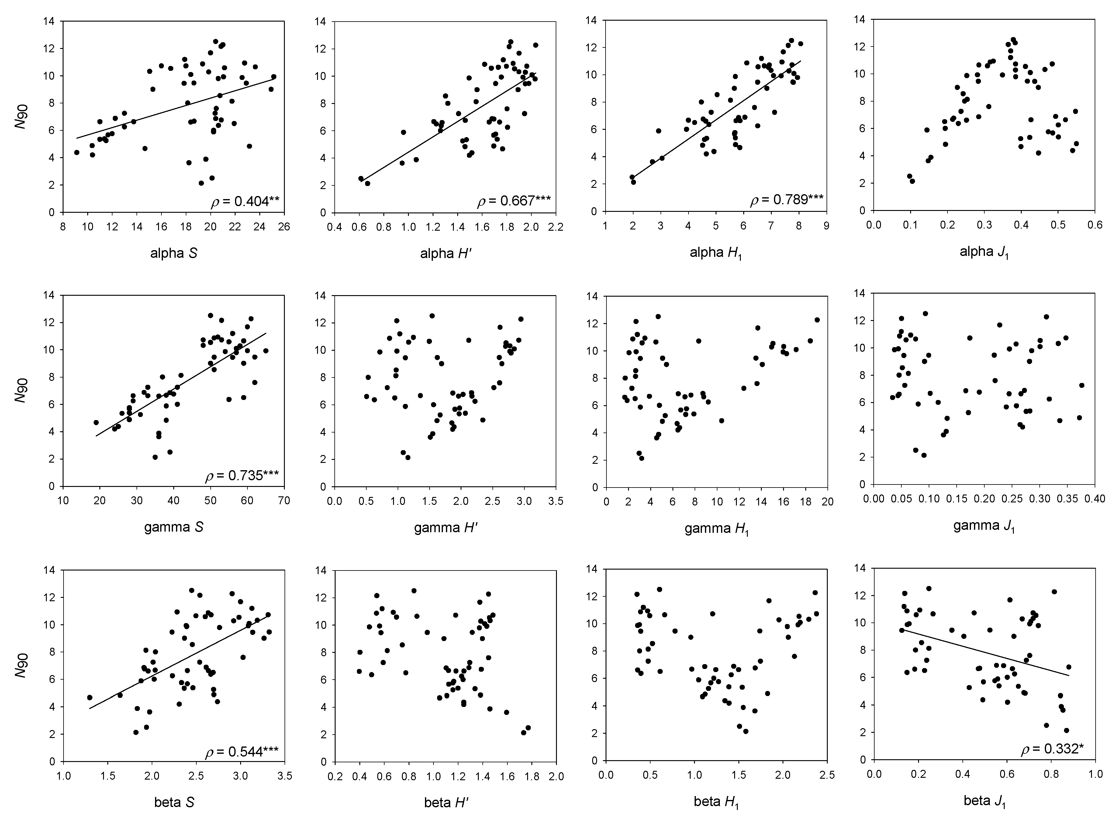
It is seen from the results for all strata and years that the highest correlations with N90 are related to the gamma version of S (ρ = 0.735; Figure 3) and the alpha version of H1 (ρ = 0.789; Figure 3) and H′ (ρ = 0.667; Figure 3). N90 also showed a positive correlation with beta S (ρ = 0.544; Figure 3).
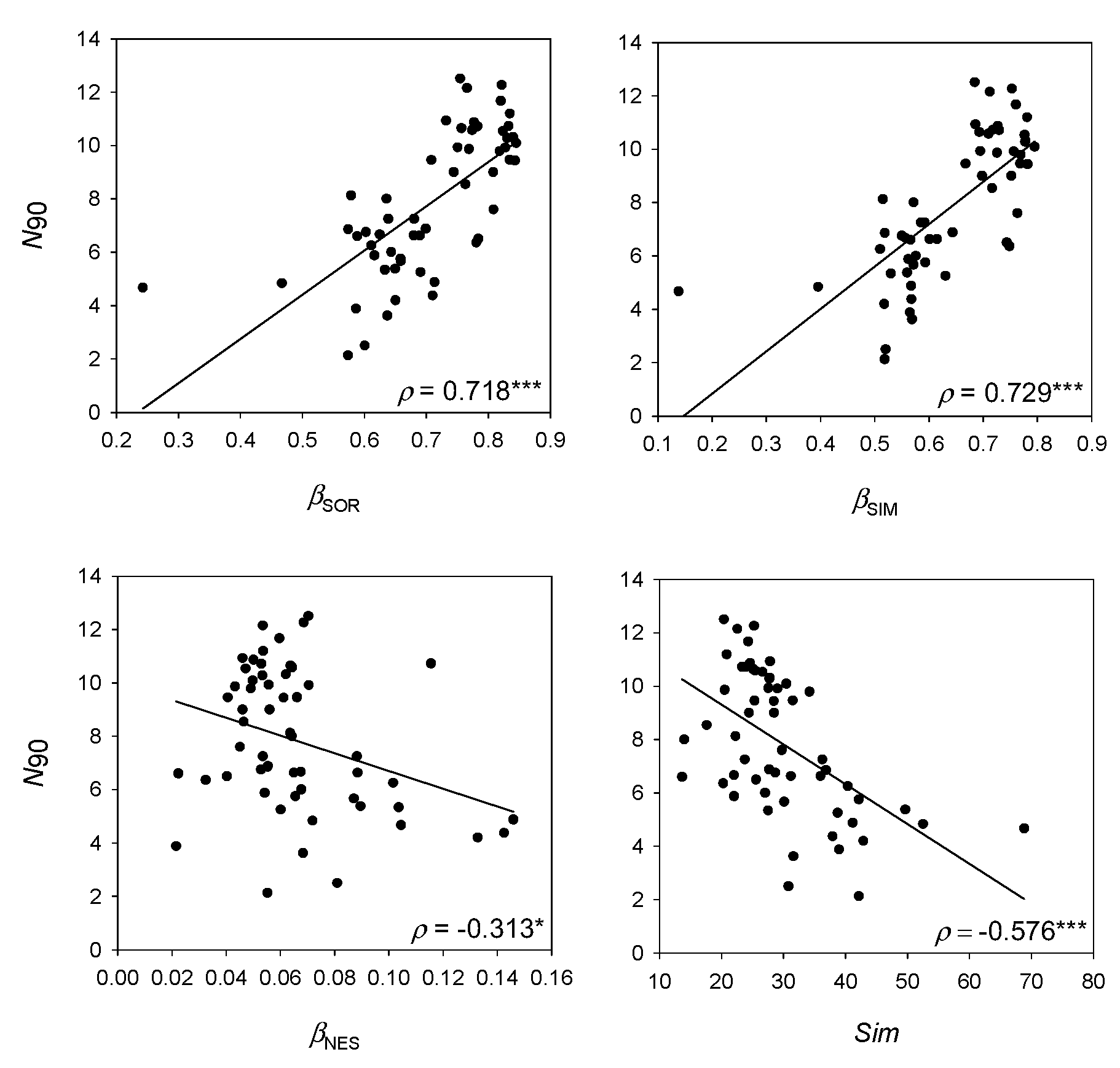
N90 showed a positive correlation with (ρ = 0.718; Figure 4) and (ρ = 0.729; Figure 4), and a negative correlation with (ρ = −313; Figure 4) and Sim (ρ = −0.576; Figure 4).
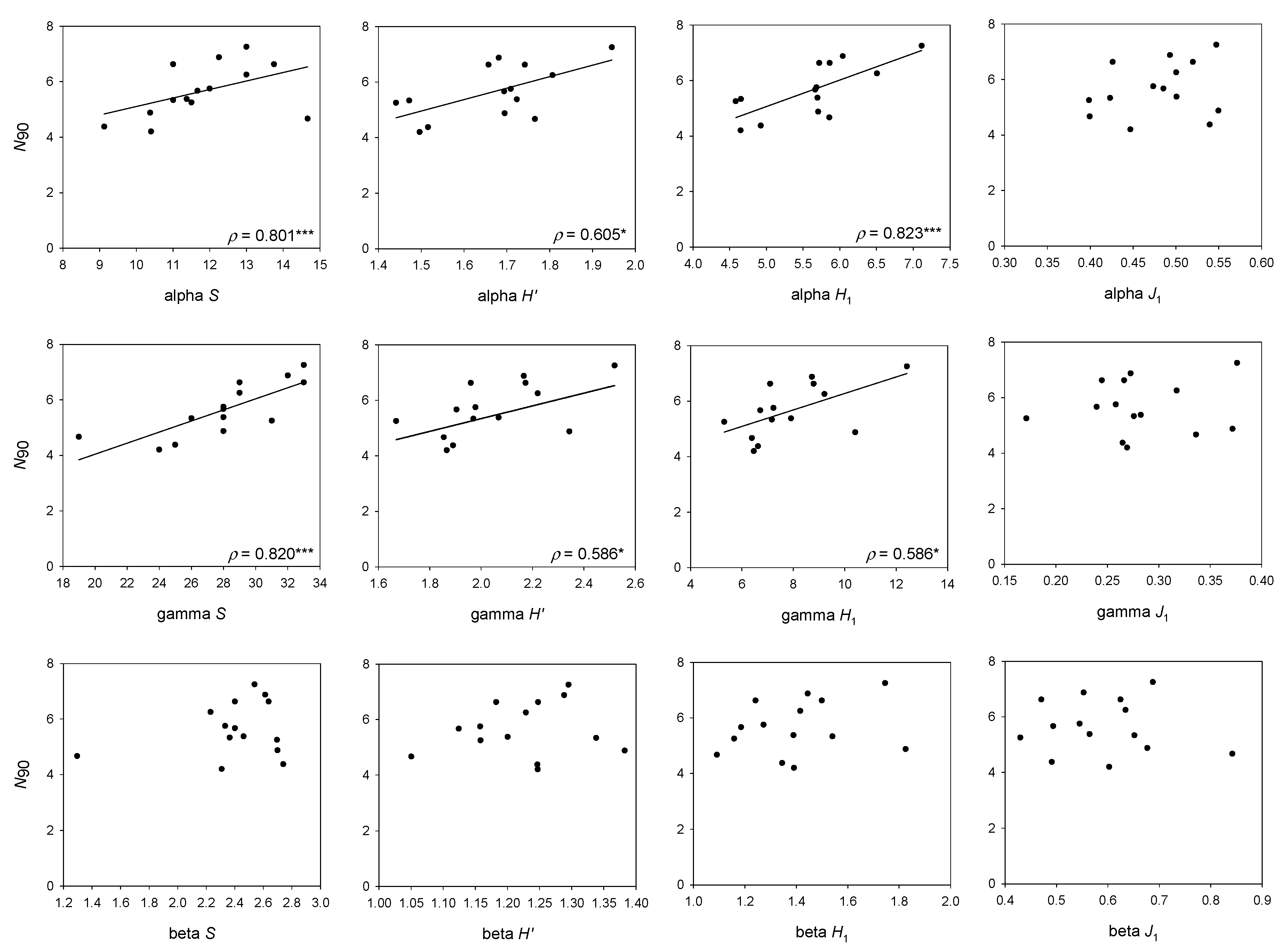
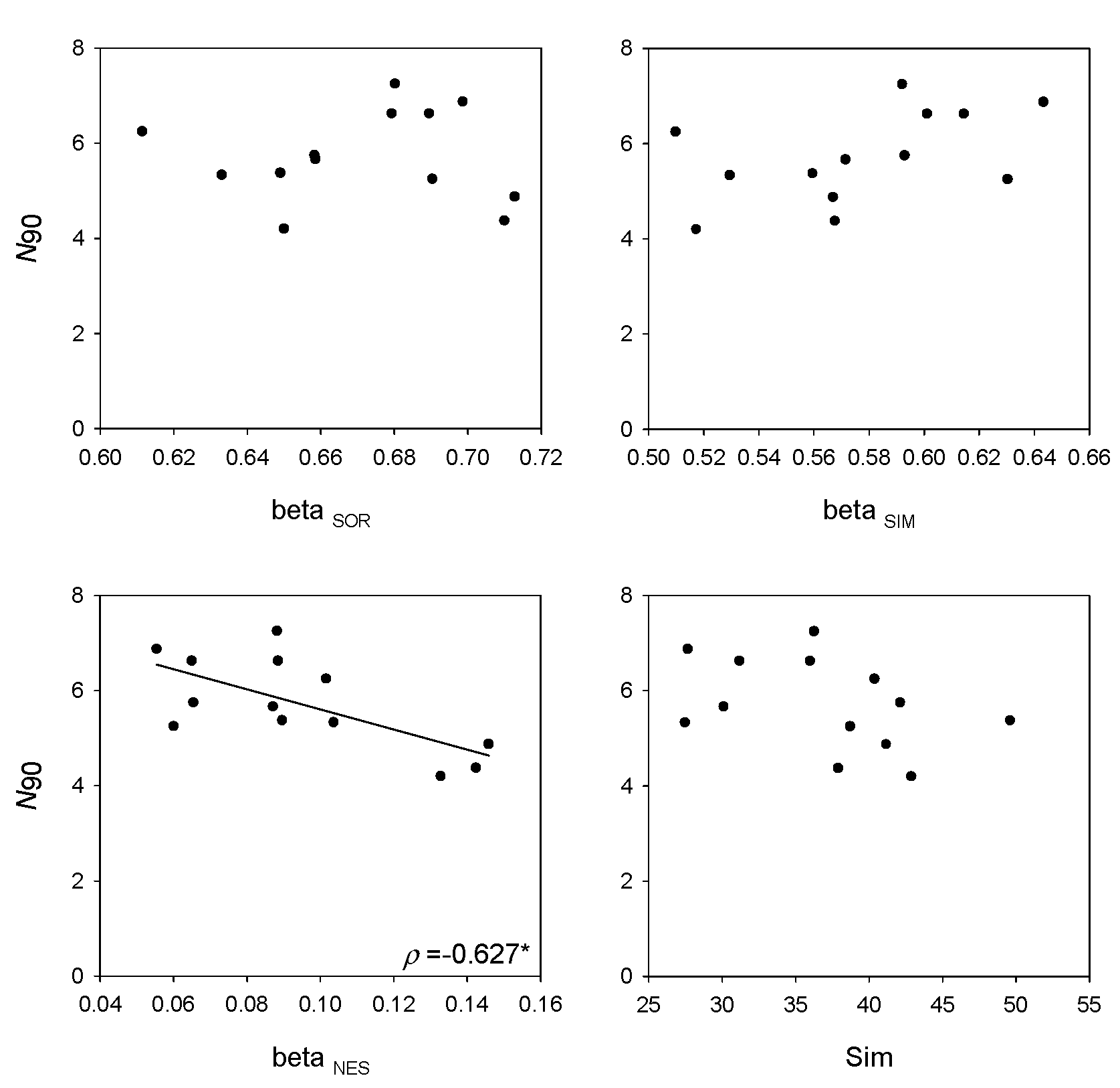
The stratum showing the highest values of nestedness was middle slope (501–800 m depth; βNES = 0.095). For this stratum, N90 showed a positive correlation with the gamma version of S (ρ = 0.820; Figure 5), H′ (ρ = 0.586; Figure 5) and H1 (ρ = 0.586; Figure 5), and the alpha version of S (ρ = 0.801; Figure 5), H1 (ρ = 0.823; Figure 5) and H′ (ρ = 0.605; Figure 5); and a negative correlation with βNES (ρ = −0.627; Figure 6).
4. Discussion
We have presented the N90 diversity index, which is based on the results of the SIMPER analysis and represents the number of species contributing up to ninety percent of within-group similarity in a group of samples. The hypothesis behind the index is that impacted communities may see both the frequency of occurrence and the evenness of the distribution of species abundances reduced among samples. This leads to a decrease in N90 due to the retreat of species populations to the localities presenting the most favorable ecological conditions. The N90 diversity index has the following advantages when compared to other diversity indices: (i) easy interpretation—units are number of species as in species richness (S), but, at the same time, the high dependence on sample size of S [23,24,25] is less important in N90, as rare species are not usually among the main contributors to within-group similarity; (ii) more sensitivity to anthropogenic impacts and environmental variability and their synergistic effects [13]; (iii) it assesses diversity for the whole set of samples in the group (usually representing a community or ecosystem) instead of operating at sample level and averaging values afterwards, or alternatively, pooling data from different samples (e.g., an S value taking into account all species appearing in all samples); and (iv) species identity is preserved because the N90 index is accompanied by a SIMPER table showing within-group species contribution to the 90% similarity. Finally, thanks to the re-sampling routine implemented in the calculation of N90, the index has a dispersion value associated that allows the comparison of values between areas or different periods.
The application of the N90 index to a non-real data set has enabled us to see the variation of the index to controlled changes in abundance distribution and number of species between samples in several groups and compare it to a battery of values of other indices. As expected, when abundances of all species are equal, a higher value of N90 is reached when these abundances are equally distributed among samples. And like all the other indices, N90 do not change when the abundance of all species in all samples changes equally. The main cause of decreases in N90 under these limited conditions is the disappearance of species in the group (decreases in gamma S). In that sense, the null contribution of absent species to Bray–Curtis similarity, and therefore to N90, is another advantage of the index, to avoid the consideration of those communities that do not share any species as being similar [15]. N90 is also sensitive to abundance evenness at the gamma level, reflected in decreases in the index in groups with identical samples (i.e., maximum similarity) but lower gamma H′, H1 and J’. The detection of changes in abundance distribution of species between samples is important in the detection of diversity loss due to the fishing-induced retreatment of species populations to localities presenting the most favourable ecological conditions. For that reason, it is important that N90 is based on a measure of similarity between samples influenced by the evenness of abundance at the gamma level, like Bray–Curtis. Besides, the use of absolute abundance in the calculation of N90 is preferred to allow the index to capture these changes in abundance distributions. Although these calculations based on non-real data give an idea about the behavior of N90 under repeatable and controlled conditions, its application to a real data set allows the analysis of data under natural conditions, with more variations in values of abundance distributions among samples. Changes in N90 due to nestedness and turnover of species between samples are discussed below.
For the whole bathymetric range considered, the higher correlation of N90 with the effective form of alpha H′ shows that values of N90, whose calculation is based on the comparison of the abundances of each pair of samples composing the group or community, are more similar to a mean value of H1 in the samples of the group or the community (alpha H1) than H1 calculated for the whole community (gamma H1). This means that frequent species in the group or community contribute more to N90 than abundant species (i.e., with absolute abundant values) in the whole community. This is endorsed by the high correlation of N90 and total number of species in the whole group of samples or community (gamma S). The difference between alpha, beta and gamma S is that alpha S takes the mean number of species in the community, beta S the replacement of species between samples of the community and gamma S is the total number of species in the community. Thus, the high correlation of N90 with gamma S has an easy explanation, because the species identity is not lost and the total number of species in the community is taken into account during the calculation of N90. However, N90 is not equal to gamma S, because it only takes into account the species that contribute to 90% similarity in the group of samples—or in other words, the species that are more representative in terms of frequency of appearance and abundance from the group of samples in the community.
Having N90 at halfway between alpha H1 and gamma S (mean N90 was 7.8, mean gamma S was 44.3 and mean alpha H1 was 5.8, for the whole set of samples) may favor the detection of the reduction in total (gamma) S through reductions in the frequency of occurrence, and on mean (alpha) H1 through reductions in the evenness of the distribution of species abundances among samples in impacted communities. Altogether, this would allow the detection of the diversity loss due to fishing.
The positive correlation of N90 with beta S denotes that beta S would increase due to an increase in the total number of species (gamma S), not compensated for by an increase in mean S (alpha S). However, at least some of the species increasing gamma S, although not frequent enough to change the mean S, would be evenly distributed enough to contribute to the value of the N90, allowing this index to account for some portion of the beta diversity.
N90 showed higher correlation with the turnover component of beta diversity than with nestedness, meaning that species replacement between samples has a higher weight in the calculation of the index than species loss. Previous works aimed to detect changes in diversity due to fishing impacts have shown that N90 is influenced by both turnover and nestedness. On one hand, species loss was the main cause of decreases in N90 in trawled demersal fish communities [13,26,27]. On the other, changes in diversity of epibenthic communities due to trawling were detected through the replacement of some vulnerable species by others more adapted to fishing, hence not involving a decrease in N90 values between impacted and non-impacted areas [28]; in that sense, we could expect that nestedness would be more important component of N90 than turnover. However, considering the data analyzed includes a large bathymetric range (50–800 m depth), turnover seems more plausible than species loss because the main factor structuring the community in the study area, as in the rest of the Mediterranean (e.g., [27]), is depth and not fishing impact. In any case, and because both processes can influence the results of N90, it is important to emphasize that the identity of the species is not lost during its calculation and the associated SIMPER table with the species contribution to similarity permits the knowledge of which species contribute to N90 and if changes in N90 are due to loss or replacement of species in the community.
Within-group similarity can be seen as an inverse measure of beta diversity and is based on the Bray–Curtis similarity index, which includes abundance of species in the calculation. On the contrary, measures of turnover and nestedness are calculated from presence–absence data [7]. The lower correlation of N90 and within-group similarity compared to measures of nestedness and turnover reinforces the idea conceived from this work that the frequency of appearances of species has more weight in the calculation of N90 than the distribution of abundances between samples. However, the high correlation of N90 with beta diversity measures and the fact that it is an indexed measure whose calculation relies on a similarity index, lead to it being included in the group of beta diversity indices.
The application of the analysis to middle slope stratum deepens in the results obtained for the whole depth range. In this stratum the correlation of N90 with alpha and gamma S increases. Additionally, N90 shows a higher correlation with nestedness than with turnover components of beta diversity. The difference between the whole depth range analysis and middle slope is that in the last case, the same community is considered in different years, whereas several demersal fish communities are considered when we analyze the larger depth gradient (e.g., [26,27]). Altogether, this indicates that N90 reflects an increase in gamma S due to the replacement of species between different communities when the whole depth range is considered, reflected by an increase of N90. While in a particular stratum, i.e., within the same bathymetric assemblage where species turnover or replacement is lower between samples, species loss and differences in number of species are the main causes of change. However, and contrary to communities mainly influenced by turnover, the fact that nestedness can impact gamma H1, which in turn impacts N90, must also be considered. In any case, N90 provides different information depending on whether we analyze heterogeneous or homogenous communities, with communities in which more species show a more even spread of their abundance showing higher values of N90 at any gradient of change.
Again, the associated SIMPER results will allow us to elucidate the relative importance of nestedness and turnover components of beta diversity on N90, and hence, identify the effects of impacts on marine communities. This has been proved in previous works where SIMPER tables allowed the identification of species that disappeared from the community due to their vulnerability to fishing activities, like elasmobranchs, or to their state of exploitation, like some by-catch species of bottom trawl fishery in the Balearic Islands in areas subjected to a high level of bottom trawling [13]. It also allowed the identification of species replaced by smaller ones in a trawled area [28]. As such, the study of the ecology of species that contribute to N90 through the SIMPER table is relevant to determine if fishing has caused a change in diversity due to the loss of vulnerable species or replacement by those more adapted to fishing impacts. However, this advantage is also useful for general ecological studies, in order to detect which kind of species are structuring the community.
Up to now, the N90 index has contributed to the comparison and explanation of specific data pools of exploited marine ecosystems and their living resources; it has been applied in the Mediterranean to assess the impact of fishing exploitation on the diversity of demersal fish and epi-benthic communities, both at narrow and broad bathymetric and geographical scales and considering both continuous and stratified approaches regarding levels of fishing effort [13,26,27,28]. In all cases, N90 displayed a better response to fishing pressure compared to other diversity indices covering a wide variety of aspects like the number of species and their relative abundance, as well as their taxonomic and functional position [23,29,30,31,32,33] Table 3, showing lower values in impacted communities. N90 has also been applied to assess spatio-temporal variations of diversity in fishing waste from north-western Mediterranean bottom trawl fishery [34]. In that case, similar results were obtained for species richness, but N90 gave information not only about the number of species but also on the species composition of the waste.
Indicators, defined as variables, pointers or indices of a phenomenon, are needed to support the implementation of the Ecosystem Approach to Fisheries, as they can provide information on the state of the ecosystems by tracking those components and attributes that may be adversely impacted by fishing, like diversity [35]. For the above-mentioned reasons, the N90 index can be a useful indicator for this. In addition, N90 also detects fishing impacts by fluctuating in response to environmental variation [11], making this index sensitive to the synergies between climate and fishing impacts at the community level. The sensitivity of N90 to reductions in the frequency of occurrence and the evenness of the distribution of species abundances among samples in impacted communities, together with the identification of both effects of fishing impacts, species replacement and species loss [13,26,28], make the N90 diversity index an alternative to ‘traditional’ diversity indices when trying to monitor fishing impacts within the current context of global change. Additionally, the comparison of N90 with a battery of indices to explore its properties performed here will make it more useful to those who decide to use it.
Supplementary Materials
The following are available online at https://0-www-mdpi-com.brum.beds.ac.uk/article/10.3390/d13100489/s1, Non-real data set: ‘nonreal_sp.csv’ and ‘nonreal_group.csv’, R script to calculate N90: N90_script.R, Appendix A data set: Data_sp.csv and Data_group.csv.
Author Contributions
Conceptualization, M.T.F., F.O. and E.M.; Funding acquisition, E.M.; Methodology, M.T.F. and F.O.; Software, M.T.F.; Supervision, F.O. and E.M.; Writing—original draft, M.T.F.; Writing—review & editing, F.O. and E.M. All authors have read and agreed to the published version of the manuscript.
Funding
The MEDITS scientific surveys are funded by the European Union Data Collection Framework for the Common Fisheries Policy. M. Teresa Farriols was supported by a FPI Fellowship (BES-2013-065112), which was developed within ECLIPSAME (CTM2012-37701) and CLIFISH (CTM2015-66400-C3-1-R MINECO/FEDER). Both fellowship and projects were funded by the Spanish Ministry of Economy and Competitiveness. More recently this research has been funded and performed within the scope of the LIFE IP INTEMARES project, coordinated by the Biodiversity Foundation of the Ministry for the Ecological Transition and the Demographic Challenge and receiving the financial support from the European Union’s LIFE programme (LIFE15 IPE ES 012).
Institutional Review Board Statement
Ethical review and approval were waived for this study, due that real data have been obtained in the framework of the MEDITS research surveys, which follow a sampling scheme and standartized protocol approved by international authorities (EU/DG Mare, FAO/GFCM). If a live specimen of a rare species or a species subject to conservation measures was caught, it was quickly sampled (4–5 minutes) and returned back to the sea unharmed, giving it a chance for survival, following the recommendation GFCM/36/2012/3 (http://www.gfcmonline.org/decisions/) on fisheries management measures for conservation of sharks and rays in the GFCM area.
Data Availability Statement
No new data were created or analyzed in this study. Data sharing is not applicable to this article. In any case, the access to the MEDITS data base was formerly regulated by the EU Reg. 199/2008 (Data Collection Framework) and currently by the regulation (EU) 2017/1004 (recast).
Acknowledgments
The present study could not have been done without the work of all the participants and crew during the MEDITS scientific surveys. The authors thank Eduard Szöcs and Paz Sampedro very much for their help and guidance in developing the script, as well as the valuable comments of two anonymous referees that helped us to improve the manuscript.
Conflicts of Interest
The authors declare no conflict of interest.
Appendix A. N90 Script
Appendix A1. Data Sets
N90 was calculated using an R script, version 4.4.1 [16]. The data needed to work with the N90 script consists of two ‘.csv’ files. The first one includes the abundances of each species. In this data file, column labels are the species names and each row corresponds to a sample. The other file includes, in the same order as the previous one, a column named Group, indicating the group to which each sample belongs. These data sets must be imported with the names af (i.e., abundance file) and gf (i.e., groups file). The structure of af and gf is shown in Table A1. The Vegan package [17] is required to carry out all the analyses.
As an example, we have applied the N90 script functions to a non-real data set (‘Data_group.csv’ and ‘Data_sp.csv’ files). Table A1 shows the abundances of 13 species (A, B, C, D, E, F, G, H, I, J, K, L, and M) in 2 unique groups of samples named gA and gB. The data must be imported with the names af and gf from 2 ‘.csv’ files.

Table A1.
Abundance data by species and sample for each Group of samples used in the example. The columns under af show the data included in the abundance file, whereas the column under gf shows the data included in the groups file. A, B, C, D, E, F, G, H, I, J, K, L and M are the names of the species.
| af | gf | ||||||||||||
|---|---|---|---|---|---|---|---|---|---|---|---|---|---|
| A | B | C | D | E | F | G | H | I | J | K | L | M | Group |
| 0 | 0 | 0 | 23 | 23 | 0 | 0 | 0 | 0 | 0 | 0 | 235 | 0 | gA |
| 0 | 0 | 0 | 0 | 0 | 0 | 0 | 0 | 0 | 148 | 0 | 49 | 0 | gA |
| 0 | 0 | 0 | 47 | 0 | 24 | 0 | 0 | 284 | 0 | 24 | 0 | 0 | gA |
| 0 | 0 | 0 | 22 | 0 | 0 | 22 | 0 | 66 | 0 | 66 | 22 | 0 | gA |
| 0 | 0 | 0 | 0 | 0 | 0 | 0 | 0 | 578 | 0 | 46 | 0 | 0 | gA |
| 415 | 0 | 0 | 0 | 0 | 0 | 0 | 0 | 394 | 0 | 0 | 109 | 0 | gA |
| 0 | 0 | 175 | 0 | 0 | 0 | 0 | 0 | 0 | 197 | 197 | 372 | 0 | gA |
| 0 | 0 | 0 | 215 | 0 | 0 | 0 | 0 | 882 | 0 | 473 | 0 | 1269 | gA |
| 41 | 0 | 20 | 41 | 0 | 0 | 20 | 0 | 569 | 203 | 996 | 41 | 0 | gA |
| 39 | 0 | 20 | 20 | 0 | 0 | 0 | 0 | 255 | 0 | 39 | 79 | 1336 | gA |
| 43 | 0 | 43 | 299 | 0 | 0 | 0 | 0 | 2542 | 0 | 2392 | 0 | 0 | gB |
| 22 | 0 | 0 | 90 | 0 | 112 | 0 | 0 | 4969 | 0 | 627 | 0 | 67 | gB |
| 0 | 0 | 0 | 172 | 0 | 0 | 0 | 0 | 6919 | 0 | 57 | 0 | 96 | gB |
| 0 | 0 | 0 | 169 | 0 | 0 | 19 | 0 | 226 | 0 | 414 | 19 | 0 | gB |
| 0 | 21 | 21 | 63 | 126 | 0 | 0 | 0 | 0 | 0 | 820 | 147 | 84 | gB |
| 19 | 0 | 0 | 58 | 0 | 0 | 0 | 0 | 1451 | 0 | 0 | 19 | 0 | gB |
| 0 | 0 | 81 | 0 | 0 | 0 | 61 | 0 | 0 | 606 | 20 | 323 | 0 | gB |
| 0 | 0 | 0 | 74 | 0 | 18 | 0 | 0 | 129 | 18 | 147 | 0 | 0 | gB |
| 38 | 0 | 19 | 208 | 0 | 0 | 0 | 0 | 5179 | 0 | 151 | 0 | 1115 | gB |
| 72 | 0 | 0 | 192 | 0 | 0 | 0 | 48 | 3006 | 0 | 577 | 0 | 24 | gB |
| 56 | 0 | 37 | 111 | 0 | 0 | 0 | 37 | 130 | 19 | 167 | 93 | 501 | gB |
| 0 | 0 | 37 | 130 | 0 | 0 | 0 | 0 | 5329 | 0 | 3182 | 0 | 0 | gB |
| 18 | 0 | 165 | 202 | 0 | 0 | 0 | 0 | 3813 | 0 | 1540 | 0 | 1228 | gB |
| 55 | 0 | 92 | 18 | 0 | 0 | 18 | 0 | 4055 | 110 | 1468 | 0 | 18 | gB |
| 0 | 0 | 538 | 0 | 0 | 0 | 36 | 0 | 18 | 341 | 72 | 269 | 18 | gB |
| 0 | 0 | 805 | 98 | 39 | 0 | 0 | 0 | 20 | 393 | 1374 | 569 | 2061 | gB |
| 273 | 0 | 243 | 273 | 0 | 0 | 30 | 0 | 1031 | 0 | 576 | 121 | 909 | gB |
| 60 | 0 | 0 | 80 | 0 | 0 | 20 | 40 | 40 | 60 | 498 | 179 | 0 | gB |
| 19 | 0 | 0 | 93 | 0 | 0 | 0 | 75 | 1325 | 0 | 523 | 0 | 0 | gB |
| 19 | 0 | 0 | 19 | 0 | 0 | 0 | 0 | 8519 | 0 | 167 | 0 | 1318 | gB |
| 18 | 0 | 0 | 0 | 0 | 0 | 18 | 0 | 733 | 0 | 72 | 0 | 0 | gB |
| 0 | 0 | 0 | 0 | 0 | 0 | 0 | 0 | 0 | 425 | 0 | 58 | 0 | gB |
| 0 | 0 | 0 | 0 | 38 | 0 | 19 | 0 | 0 | 0 | 303 | 114 | 132 | gB |
| 0 | 0 | 0 | 37 | 0 | 0 | 0 | 18 | 3118 | 0 | 1339 | 0 | 18 | gB |
| 0 | 0 | 0 | 59 | 0 | 0 | 0 | 59 | 2121 | 0 | 238 | 0 | 1407 | gB |
| 21 | 0 | 0 | 21 | 0 | 0 | 0 | 0 | 2987 | 0 | 165 | 0 | 0 | gB |
| 0 | 0 | 370 | 0 | 0 | 0 | 0 | 0 | 0 | 206 | 62 | 637 | 0 | gB |
| 0 | 0 | 40 | 20 | 20 | 0 | 0 | 0 | 0 | 0 | 418 | 358 | 219 | gB |
| 0 | 0 | 20 | 40 | 0 | 0 | 0 | 81 | 161 | 20 | 1732 | 624 | 20 | gB |
| 24 | 0 | 235 | 400 | 0 | 0 | 0 | 71 | 3695 | 0 | 1695 | 47 | 4590 | gB |
Appendix A2. Exploring Data
The Data_explore (af, gf, perc, perc2) function allows the exploration of the data prior to application of the jack-knife re-sampling routine. For each Group given in gf it returns: (1) the number of samples in each group (n); (2) the number of samples that will be removed in each re-sampling (n1) for a specified percentage of samples to be removed (perc; if perc accounts for less than one sample, the function will consider n1 = 1 by default); and (3) the maximum number of samples in n1 that can be repeated in the next re-sampling for a specified percentage perc2. Both perc and perc2 are implemented as integer divisions in the script. This function allows users to explore the samples replaced in each jack-knife using different values of perc and perc2.
We applied the Data_explore (af, gf, perc = 10, perc2 = 70) function, in which 10 percent of samples were removed in each re-sampling (perc), and 70 percent of removed samples were repeated from the previous resampling (perc2) to the non-real data set in Section 1.
For our example data set the output was:
Group: “1”
Name of the group: “gA”
Number of samples of the group: “10”
Number of samples removed: “1”
Maximum number of repeated samples from removed: “0”
Group: “2”
Name of the group: “gB”
Number of samples of the group: “30”
Number of samples removed: “3”
Maximum number of repeated samples from removed: “2”
This shows that in the first group (gA) there are 10 samples and that the number of samples removed in each re-sampling with the given percentage (perc = 10) is n1 = 1, of which none should be repeated according to the given perc2 (perc2 = 70). In the second group (gB) there are 30 samples; the number of samples removed in each re-sampling with the given percentage (perc = 10) is n1 = 3. The number of samples that should can be repeated according perc2 (perc2 = 70) is 2.
Appendix A3. Resampling N90
The N90_resampling (af, gf, cutoff = 90, perc, perc2, jkmax) function executes the jack-knife re-sampling routine and returns the value of the N90 index. With the value of jkmax, the user can specify the number of re-samples to be done. The maximum value of jkmax permitted for the script is 9999. If this value is overtaken, the function will return a ‘WARNING’ message. The argument cutoff allows specification of a different cutoff percentage of accumulated species contribution to within-group similarity than the 90% used by default in the N90 index (i.e., cutoff = y then Ny). The use of the arguments perc and perc2 has been already explained for the Data_explore (af, gf, perc, perc2) function in Section 2.
At the end of the calculation, the N90_resampling (af, gf, cutoff = 90, perc, perc2, jkmax) function returns a list with 3 objects. The $N90_jackknifes object reports the value of the n90 index (n90.jackknife) and the within-group similarity (Sim.jackknife) obtained in each re-sampling for each Group given in gf. The $N90_mean_values object reports the mean value of the N90 index (Av.N90) and its standard deviation (SD.N90), and the mean within-group similarity (Av.Sim) and its standard deviation (SD.Sim), both calculated taking into account all the values obtained in each re-sampling for each Group given in gf. And finally, the $SIMPER_table object includes a SIMPER table for each Group given in gf that shows the contribution of all the species included in the group of samples. These SIMPER tables are generated taking into account all the samples (i.e., without re-sampling). For each Species in a Group the table shows: the mean abundance (Av.Abund) and its standard deviation (SD.Abund), the mean contribution (Av.Si) and its standard deviation (SD.Si) to within-group similarity, the percentage contribution to within-group similarity (Contr), and the cumulative contribution to within-group similarity (Cum).
For the present example, N90_resampling (af, gf, cutoff = 90, perc = 10, perc2 = 70, jkmax = 9999), the perc = 10 and the perc2 = 70 previously explored in Section 2, are used. The output list (named as my_list in N90 script) consists of 3 objects: The $N90_jackknifes object summarizing the results of the n90 value and the mean within-group similarity in each re-sampling (Table A2); the $N90_mean_values object summarizing the N90 value and the mean within-group similarity, with their standard deviations for all groups in gf (Table A3); finally, the $SIMPER_table object summarizing the SIMPER analysis results for each group of samples (Table A4). This table will allow identification of the species accounting for the N90 value due to their being ordered by their contribution to within-group similarity.
Table A2.
Jack-knife results table obtained using the N90_resampling function for group A (gA) from the $N90_jackknifes object. n90_jackknife and Sim_jackknife are the values of the n90 and the total similarity values in each re-sampling step, respectively.
Table A2.
Jack-knife results table obtained using the N90_resampling function for group A (gA) from the $N90_jackknifes object. n90_jackknife and Sim_jackknife are the values of the n90 and the total similarity values in each re-sampling step, respectively.
| Group | n90_jackknife | Sim_jackknife |
|---|---|---|
| gA | 5 | 23.727 |
| gA | 4 | 24.326 |
| gA | 5 | 20.527 |
| gA | 5 | 22.314 |
| gA | 5 | 19.980 |
| gA | 5 | 20.616 |
| gA | 4 | 22.541 |
| gA | 4 | 21.070 |
| gA | 4 | 20.011 |
| gA | 4 | 21.217 |
Table A3.
Average results table obtained using the N90_resampling function from the $N90_mean values object. Av.N90 and the SD.N90 are the N90 value and its standard deviation, respectively; Av.Sim and SD.Sim are the average and standard deviation values of the within-group similarity.
Table A3.
Average results table obtained using the N90_resampling function from the $N90_mean values object. Av.N90 and the SD.N90 are the N90 value and its standard deviation, respectively; Av.Sim and SD.Sim are the average and standard deviation values of the within-group similarity.
| Group | Av.N90 | SD.N90 | Av.Sim | SD.Sim |
|---|---|---|---|---|
| gA | 4.5 | 0.527 | 21.633 | 1.529 |
| gB | 4.395 | 0.490 | 29.631 | 1.201 |
Table A4.
SIMPER table obtained using the N90_resampling function from the $SIMPER_table object. Av.Abund and SD.Abund are the average and standard deviation values of the abundance, respectively; Av.Si and SD.Si are the mean and standard deviation of the contribution of each species to the within-group similarity; Contr is the percentage contribution to within-group similarity; and Cum is the cumulative percentage contribution.
| Group | Species | Av.Abund | SD.Abund | Av.Si | SD.Si | Contr | Cum |
|---|---|---|---|---|---|---|---|
| gA | I | 302.8 | 302.612 | 11.120 | 15.557 | 51.403 | 51.403 |
| gA | L | 90.7 | 122.035 | 3.964 | 7.167 | 18.325 | 69.727 |
| gA | K | 184.1 | 320.450 | 2.795 | 4.442 | 12.919 | 82.646 |
| gA | M | 260.5 | 549.409 | 1.219 | 8.177 | 5.635 | 88.281 |
| gA | J | 54.8 | 89.375 | 1.192 | 4.754 | 5.510 | 93.791 |
| gA | D | 36.8 | 64.966 | 1.039 | 2.092 | 4.805 | 98.596 |
| gA | A | 49.5 | 129.497 | 0.175 | 0.668 | 0.807 | 99.403 |
| gA | C | 21.5 | 54.572 | 0.087 | 0.334 | 0.404 | 99.807 |
| gA | G | 4.2 | 8.867 | 0.042 | 0.280 | 0.193 | 100 |
| gB | I | 2050.533 | 2371.281 | 14.989 | 21.685 | 50.584 | 50.584 |
| gB | K | 693.2 | 796.607 | 8.342 | 9.584 | 28.153 | 78.737 |
| gB | L | 119.233 | 194.182 | 1.769 | 4.734 | 5.970 | 84.708 |
| gB | M | 460.833 | 957.334 | 1.665 | 4.667 | 5.618 | 90.326 |
| gB | D | 97.533 | 101.775 | 1.265 | 1.801 | 4.269 | 94.594 |
| gB | J | 73.267 | 157.214 | 0.687 | 3.979 | 2.318 | 96.912 |
| gB | C | 91.533 | 184.478 | 0.522 | 1.992 | 1.763 | 98.675 |
| gB | A | 25.233 | 51.494 | 0.182 | 0.470 | 0.613 | 99.288 |
| gB | G | 7.367 | 14.454 | 0.096 | 0.414 | 0.323 | 99.611 |
| gB | H | 14.3 | 26.373 | 0.088 | 0.398 | 0.298 | 99.909 |
| gB | E | 7.433 | 24.624 | 0.026 | 0.253 | 0.087 | 99.996 |
| gB | F | 4.333 | 20.599 | 0.001 | 0.028 | 0.004 | 100 |
References
- Magurran, A.E. Measuring Biological Diversity; Blackwell Science Ltd.: Oxford, UK, 2004. [Google Scholar]
- Chao, A.; Chiu, C.H.; Hsieh, T.C. Proposing a resolution to debates on diversity partitioning. Ecology 2012, 93, 2037–2051. [Google Scholar] [CrossRef] [PubMed] [Green Version]
- Chao, A.; Gotelli, N.J.; Hsieh, T.C.; Sander, E.L.; Ma, K.H.; Colwell, R.K.; Ellison, A.M. Rarefaction and extrapolation with Hill numbers: A framework for sampling and estimation in species diversity studies. Ecol. Monogr. 2014, 84, 45–67. [Google Scholar] [CrossRef] [Green Version]
- Jost, L. Partitioning diversity into independent alpha and beta components. Ecology 2007, 88, 2427–2439. [Google Scholar] [CrossRef] [PubMed] [Green Version]
- Jurasinski, G.; Retzer, V.; Beierkuhnlein, C. Inventory, differentiation, and proportional diversity: A consistent terminology for quantifying species diversity. Oecologia 2009, 159, 15–26. [Google Scholar] [CrossRef] [PubMed] [Green Version]
- Tuomisto, H. A consistent terminology for quantifying species diversity? Yes, it does exist. Oecologia 2010, 164, 853–860. [Google Scholar] [CrossRef]
- Baselga, A. Partitioning the turnover and nestedness components of beta diversity. Glob. Ecol. Biogeogr. 2010, 19, 134–143. [Google Scholar] [CrossRef]
- Whittaker, R.H. Vegetation of the Siskiyou mountains, Oregon and California. Ecol. Monogr. 1960, 30, 279–338. [Google Scholar] [CrossRef]
- Whittaker, R.H. Evolution and measurement of species diversity. Taxon 1972, 12, 213–251. [Google Scholar] [CrossRef] [Green Version]
- Chao, A.; Chiu, C.H. Bridging the variance and diversity decomposition approaches to beta diversity via similarity and differentiation measures. Methods Ecol. Evol. 2016, 7, 919–928. [Google Scholar] [CrossRef]
- Legendre, P.; Borcard, D.; Peres-Neto, P.R. Analysing beta diversity: Partitioning the spatial variation and community composition data. Ecol. Monogr. 2005, 75, 435–450. [Google Scholar] [CrossRef]
- Anderson, M.J.; Ellingsen, K.E.; McArdle, B.H. Multivariate dispersion as a measure of beta diversity. Ecol. Lett. 2006, 9, 683–693. [Google Scholar] [CrossRef]
- Farriols, M.T.; Ordines, F.; Hidalgo, M.; Guijarro, B.; Massutí, E. N90 index: A new approach to biodiversity based on similarity and sensitive to direct and indirect fishing impact. Ecol. Indic. 2015, 52, 245–255. [Google Scholar] [CrossRef]
- Clarke, K.R. Non-parametric multivariate analyses of changes in community structure. Aust. J. Ecol. 1993, 18, 117–143. [Google Scholar] [CrossRef]
- Bray, J.R.; Curtis, J.T. An ordination of the upland forest communities of southern Wisconsin. Ecol. Monogr. 1957, 27, 325–349. [Google Scholar] [CrossRef]
- R Core Team. R: A Language and Environment for Statistical Computing. Available online: http://www.r-project.org/ (accessed on 20 September 2021).
- Oksanen, J.; Blanchet, F.G.; Kindt, R.; Legendre, P.; Minchin, P.R.; O’Hara, R.B.; Simpson, G.L.; Solymos, P.; Stevens, M.H.H.; Wagner, H. Vegan: Community Ecology Package. Available online: https://CRAN.R-project.org/package=vegan (accessed on 20 September 2021).
- Sørensen, T.A. A method of establishing groups of equal amplitude in plant sociology based on similarity of species content, and its application to analyses of the vegetation on Danish commons. K. Dan. Vidensk. Selsk. Biol. Skr. 1948, 5, 1–34. [Google Scholar]
- Koleff, P.; Gaston, K.J.; Lennon, J.K. Measuring beta diversity for presence–absence data. J. Anim. Ecol. 2003, 72, 367–382. [Google Scholar] [CrossRef] [Green Version]
- Simpson, G.G. Mammals and the nature of continents. Am. J. Sci. 1943, 241, 1–31. [Google Scholar] [CrossRef]
- Lennon, J.J.; Koleff, P.; Greenwood, J.J.D.; Gaston, K.J. The geographical structure of British bird distributions: Diversity, spatial turnover and scale. J. Anim. Ecol. 2001, 70, 966–979. [Google Scholar] [CrossRef] [Green Version]
- Spedicato, M.T.; Massutí, E.; Mérigot, B.; Tserpes, G.; Jadaud, A.; Relini, G. The MEDITS trawl survey specifications in an ecosystem approach to fishery management. Sci. Mar. 2019, 83, 9–20. [Google Scholar] [CrossRef]
- Hill, M.O. Diversity and evenness: A unifying notation and its consequences. Ecology 1973, 54, 427–432. [Google Scholar] [CrossRef] [Green Version]
- Noss, R.F. Indicators for monitoring biodiversity: A hierarchical approach. Conserv. Biol. 1990, 4, 355–364. [Google Scholar] [CrossRef]
- Gotelli, N.J.; Chao, A. Measuring and estimating species richness, species diversity, and biotic similarity from sampling data. In Encyclopedia of Biodiversity; Levin, S.A., Ed.; Academic Press: Waltham, MA, USA, 2013; pp. 195–211. [Google Scholar]
- Farriols, M.T.; Ordines, F.; Somerfield, P.J.; Pasqual, C.; Hidalgo, M.; Guijarro, B.; Massutí, E. Bottom trawl impacts on Mediterranean demersal fish diversity: Not so obvious or are we too late? Cont. Shelf Res. 2017, 137, 84–102. [Google Scholar] [CrossRef] [Green Version]
- Farriols, M.T.; Ordines, F.; Carbonara, P.; Casciaro, L.; Di Lorenzo, M.; Esteban, A.; Follesa, C.; García-Ruiz, C.; Isajlovic, I.; Jadaud, A.; et al. Spatio-temporal trends in diversity of demersal fish assemblages in the mediterranean. Sci. Mar. 2019, 83, 189–206. [Google Scholar] [CrossRef]
- Ordines, F.; Ramón, M.; Rivera, J.; Rodríguez-Prieto, C.; Farriols, M.T.; Guijarro, B.; Pasqual, C.; Massutí, E. Why long term trawled red algae beds off Balearic Islands (western Mediterranean) still persist? Reg. Stud. Mar. Sci. 2017, 15, 39–49. [Google Scholar] [CrossRef]
- Shannon, C.E.; Weaver, W. The Mathematical Theory of Communication; University of Illinois Press: Urbana, IL, USA, 1949. [Google Scholar]
- Margalef, R. Information theory in ecology. Gen. Syst. 1958, 3, 36–71. [Google Scholar]
- Pielou, E.C. Species-diversity and pattern-diversity in the study of ecological succession. J. Theor. Biol. 1966, 10, 370–383. [Google Scholar] [CrossRef]
- Warwick, R.M.; Clarke, K.R. New ‘biodiversity’ measures reveal a decrease in taxonomic distinctness with increasing stress. Mar. Ecol. Prog. Ser. 1995, 129, 301–305. [Google Scholar] [CrossRef] [Green Version]
- Somerfield, P.J.; Clarke, K.R.; Warwick, R.M.; Dulvy, N.K. Average functional distinctness as a measure of the composition of assemblages. ICES J. Mar. Sci. 2008, 65, 1462–1468. [Google Scholar] [CrossRef]
- Gorelli, G.; Blanco, M.; Sardà, F.; Carretón, M.; Company, J.B. Spatio-temporal variability of discards in the fishery of the deep-sea red shrimp Aristeus antennatus in the northwestern Mediterranean Sea: Implications for management. Sci. Mar. 2016, 80, 79–88. [Google Scholar] [CrossRef] [Green Version]
- Jennings, S. Indicators to support an ecosystem approach to fisheries. Fish Fish. 2005, 6, 212–232. [Google Scholar] [CrossRef]
Figure 1.
Calculation of number of species contributing to 90% similarity from SIMPER analysis in a group with 5 samples (n90). SIMPER table associated with n90 is also presented, where A is the average abundance of each species in the group; Si is the contribution of each species to within-group similarity; %C is the percentage contribution of each species to within-group similarity; and Σ is the cumulative percentage contribution. Intra-group similarity for this example was Sim = 40.8.

Figure 2.
Jack-knifes for the calculation of N90 in a group with 5 samples. In each Jack-knife a single sample is removed from the group and the number of samples contributing up to 90% to within-group similarity (n90) and the total similarity of the group is calculated. N90 is the mean value of n90 obtained from all the re-samplings.

Figure 3.
Results of the linear regression analysis of N90 with alpha, beta and gamma versions of Species Richness (S), Shannon (H′), Hill number of order 1 (H1) and the derived evenness measure (J1), considering the whole bathymetric range (50–800 m depth). The results for alpha, beta and gamma versions of J’ are not plotted because they do not show any correlation with N90. Spearman’s rank correlation coefficient (ρ), and p-values are presented. (*) p < 0.05; (**) p < 0.01; (***) p < 0.001.

Figure 4.
Results of the linear regressions analysis of N90 with measures of beta diversity βSOR, βSIM and βNES and within-group similarity (Sim), considering the whole bathymetric range (50–800 m depth). Spearman’s rank correlation coefficient (ρ) and p-values are presented. (*) p < 0.05; (**) p < 0.01; (***) p < 0.001.

Figure 5.
Results of the linear regression analysis of N90 with alpha, beta and gamma versions of Species Richness (S), Shannon (H′), Hill number of order 1 (H1) and the derived evenness measure (J1), considering the middle slope stratum (501–800 m depth). The results for alpha, beta and gamma versions of J’ are not plotted because they do not show any correlation with N90. Spearman’s rank correlation coefficient (ρ) and p-values are presented. (*) p < 0.05; (**) p < 0.01; (***) p < 0.001.

Figure 6.
Results of the linear regressions analysis of N90 with measures of beta diversity βSOR, βSIM and βNES and within-group similarity (Sim) considering the middle slope stratum (501–800 m depth). Spearman’s rank correlation coefficient (ρ) and p-values are presented. (*) p < 0.05; (**) p < 0.01; (***) p < 0.001.

Table 1.
Results of N90 and alpha, beta and gamma versions of Species Richness (S), Shannon (H′), Hill number of order 1 (H1) and Pielou’s evenness (J′) for the non-real data set. A is the mean abundance in the group of samples.
Table 1.
Results of N90 and alpha, beta and gamma versions of Species Richness (S), Shannon (H′), Hill number of order 1 (H1) and Pielou’s evenness (J′) for the non-real data set. A is the mean abundance in the group of samples.
| Alpha | Gamma | Beta | |||||||||||||||
|---|---|---|---|---|---|---|---|---|---|---|---|---|---|---|---|---|---|
| Group | A | N90 | S | H′ | H1 | J′ | J1 | S | H′ | H1 | J′ | J1 | S | H′ | H1 | J′ | J1 |
| A | 200 | 18 | 20 | 3.00 | 20.00 | 1.00 | 1.00 | 20.00 | 3.00 | 20.00 | 1.00 | 1.00 | 1.00 | 1.00 | 1.00 | 1.00 | 1.00 |
| B | 100 | 18 | 20 | 3.00 | 20.00 | 1.00 | 1.00 | 20.00 | 3.00 | 20.00 | 1.00 | 1.00 | 1.00 | 1.00 | 1.00 | 1.00 | 1.00 |
| C | 150 | 17 | 20 | 2.94 | 18.90 | 0.98 | 0.95 | 20.00 | 2.94 | 18.90 | 0.98 | 0.95 | 1.00 | 1.00 | 1.00 | 1.00 | 1.00 |
| D | 100 | 9 | 10 | 2.30 | 10.00 | 1.00 | 1.00 | 10.00 | 2.30 | 10.00 | 1.00 | 1.00 | 1.00 | 1.00 | 1.00 | 1.00 | 1.00 |
| E | 150 | 18 | 20 | 3.00 | 20.00 | 1.00 | 1.00 | 20.00 | 3.00 | 20.00 | 1.00 | 1.00 | 1.00 | 1.00 | 1.00 | 1.00 | 1.00 |
| F | 125 | 13 | 15 | 2.66 | 14.36 | 0.98 | 0.96 | 15.00 | 2.66 | 14.36 | 0.98 | 0.96 | 1.00 | 1.00 | 1.00 | 1.00 | 1.00 |
| G | 110 | 10 | 11 | 2.20 | 11.00 | 1.00 | 1.00 | 20.00 | 2.84 | 17.19 | 0.95 | 0.86 | 1.82 | 1.29 | 1.56 | 0.95 | 0.86 |
| H | 155 | 13.2 | 15.5 | 2.72 | 15.50 | 1.00 | 1.00 | 20.00 | 2.90 | 18.16 | 0.97 | 0.91 | 1.29 | 1.06 | 1.17 | 0.97 | 0.91 |
| I | 100 | 14.4 | 10 | 2.22 | 10.00 | 1.00 | 1.00 | 20.00 | 2.95 | 19.10 | 0.98 | 0.96 | 2.00 | 1.33 | 1.91 | 0.98 | 0.96 |
| J | 112 | 14.6 | 11.2 | 2.38 | 11.20 | 1.00 | 1.00 | 20.00 | 2.95 | 19.01 | 0.98 | 0.95 | 1.79 | 1.24 | 1.70 | 0.98 | 0.95 |
| K | 62.5 | 14.4 | 11.2 | 2.35 | 10.90 | 0.99 | 0.97 | 20.00 | 2.93 | 18.76 | 0.98 | 0.94 | 1.79 | 1.25 | 1.72 | 0.99 | 0.96 |
| L | 127 | 13.4 | 12.7 | 2.44 | 12.70 | 1.00 | 1.00 | 20.00 | 2.94 | 18.88 | 0.98 | 0.94 | 1.57 | 1.20 | 1.49 | 0.98 | 0.95 |
Table 2.
Results of N90 and values of βSOR, βSIM, βNES and within-group similarity (Sim) for the non-real data set. A is the mean abundance in the group of samples.
Table 2.
Results of N90 and values of βSOR, βSIM, βNES and within-group similarity (Sim) for the non-real data set. A is the mean abundance in the group of samples.
| Group | A | N90 | βSOR | βSIM | βNES | Sim |
|---|---|---|---|---|---|---|
| A | 200 | 18 | 0.00 | 0.00 | 0.00 | 100.00 |
| B | 100 | 18 | 0.00 | 0.00 | 0.00 | 100.00 |
| C | 150 | 17 | 0.00 | 0.00 | 0.00 | 100.00 |
| D | 100 | 9 | 0.00 | 0.00 | 0.00 | 100.00 |
| E | 150 | 18 | 0.00 | 0.00 | 0.00 | 81.48 |
| F | 125 | 13 | 0.00 | 0.00 | 0.00 | 100.00 |
| G | 110 | 10 | 0.65 | 0.00 | 0.65 | 63.12 |
| H | 155 | 13.2 | 0.38 | 0.00 | 0.38 | 88.05 |
| I | 100 | 14.4 | 0.74 | 0.61 | 0.12 | 47.55 |
| J | 112 | 14.6 | 0.70 | 0.59 | 0.10 | 56.50 |
| K | 62.5 | 14.4 | 0.70 | 0.59 | 0.10 | 51.81 |
| L | 127 | 13.4 | 0.64 | 0.32 | 0.31 | 63.38 |
Table 3.
Diversity indices which have been compared to the N90 in previous studies [23, 29,30,31,32,33].
| Index | Description | Reference |
|---|---|---|
| Species richness | Total number of species | |
| Shannon | Measure of uncertainty about the species of the nearest neighbour of an individual from the community | [29] |
| Margalef’s richness | Number of species adjusted to the number of individuals | [30] |
| Pielou’s evenness | Equitability in the distribution of abundances of species in a community | [31] |
| Reciprocal Berger–Parker | Inverse of the dominance of species | [23] |
| Taxonomic distinctness | Taxonomic distance expected between two individuals randomly selected, considering that they belong to different species | [32] |
| Functional diversity | Functional distance expected between two individuals randomly selected | [33] |
| Functional distinctness | Functional distance expected between two individuals randomly selected, considering that they belong to different species | [33] |
Publisher’s Note: MDPI stays neutral with regard to jurisdictional claims in published maps and institutional affiliations. |
© 2021 by the authors. Licensee MDPI, Basel, Switzerland. This article is an open access article distributed under the terms and conditions of the Creative Commons Attribution (CC BY) license (https://creativecommons.org/licenses/by/4.0/).
Share and Cite
MDPI and ACS Style
Farriols, M.T.; Ordines, F.; Massutí, E. N90, a Diversity Index Sensitive to Variations in Beta Diversity Components. Diversity 2021, 13, 489. https://0-doi-org.brum.beds.ac.uk/10.3390/d13100489
AMA Style
Farriols MT, Ordines F, Massutí E. N90, a Diversity Index Sensitive to Variations in Beta Diversity Components. Diversity. 2021; 13(10):489. https://0-doi-org.brum.beds.ac.uk/10.3390/d13100489
Chicago/Turabian StyleFarriols, M. Teresa, Francesc Ordines, and Enric Massutí. 2021. "N90, a Diversity Index Sensitive to Variations in Beta Diversity Components" Diversity 13, no. 10: 489. https://0-doi-org.brum.beds.ac.uk/10.3390/d13100489
Note that from the first issue of 2016, this journal uses article numbers instead of page numbers. See further details here.