Article

Comparing the Utility of Microsatellites and Single Nucleotide Polymorphisms in Conservation Genetics: Insights from a Study on Two Freshwater Fish Species in France

by
Jérôme G. Prunier
1,*,
Charlotte Veyssière
2,
Géraldine Loot
2 and
Simon Blanchet
1,2,*
1
Centre National de la Recherche Scientifique (CNRS), Université Paul Sabatier (UPS), Station d’Ecologie Théorique et Expérimentale, UAR 2029, F-09200 Moulis, France
2
CNRS, UPS, École Nationale de Formation Agronomique (ENFA), UMR 5174 EDB (Laboratoire Évolution & Diversité Biologique), 118 Route de Narbonne, CEDEX 4, F-31062 Toulouse, France
*
Authors to whom correspondence should be addressed.
Submission received: 3 April 2023 / Revised: 15 May 2023 / Accepted: 16 May 2023 / Published: 18 May 2023

Abstract

:
Biodiversity is facing an unprecedented crisis and substantial efforts are needed to conserve natural populations, especially in river ecosystems. The use of molecular tools to guide conservation practices in rivers has grown in popularity over the last decades, but the amount of precision and/or biological information that would be gained by switching from the traditional short tandem repeats (STRs) to the increasingly used single nucleotide polymorphisms (SNPs) is still debated. Here, we compared the usefulness of STRs and SNPs to study spatial patterns of genetic variability in two freshwater fish species (Phoxinus dragarum and Gobio occitaniae) in southern France. SNPs were obtained from a pool-seq procedure and mapped to new genome assemblies. They provided much more precise estimates of genetic diversity and genetic differentiation than STRs, but both markers allowed the detection of very similar genetic structures in each species, which could be useful for delineating conservation units. While both markers provided similar outcomes, there were two discrepancies in genetic structures that could, nonetheless, be explained by unrecorded stocking events. Overall, we demonstrated that SNPs are not unconditionally superior to STRs in the context of large-scale riverscape genetic conservation, and that the choice of marker should primarily be based on research questions and resources available.

1. Introduction

Biodiversity is facing an unprecedented crisis and substantial efforts should be made in favor of the conservation of natural populations [1,2]. However, the realization of conservation goals requires a thorough knowledge about the functioning of the biological systems of interest [3]. It is in this context that the last decades have seen the emergence of the use of molecular tools to inform conservation practices [4,5]. Knowledge about local levels of population genetic diversity and regional patterns of genetic structures allow for targeting conservation efforts toward a better functioning of natural populations and communities, given local and regional contingencies (eco-evolutionary trajectories, extinction risks, habitat fragmentation, climate change, biological invasions, etc. [5,6,7]). The rise of microsatellite markers (hereafter STRs, for short tandem repeats) in the late 1990s has notably revolutionized the field of conservation genetics [8]. Being codominant, highly polymorphic and affordable, STRs have long been the most robust type of markers used in conservation genetics, with countless successful implementations in various fields such as individual identification, parentage analyses, demographic reconstruction, landscape genetics and conservation planning [9,10]. Of course, STRs are not without limitations; they have a complex mutation pattern and a high probability of homoplasy (convergence of allele sizes) and null alleles that can affect the reliability and reproducibility of STR-based population genetic inferences [9,11,12]. During the last decade, however, a new type of marker emerged and quickly gained popularity: single nucleotide polymorphisms (SNPs).
SNPs have a well-understood mutational mechanism and show low levels of homoplasy [13]. Though most often biallelic and thus obviously less variable than STRs, SNPs are the most prevalent form of genetic variation in many organisms and allow for the assessment of genetic variability at the genome scale [14,15]. SNPs have a high potential for automated high-throughput sequencing with advantageous production cost per locus [16,17]; most genomic data (sensu [18]) now usually consist of thousands of SNPs, which have two important potentials for conservation: improving the accuracy and precision of parameter estimates (measures of genetic diversity and genetic differentiation at the genome scale, effective population sizes, etc.) [12,13,19,20,21], and paving the way to the identification of adaptive loci [18,22]. An increase in accuracy and precision can be a real asset of SNPs over STRs, but the academic sphere has to admit that the field of conservation genomics is not mature; the production of SNPs, their analytical treatment (ideally based on reference genomes) and their interpretation remain challenging even for researchers, and their translation into conservation practices is complex, and thus far from being operational [9,23,24].
Putting aside the identification of adaptive patterns, is it possible that STRs are informative enough to feed decision making without the need for the increased data and costs associated with SNPs [16]? Despite the indisputable gain in resolution provided by SNPs, a growing number of STR/SNP comparisons conclude that STRs remain relevant markers, sometimes even performing better than SNPs in certain tasks [10]. For example, STRs were found to be as effective as SNPs in unraveling source-sink dynamics in a black-capped vireo (Vireo atricapilla) metapopulation and to perform better in parentage analyses [10]. The choice of markers is particularly relevant with regard to the conservation of river ecosystems; rivers harbor a disproportionate number of species considering the surface they represent, but they also suffer from a disproportionate number of anthropogenic threats, such as habitat fragmentation and degradation, biological invasions, climate change, etc. [25,26]. The use of molecular tools to guide conservation practices in rivers has gained in popularity over the last decades [27,28], but the amount of precision and/or biological information that would be gained by switching from STRs to SNPs is still unclear. For instance, SNPs did not perform better than STRs in identifying patterns of population structures in the round whitefish (Prosopium cylindraceum) in North America [29], recalling the usefulness of STRs in riverscape conservation genetics, at least on a large spatial scale [30].
Here, we compared estimates of genetic diversity and differentiation and spatial patterns of genetic variability using both STR and SNP data from two freshwater fish species inhabiting a large dendritic river network in southwestern France: the Garonne minnow (Phoxinus dragarum [31]) and the Languedoc gudgeon (Gobio occitaniae [32]). In both species, SNPs were obtained from a pool-seq procedure [17] and mapped to newly developed genome assemblies. We first investigated if and how STRs and SNPs differed in their estimates of genetic diversity and genetic differentiation, both in terms of value and precision. We then investigated if and how STRs and SNPs differed in their ability to unravel spatial patterns of genetic variability (regional genetic structures, isolation-by-distance (IBD) and downstream increase in genetic diversity (DIGD), the latter being a classical pattern in rivers [33]). SNPs were expected to provide lower but more precise estimates of genetic diversity and differentiation, and to allow the detection of finer spatial patterns of genetic variability, e.g., revealing population structures that would remain undetected using STRs. We found that SNPs indeed provided lower and more precise estimates than STRs, but that both types of markers were otherwise particularly congruent in detecting spatial patterns of genetic variability in each species, legitimizing the use of both in riverscape conservation genetics, at least at a regional scale.

2. Materials and Methods

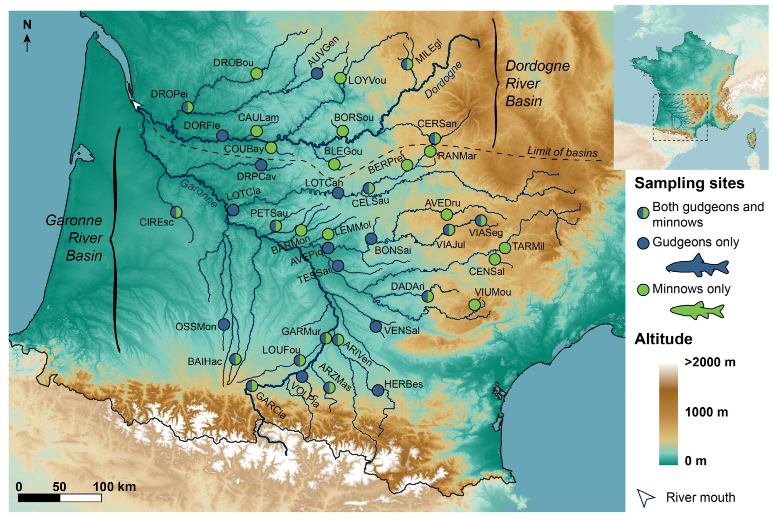
2.1. Study Area, Biological Models and Molecular Data

The study took place in two large river basins in southern France: the Garonne and the Dordogne watersheds. We focused on two abundant cyprinid species: the Garonne minnow Phoxinus dragarum [31] and the Languedoc gudgeon Gobio occitaniae [32]. These two cyprinid species are often found in sympatry, usually in fresh shallow waters. They are of similar maximal body length (200 and 140 mm, respectively) and they are both insectivorous, P. dragarum preferentially feeding in the water column and G. occitaniae at the bottom. Forty-two sites were sampled in 2011 and in 2014 with up to 30 adults from each species caught by electric fishing, resulting in a set of 35 and 37 sampled populations in minnows and gudgeons, respectively. On the field, a small piece of pelvic fin was collected from each individual and was preserved in 70% ethanol, before the fish were released in situ. Genomic DNA was extracted using a salt-extraction protocol [34] and used to obtain, for each species, individual-based STR genotypes from material collected in 2011, as well as population-based SNP allelic frequencies following a paired-end pool-seq procedure from material collected in 2014. The protocol used to produce STRs is detailed in [35], resulting in 17 and 13 loci in minnows and gudgeons, respectively, with no missing data. The protocol used to generate SNP allelic frequencies was very similar to the one detailed in [35], except that the reads were aligned to newly developed reference genomes rather than to draft genomes. The development of new reference genomes for P. dragarum and G. occitaniae is described in Appendix A and the protocol for the production of SNP allelic frequencies (i.e., the frequency in each population of the reference allele at each SNP) is detailed in Appendix B. SNP data were in the form of a data frame of allelic frequencies, with populations in rows and SNPs in columns. SNP data were iteratively cleaned as follows: we first discarded populations (i.e., rows) with more than 90% of SNPs with missing allelic frequency and then discarded any SNPs (i.e., columns) with missing allelic frequencies, resulting in 20,566 and 3039 SNPs (no missing data) in minnows and gudgeons, respectively. Since our study focused on comparing markers rather than comparing species, we randomly sampled 3000 SNPs (i.e., 3000 columns) in each species using the sample R-function. This subset had no influence on results (not shown). Finally, for each species, we retained populations for which we had both STRs and SNPs, resulting in a subset of 29 and 27 populations in minnows and gudgeons, respectively (Figure 1; Table 1), for a total of 41 unique populations (11 in the Dordogne and 30 in the Garonne watersheds, 15 with both minnows and gudgeons). Both STR individual genotypes and SNP allelic frequencies were converted into R-objects of class genpop (Table A1—row a) and were treated similarly in subsequent analyses. Genpop class objects contain allele counts for each locus in each population; SNP allele counts were obtained by multiplying allelic frequencies by twice the number of pooled individuals (Table 1).

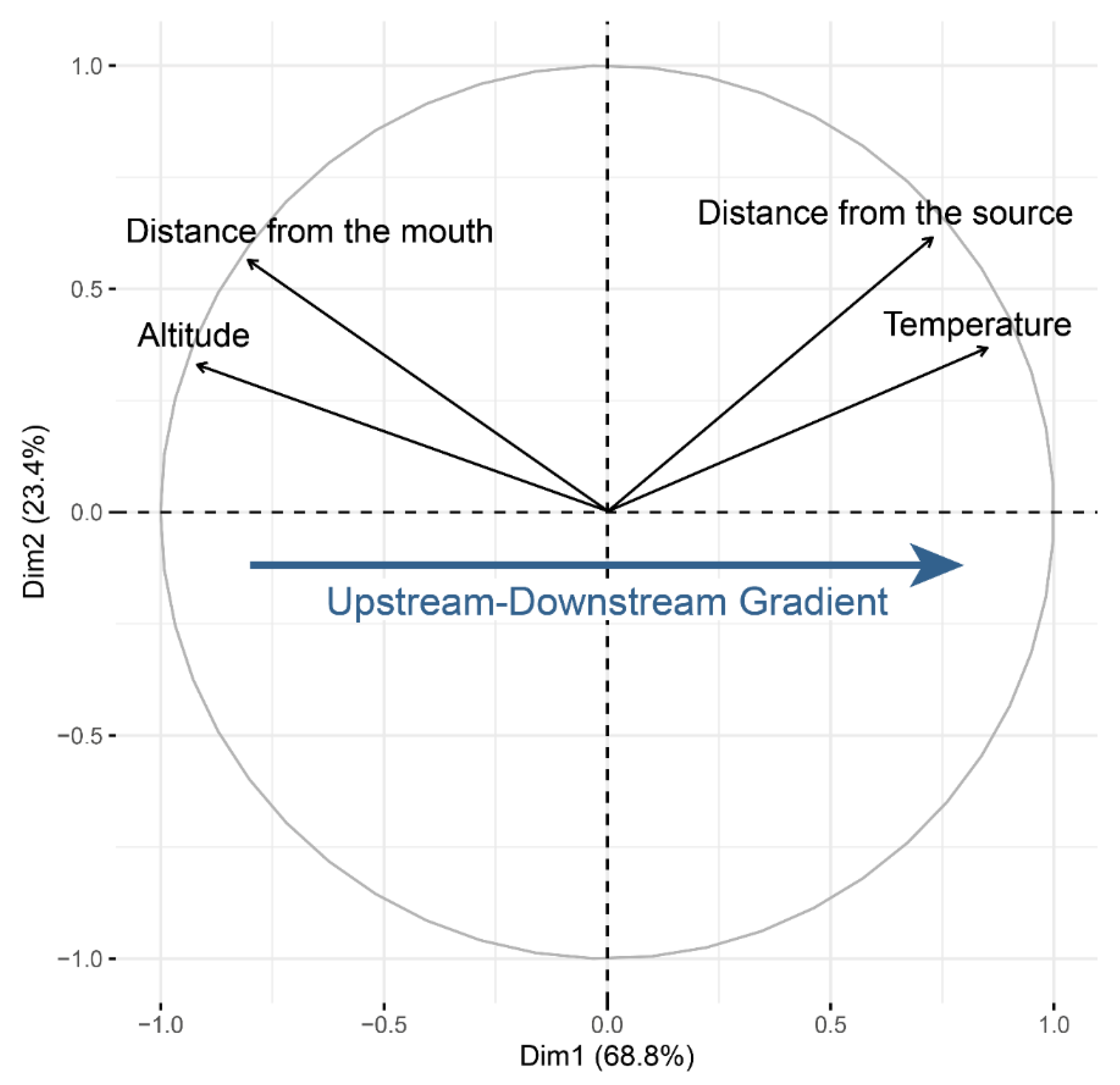
2.2. Environmental Data

We used public databases to characterize each population by its distance from the Garonne-Dordogne confluence (distance from the river mouth (DFM), in m), its distance from the source of the tributary it belonged to (DFS, in m), its altitude (in m) and its mean annual water temperature (in °C). Altitude and DFS were log-transformed to meet linearity assumptions. The four variables were synthetized into a unique environmental predictor using a principal component analysis (PCA; Table A1—row b). Missing temperatures (in BERPre and BONSai) were imputed beforehand using a regularized iterative PCA algorithm (Table A1—row c). Only the first principal component (PC) was retained, accounting for 68.8% of variance in environmental data and standing for an upstream–downstream gradient (UDG; Figure A1). For each species, we also computed the pairwise matrix of inter-population river distances (Table A1—row d).

2.3. Genetic Diversity and Spatial Patterns in Genetic Diversity

For each species and each marker, we first computed the expected heterozygosity He within each population (Table A1—row a). He is a fundamental measure of genetic diversity which derives directly from allelic frequencies [36] and which could therefore be calculated in a similar way for the two markers. He values were compared between markers using Pearson’s correlation coefficients (ρ; Table A1—row e).
To assess the precision of He, we performed the same calculations using a bootstrap procedure with 1000 iterations, randomly sampling loci with replacement at each iteration. The resulting bootstrapped distributions were sampled at quantiles 0.025 and 0.975 to obtain 95% confidence intervals CI95%. We also used these bootstrapped distributions to compute the coefficients of variation (CV) of He values, as the square root of the variance to mean ratio. To compare the precision of estimates between markers and species, we finally computed the mean ratio of precision in He estimates RHe (±SD) as follows:
R H e = m e a n ( C V S T R s / C V S N P s )
To determine whether we could similarly detect a significant downstream increase in genetic diversity (DIGD) in both species using both types of markers, we considered a single mixed model (Table A1—row f) with populations as a random term and the following fixed equation:
H e = S × M × U D G + U D G 2
With He as the measured expected heterozygosity, UDG as the score of populations along the upstream–downstream gradient, M as the type of marker (STRs or SNPs) and S as the species (gudgeons or minnows). The term UDG² was considered to capture putative quadratic trends in DIGD [37]. We used nested Type III ANOVA to assess the significance of interaction terms and discarded non-significant interactions while making sure that it did not degrade the model fit quality by investigating changes in Akaike criterion (AIC; Table A1—row e) and the normality of model residuals (Table A1—row g). For each fixed parameter of the final model, we computed CI95% using 1000 bootstrap iterations. Predicted He values were finally plotted against UDG for each type of marker and each species (Table A1—row h).

2.4. Genetic Differentiation and Isolation-by-Distance

For each species and each marker, we computed the pairwise matrix D of inter-population Nei’s genetic distances d [38] (Table A1—row a). Matrices D were then compared between markers using Mantel tests with 1000 permutations (Table A1—row i).
To assess the precision of pairwise measures d, we further computed 100 pairwise matrices D’ using a bootstrap procedure, randomly sampling loci with replacement at each iteration. The resulting bootstrapped distributions of d were sampled at quantiles 0.025 and 0.975 to obtain 95% confidence intervals CI95%. We also used these bootstrapped distributions to compute the coefficients of variation (CV) of d values, as the square root of the variance to mean ratio. To compare the precision of estimates between markers and species, we finally computed the mean ratio of precision in d estimates Rd (±SD) as follows:
R d = m e a n ( C V S T R s / C V S N P s )
To determine whether we could detect similar patterns of isolation-by-distance (IBD) from each type of marker in each species, we computed Mantel correlograms [39] (Table A1—row j), with each pairwise matrix of genetic distances D or D’ as the response variable, the corresponding pairwise matrix of inter-population river distances as a predictor and 1000 permutations. River distance classes were defined every 100 km. To assess the precision of IBD inferences, we sampled the distributions of Mantel correlations obtained from matrices D’ at quantiles 0.025 and 0.975 to obtain a CI95% about observed correlation values at each river distance class. Correlograms were then visually compared across markers in each species.

2.5. Genetic Structures

To compare spatial patterns of genetic variability as inferred from each marker in each species, we used two different approaches: hierarchical clustering and spatial principal component analyses (sPCA [40]). The goal of hierarchical clustering is to build a tree diagram where populations that are the most genetically similar are placed on branches that are close together. Pairwise matrices D were hierarchically clustered using the Ward’s clustering algorithm to minimize the total within-cluster variance [41] (Table A1—row e). For each species, trees were compared between marker types using the Baker’s Gamma correlation coefficient (γ; Table A1—row k) and visualized in the form of a tanglegram (one tree facing the other, with their labels connected by lines; Table A1—row k). The significance of γ was assessed using 1000 random permutations of population labels (Table A1—row k). To identify the optimal number k of clusters in each tree, we used the average silhouette method [42]: trees were cut into 2 to 20 clusters (Table A1—row l) and the value of k was identified as the one maximizing silhouette width (Table A1—row m).
We then used sPCAs (Table A1—row a). The goal of sPCA is to visualize spatial patterns of genetic variability by seeking principal components that optimize the variance of population allelic frequencies while taking the spatial autocorrelation of data into account. For each species, we used a network connecting each population to its n closest neighbors given pairwise river distances, with n chosen so as to minimize the number of neighbors while including all populations in the network (Table A1—row n). We used n = 3 in minnows and n = 4 in gudgeons, and only retained the two first PC from each sPCA, based on scree plot investigations. For each species and each retained PC, sPCA scores of populations were interpolated over the study area for visualization (Table A1—row o) and compared between markers using Pearson’s correlation coefficients (ρ).

3. Results

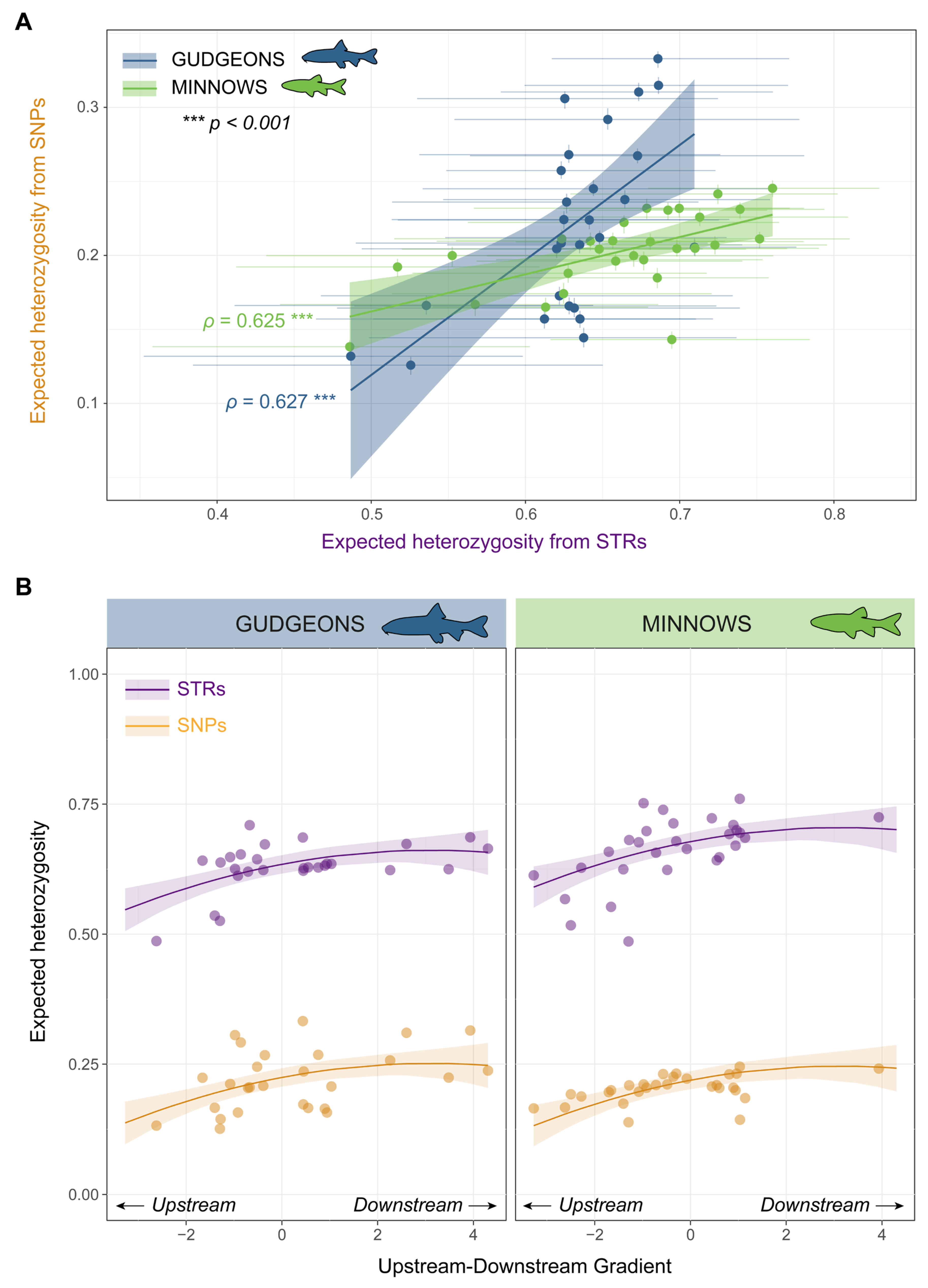
3.1. Genetic Diversity and Spatial Patterns in Genetic Diversity

Whatever the species, the precision of He estimates was about one order of magnitude (i.e., ~10-fold) higher with SNPs than with STRs (precision ratios RHe of 10.58 ± 1.51 and 8.01 ± 1.77, in gudgeons and minnows, respectively; error bars in Figure 2A). SNPs also yielded much lower He estimates than STRs (Table 2; marginal ‘SNP’ effect = −0.410). Nevertheless, He estimates were significantly correlated across markers (ρ > 0.62, p < 0.001; Figure 2A). Furthermore, similar DIGD patterns were identified whatever the species or the marker (Table 2 and Figure 2B); He increased downstreamward (marginal ‘UDG’ effect = 0.017), although this increase was less pronounced in the lower reaches (marginal ‘UDG²’ effect = −0.003).

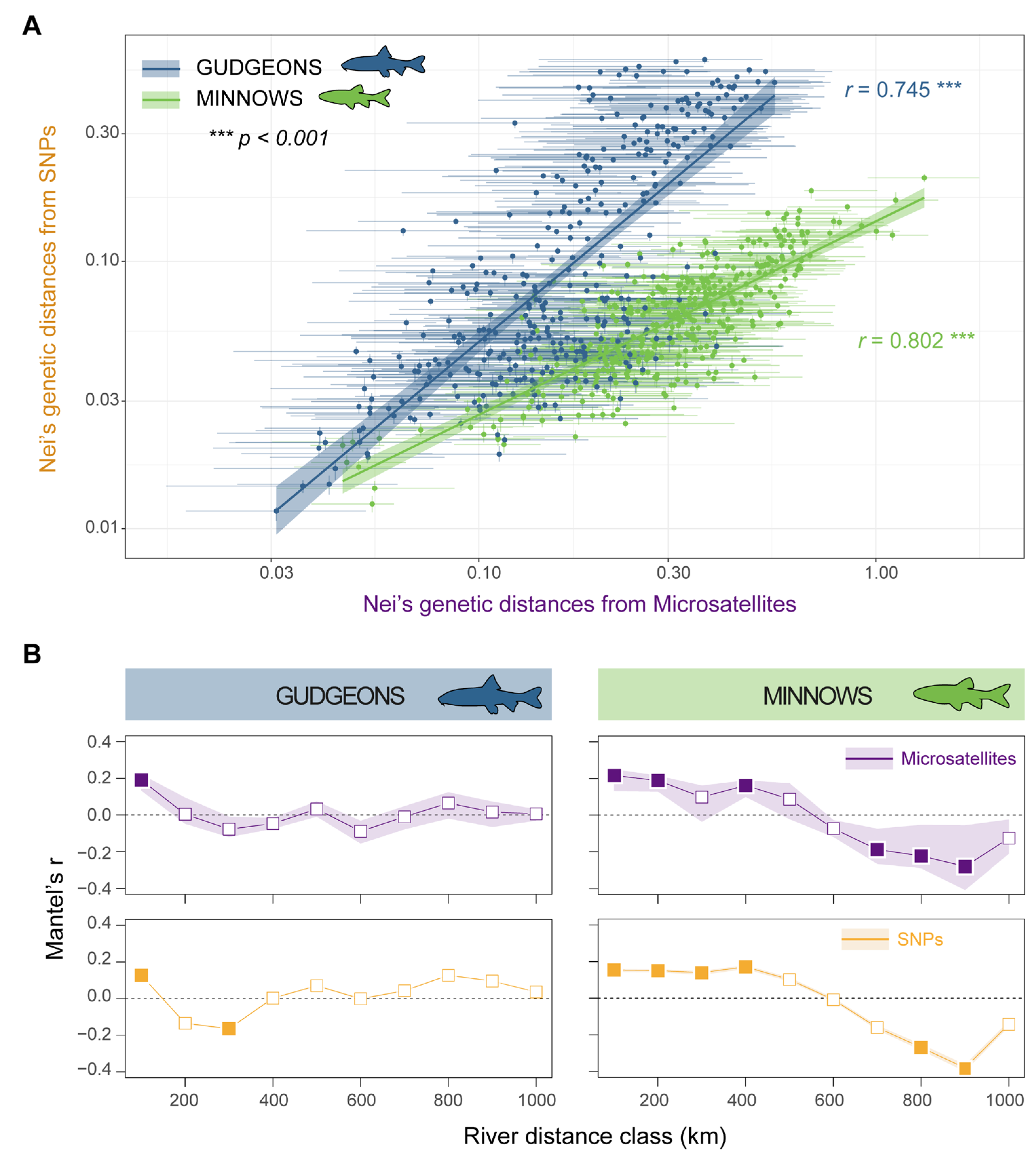
3.2. Genetic Differentiation and Isolation-by-Distance

As for He, the precision of estimates of pairwise measures of genetic distances d was about one order of magnitude higher with SNPs than with STRs, with a higher precision ratio obtained in gudgeons (Rd = 14.65 ± 4.10) than in minnows (Rd = 8.10 ± 1.76; error bars in Figure 3A). SNPs also yielded lower d estimates ( ln d S N P s = −2.62 ± 0.77) than STRs ( ln d S T R s = −1.48 ± 0.63; Figure 3A). Nevertheless, d estimates were significantly correlated across markers (r > 0.74, p < 0.001; Figure 3A). Furthermore, although the precision of SNP autocorrelograms was much higher than that of STRs (as indicated by the width of envelopes in Figure 3B), similar IBD patterns were identified in each species, whatever the marker: in gudgeons, populations showed significant genetic relatedness over the first 50–100 km (first river distance class), and no or negative autocorrelation at further distances; in minnows, populations showed significant genetic relatedness over the first 500–600 km (five first river distance classes), and no or negative autocorrelation at further distances (Figure 3B). The main discrepancy among markers was in minnows, with a non-significant Mantel’s r at the third distance class when using STRs.

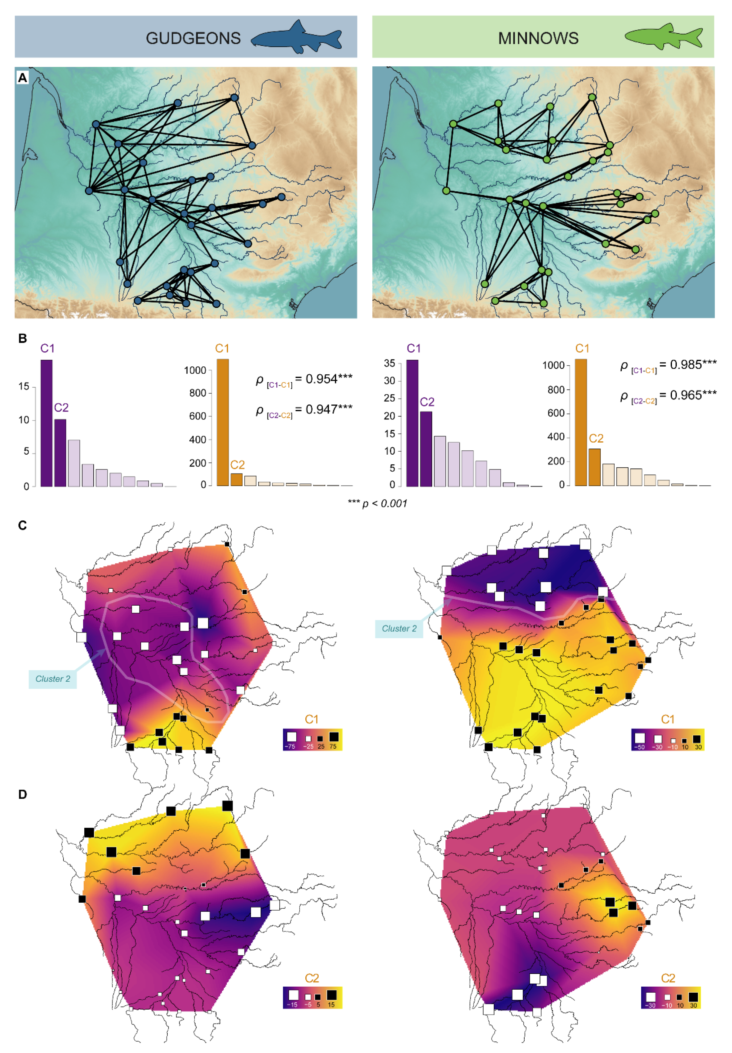
3.3. Genetic Structures

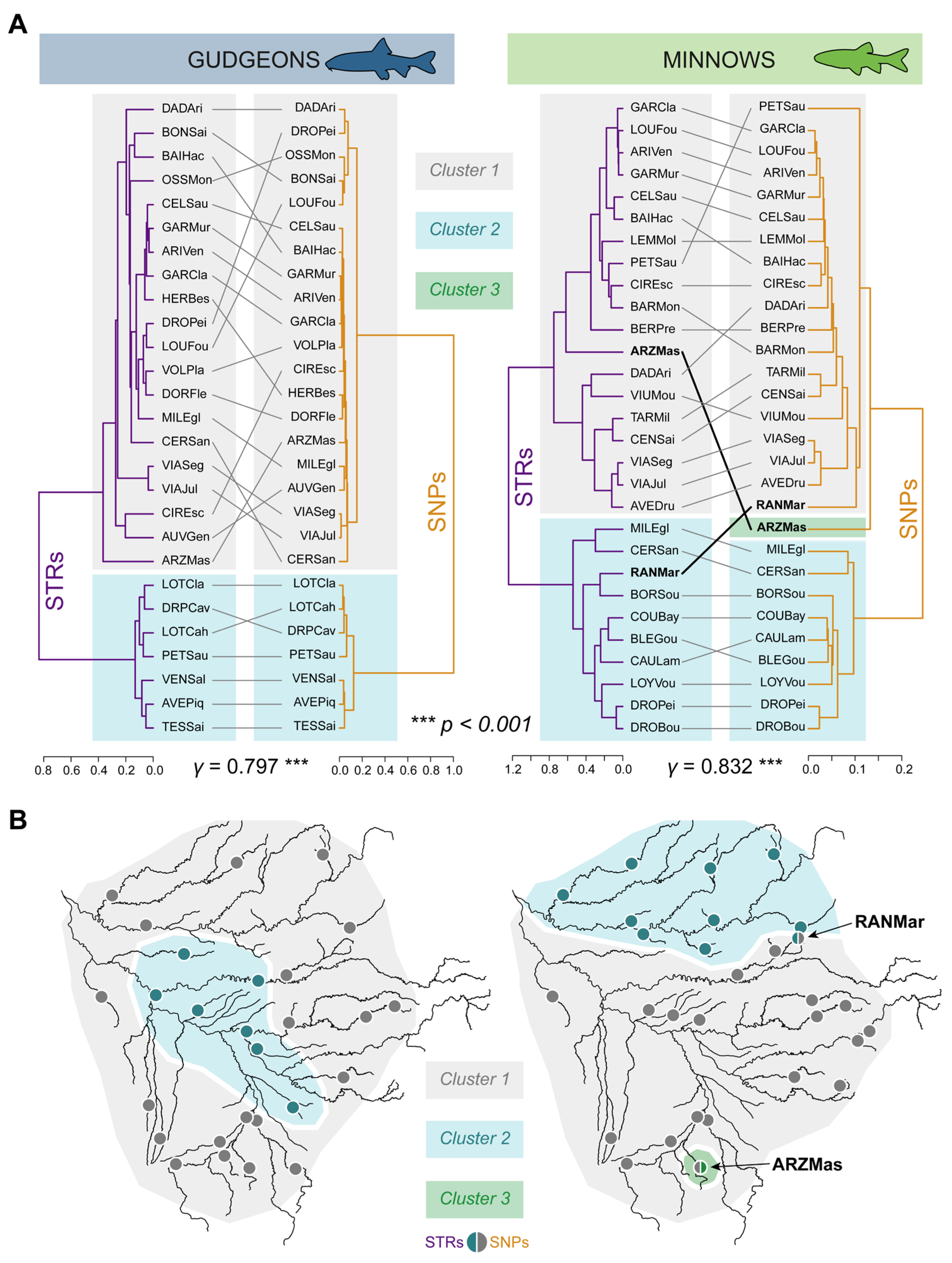
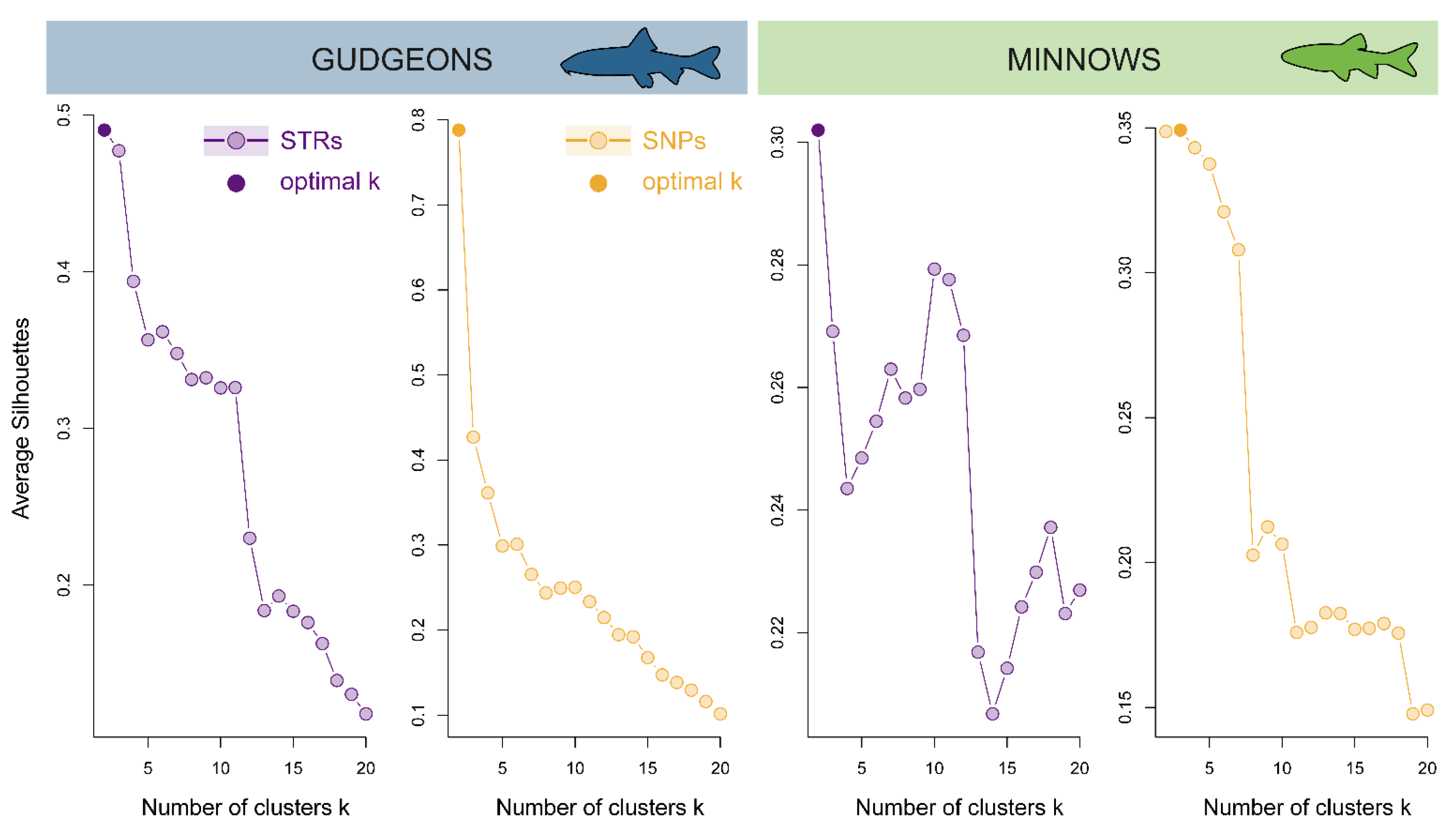
3.3.1. Hierarchical Clustering

In gudgeons, Wards’ hierarchical clustering trees computed from STRs and SNPs were highly correlated (γ = 0.797, p < 0.001), despite discrepancies in the positions of populations (Figure 4A). In both trees, the optimal number of clusters was k = 2 (Figure A2), with identical cluster compositions, and Cluster 2 comprised seven populations from the center of the Garonne River basin (Figure 4B). In minnows, Wards’ hierarchical clustering trees computed from STRs and SNPs were also highly correlated (γ = 0.832, p < 0.001), despite discrepancies in the positions of populations and a different optimal clustering. The optimal number of clusters was k = 2 in STRs and k = 3 in SNPs, although a value of k = 2 in SNPs was also highly supported by the data (Figure A2). Cluster 3 in SNPs comprised a single population, ARZMas, that was assigned to Cluster 1 when k = 2 (Figure 4A). Aside from this outlier population, the compositions of Clusters 1 and 2 were highly congruent, with Cluster 1 corresponding to the Garonne River basin and Cluster 2 to the Dordogne River basin. The only exception was the RANMar population, assigned to Cluster 2 with STRs but to Cluster 1 with SNPs (Figure 4A).

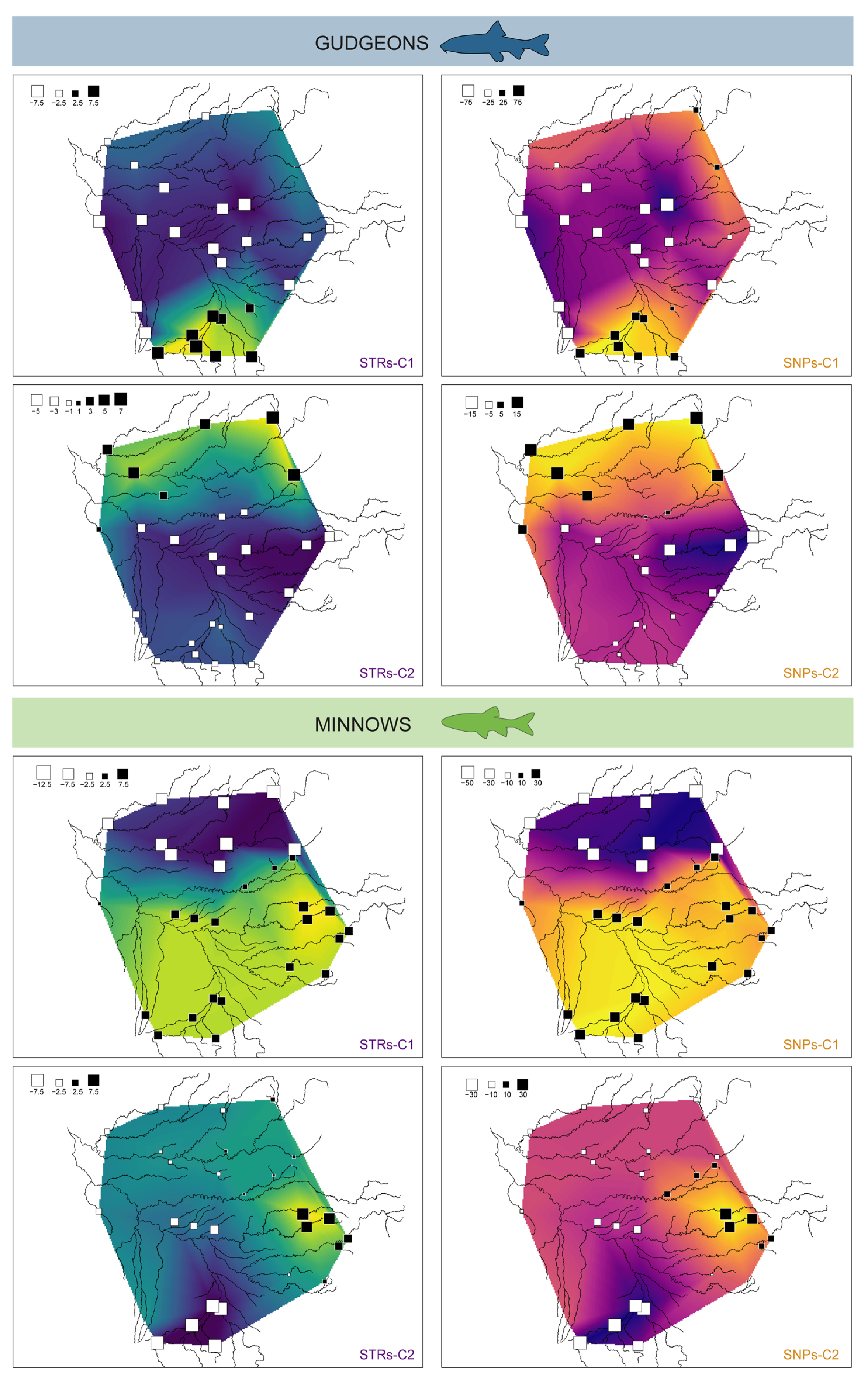
3.3.2. Spatial Principal Component Analyses

In both species, the two first sPCA components (PCs) from STRs and SNPs yielded highly correlated population scores (ρ > 0.94, p < 0.001; Figure 5B) and very similar spatial structures (Figure 5C,D and Figure A3). In gudgeons, the first PC (C1) segregated populations located in the southern upstream reaches of the Garonne River basin (populations with positive scores) from the rest of the basin, whereas populations from the Dordogne River basin showed little contribution to the PC (Figure 5C). This pattern partly coincided with the delineation of Cluster 2 inferred from Wards’ trees. The second PC (C2) distinguished the Dordogne River basin (positive scores) from the Garonne River basin, and specifically from populations located in the eastern upstream reaches of the Garonne River basin (Figure 5D). In minnows, the first PC (C1) differentiated the Dordogne River basin from the Garonne River basin (Figure 5C), in accordance with the clusters inferred from Wards’ trees. The second PC (C2) mostly segregated populations located in the eastern upstream reaches (positive scores) from populations located in the southern upstream reaches (negative scores) of the Garonne River basin.

4. Discussion

In our study, the main difference between SNPs and STRs was the precision of estimates of genetic diversity and genetic differentiation. In line with our expectations, estimates were one order of magnitude more precise with SNPs than with STRs, because of the much higher number of loci in SNPs than in STRs. The mean value of estimates of genetic diversity and genetic differentiation was also much lower in SNPs than in STRs, an expected outcome given differences in levels of polymorphism in each type of marker. These differences, however, had no influence on inferences regarding spatial patterns of genetic diversity, of isolation-by-distance and of genetic structuration, which were all highly congruent between markers. Our findings thus add to a growing body of scientific literature demonstrating that high-throughput markers such as SNPs might not be unconditionally superior to traditional approaches such as STRs in the context of genetic conservation [9,10].
Estimates of genetic diversity from each type of marker were significantly correlated and allowed the detection of similar patterns of downstream increase in genetic diversity (DIGD) in both species. DIGD is a classical pattern in river systems, stemming from the impoverishment of genetic pools in upstream areas through downstreamward asymmetrical gene flow and/or upstreamward recolonization from glacial refugees, and/or from the reduced influence of genetic drift in downstream areas where effective population sizes are usually larger [28,33]. The observed quadratic relationship between genetic diversity and distance from the source is also an expected pattern in river networks, which can be explained by their dendritic branching pattern [33,37]. Teasing apart the influence of DIGD from that of anthropogenic stressors (e.g., habitat fragmentation, hybridization with domestic strains, etc.) is crucial to properly planning conservation actions [37], and our results indicate that both types of markers were up to the task.
Pairwise estimates of genetic differentiation from each type of marker were also significantly correlated and allowed the detection of similar patterns of isolation-by-distance (IBD) in each species. Interestingly, the inferred IBD pattern was much more pronounced in gudgeons than in minnows, with genetic drift being much more influential than gene flow at distances higher than ~100 km in the former and at distances no less than ~400 km in the latter [43]. This difference in the spatial extent of migration-drift equilibrium may stem from several non-exclusive factors that would deserve further analyses: higher dispersal abilities and/or larger effective population sizes in minnows, species-specific responses to historical contingencies and/or anthropogenic stressors [43,44]. Nonetheless, regional conservation plans should probably take these distinct patterns into consideration when delineating conservation units [45].
The delineation of conservation units could, of course, also be informed through genetic structure analyses [46]. Here, we found that both types of markers revealed very similar genetic structures. Considering outputs from both sPCA and hierarchical clustering, at least three genetic clusters could be identified in each species: in gudgeons, the center of the Garonne River basin, the southern headwaters of the Garonne River basin (Pyrenees mountains), and the Dordogne River basin; in minnows, the Dordogne River basin, the eastern headwaters of the Garonne River basin (mountains of the “Massif Central”) and the southern headwaters of the Garonne River basin (Pyrenees mountains). At least two clusters corresponding to regional biogeographical features were thus common to both species: the Dordogne River basin and the Pyrenees mountains. These findings indicate that (i) the Garonne and the Dordogne river basins comprise rather independent genetic entities and that (ii) in the Garonne River basin, Pyrenean headwaters could be considered as a multi-species conservation unit, although the operational benefits of their preservation should of course be further evaluated [45]. The identification of Pyrenean headwaters as a putative conservation unit is in line with the reported disproportionate contribution of headwaters to biodiversity at the scale of river networks [47].
Interestingly, although STRs and SNPs provided very similar outcomes, we identified two discrepancies between markers in minnows’ hierarchical clustering. First, the ARZMas population was assigned to a cluster that was only detected using SNPs. This finding may suggest a higher resolution of SNPs in detecting subtle genetic structures [30]. However, given that SNPs were collected 3 years after STRs, we cannot exclude the probability that individuals from an unknown origin (captive-bred minnows, or minnows originating from another basin) were stocked in the meantime, for instance for recreational fishing, thus altering the genetic signature of the ARZMas population [37] between 2011 and 2014. Second, the RANMar population, located in the Garonne River basin, was surprisingly assigned to the “Dordogne” cluster using STRs, but not using SNPs. This finding could locally suggest a lack of resolution of STRs compared to SNPs, the modest number of STR loci not allowing the detection of specific genetic signatures in certain parts of the genome. However, as in the case of the ARZMas population, we cannot exclude the probability that individuals from the Dordogne River basin were stocked in the RANMar population (for instance, from the geographically very close CERSan population) before 2011, possibly just before the first sampling session. The fact that this “Dordogne” signature of the RANMar population was not detected with SNPs in 2014 could have resulted from the natural extirpation of allopatric strains within three years [48,49,50]. These two discrepancies could therefore be explained by unrecorded stocking events and are not sufficient to discredit STRs compared to SNPs without further investigation.
In this study, we assessed the genetic variability of two parapatric freshwater fish species on a relatively large spatial scale, with some populations located more than 900 km apart along the two considered river networks. We demonstrated that, at this scale, both STRs and SNPs yielded very similar results when considering population genetic analyses classically used in conservation genetics. At a finer spatial scale, of course, SNPs could have allowed the detection of subtle genetic structures that STRs might have missed [30], although our experience suggests that STRs remain relevant markers at inter-population distances of only a few hundred meters, as exemplified in other studies carried out within the Garonne River basin itself, particularly in the Célé (e.g., CELSau in Figure 1) and the Viaur rivers (VIAJul and VIASeg in Figure 1) [28,37]. SNPs can provide unprecedented opportunities, notably for the identification of adaptive patterns [13,18,22], but we join the growing number of researchers who defend the continued applicability of STRs in population genetic research, and in conservation genetics in particular [9,10,51]. This assertion is all the more important because, besides the fact that SNPs remain costly when a panel of STRs is already available (although pool-seq procedures and SNP panels can be highly cost-effective [17,52,53]), the production of SNPs requires bioinformatic expertise and computing power that may remain out of reach for some [10]. Moreover, some important issues, such as ascertainment biases ensuing from SNP discovery protocols [54,55,56], are still often overlooked (including in this very study), notably because (user-friendly) methods to circumvent them remain to be developed [57]. On the contrary, STRs benefit from decades of feedback, and we believe that they have definitely earned their place in the toolbox of researchers and managers, particularly in the case of riverscape studies [28].

Author Contributions

Conceptualization, J.G.P. and S.B.; methodology, J.G.P.; validation, S.B.; formal analysis, J.G.P.; resources, C.V., J.G.P. and G.L.; data curation, J.G.P.; writing—original draft preparation, J.G.P.; writing—review and editing, S.B.; visualization, J.G.P.; supervision, S.B.; project administration, S.B.; funding acquisition, S.B. All authors have read and agreed to the published version of the manuscript.

Funding

This work was financially supported by the Office Français pour la Biodiversité (OFB) and by the “Laboratoires d’Excellences (LABEX)” TULIP (ANR-10-LABX-41)”. The funders had no role in the design of the study, in the analyses or interpretation of data, in the writing of the manuscript or in the decision to publish the results. The OFB carried out part of the sampling in 2011 as part of their standard missions, and thus provided some samples.

Institutional Review Board Statement

Ethical review and approval were waived for this study due to the use of already published data.

Data Availability Statement

Data used in this study are available on FigShare (https://0-doi-org.brum.beds.ac.uk/10.6084/m9.figshare.22309753.v1; accessed on 17 May 2023).

Acknowledgments

We warmly thank all the colleagues and students who helped with field sampling in 2011 and 2014. We are also grateful to Romain Derelle and Rik Verdonck for their advice with genome assemblies.

Conflicts of Interest

The authors declare no conflict of interest.

Appendix A. Genome Assembly

In each species (Phoxinus dragarum and Gobio occitaniae), a piece of muscle was collected from a single individual that was sampled as described in the main text and euthanized by benzocaine overdose. After DNA extraction as described in the main text, high-fidelity (HiFi) long reads were produced by the Gentyane company (Clermont-Ferrand, France) for G. occitaniae and the Novogene (UK) Company Limited (Cambridge, UK) for P. dragarum using Sequel 8M PacBio systems [58]. Circular consensus sequences (CCS) were generated using the ccs script (Table A1—row p) and the resulting bam files were converted to fastq files using bedtools (Table A1—row q). Genome assemblies were produced using hicanu (Table A1—row r), with an estimated genome-size of 1125 Mb for P. dragarum and 1555 Mb for G. occitaniae [59], a high sensitivity level, a corrected error rate of 0.055, a correction of all reads (corOutCoverage = 999) and a coverage cutoff of 5 (stopOnLowCoverage = 5). Assembly fastq files were manipulated using SeqKit (Table A1—row s) to discard repeat, bubble and circular sequences and were curated using purge_haplotigs (Table A1—row t). Finally, we used BUSCO for a quantitative assessment of final genome assemblies, with the actinopterygii_odb10 database in both species (Table A1—row u).
The following table provides the main characteristics of the final assemblies. Note that the G. occitaniae assembly showed a higher proportion of BUSCO duplicates than the P. dragarum assembly (20% against 4%), but that the proportion of missing or fragmented BUSCOs was higher in G. occitaniae than in P. dragarum (12.2% against 6.8%).
Phoxinus dragarumGobio occitaniae
Localization of specimens (Lat. Long.)42.958 N 1.085 E42.921 N 1.898 E
Accession numberJARPMJ000000000JARQWZ000000000
Assembly nameCNRS_Phodra_1.0CNRS_Gobocc_1.0
Assembly size (Mb)968.11721.8
% missing bases00
% GC39.1439.99
Number of contigs10,13710,985
Number of contigs > 100 kb31004833
N50 contig length (kb)128.19315.98
Shortest contig13,9208919
Longest contig1,089,8742,163,237
Complete BUSCOs3195 (87.8%)3394 (93.2%)
Complete and single-copy BUSCOs3050 (83.8%)2666 (73.2%)
Complete and duplicated BUSCOs145 (4%)728 (20.0%)
Fragmented BUSCOs117 (3.2%)86 (2.4%)
Missing BUSCOs328 (9%)160 (4.4%)
Total BUSCO groups searched3640 (100%)3640 (100%)

Appendix B. Production of SNP Allelic Frequencies

For each species and each station, DNA from all individuals was pooled at equimolar concentrations to reach a total amount of 5 mg of DNA, according to individual concentrations measured using a QuBit 2.0 fluorometer (2.0; Life Technologies, Carlsbad, CA, USA). Pooled DNA from each species and each station was homogenized and digested using SbfI restriction enzymes, followed by barcode ligation, sample pooling, DNA shearing, size selection of RAD tags (150 bp), adaptor ligation, RAD tag amplification and sequencing on two Hiseq lanes (GeT Platform, Toulouse, France). Resulting demultiplexed paired-end short reads were filtered using the process_radtags and the clone_filter functions from Stacks [60], in order to remove reads with uncalled bases or low-quality scores and discard PCR duplicates. Filtered reads were then aligned on the corresponding reference genome using the mem function from BWA [61]. Aligned SAM files were converted to BAM format with the view and sort functions from SamTools [62], and filtered for unpaired, unmapped or badly mapped reads (mapping quality score < 20) using the filter function from BamTools [63]. For each species, all indexed and filtered BAM files were then assembled in a single mpileup file using the mpileup function from SamTools. These mpileup files were synchronized in Popoolation2 [64] with the mpileup2sync.jar java script. Finally, SNP allelic frequencies were determined using the snp-frequency-diff.pl perl script in Popoolation2 with a minimum allele count of 4 and a coverage ranging from 30 to 400.
Table A1. Main resources (R-packages or conda/github-repository) and associated functions/scripts used in this study.
In-Text ReferenceResourcesFunctions/ScriptsReference
aR-adegenetas.genpop, Hs, dist.genpop, spca[65]
bR-factoMineRPCA[66]
cR-missMDAimputePCA[67]
dR-riverdistriverdistancemat[68]
eR-statscor.test, AIC, hclust[69]
fR-glmmTMBglmmTMB[70]
gR-DHARMasimulateResiduals [71]
hR-sjPlotplot_model[72]
iR-veganmantel[73]
jR-mpmcorrelogrammpmcorrelogram[74]
kR-dendextendcor_bakers_gamma, untangle, tantelgram, sample.dendrogram[75]
lR-factoextrahcut[76]
mR-clustersilhouette[77]
nR-evclustknn.dist[78]
oR-interpinterp[79]
pgithub-PacificBiosciencesccs[58]
qconda-bedtools [80]
rgithub-marlcanu[81]
sconda-SeqKitseq, grep[82]
tconda-purge_haplotigshist, cov, purge[83]
uconda-BUSCObusco[84]
Figure A1. Creation of the upstream-downstream gradient (UDG) variable.
Diversity 15 00681 g0a1
A representation of the two first principal components (PCs) was used to synthetize environmental data. Only the first PC was retained, accounting for 68.8% of variability in environmental data. It distinguished populations located at high altitude and far from the river mouth (upstream populations, also characterized by cooler water temperatures) from populations located in warmer water temperatures and far from the source of tributaries they belong to (downstream populations, also characterized by lower altitudes).
Figure A2. Determination of the optimal number k of clusters in each Wards’ hierarchical tree using the average silhouette method.
Diversity 15 00681 g0a2
For each species and each type of marker, the average tree silhouette width for a number of clusters k varying from 2 to 20 was calculated. In gudgeons and in the tree based on STRs in minnows, the optimal number of clusters was 2. In the tree based on SNPs in minnows, the optimal number of clusters was 3 (width = 0.3492), but a value of 2 was also highly supported (width = 0.3487).
Figure A3. sPCA outputs for each species, each marker (STRs or SNPs) and each retained component (C1 or C2). Large white (dark blue or purple background in STRs and SNPs, respectively) and black (yellow background) squares stand for highly negative and positive scores, respectively. Small squares stand for small sPCA scores.
Diversity 15 00681 g0a3

References

  1. Steffen, W.; Grinevald, J.; Crutzen, P.; McNeill, J. The Anthropocene: Conceptual and historical perspectives. Philos. Trans. R. Soc. Math. Phys. Eng. Sci. 2011, 369, 842–867. [Google Scholar] [CrossRef] [PubMed]
  2. Miraldo, A.; Li, S.; Borregaard, M.K.; Flórez-Rodríguez, A.; Gopalakrishnan, S.; Rizvanovic, M.; Wang, Z.; Rahbek, C.; Marske, K.A.; Nogués-Bravo, D. An Anthropocene map of genetic diversity. Science 2016, 353, 1532–1535. [Google Scholar] [CrossRef] [PubMed]
  3. Margules, C.R.; Pressey, R.L. Systematic conservation planning. Nature 2000, 405, 243–253. [Google Scholar] [CrossRef] [PubMed]
  4. Diniz-Filho, J.A.F.; Melo, D.B.; de Oliveira, G.; Collevatti, R.G.; Soares, T.N.; Nabout, J.C.; de Souza Lima, J.; Dobrovolski, R.; Chaves, L.J.; Naves, R.V.; et al. Planning for optimal conservation of geographical genetic variability within species. Conserv. Genet. 2012, 13, 1085–1093. [Google Scholar] [CrossRef]
  5. Paz-Vinas, I.; Loot, G.; Hermoso, V.; Veyssiere, C.; Poulet, N.; Grenouillet, G.; Blanchet, S. Systematic conservation planning for intraspecific genetic diversity. bioRxiv 2018. bioRxiv:105544. [Google Scholar] [CrossRef]
  6. Comte, L.; Olden, J.D. Fish dispersal in flowing waters: A synthesis of movement- and genetic-based studies. Fish Fish. 2018, 19, 1063–1077. [Google Scholar] [CrossRef]
  7. Pertoldi, C.; Bijlsma, R.; Loeschcke, V. Conservation genetics in a globally changing environment: Present problems, paradoxes and future challenges. Biodivers. Conserv. 2007, 16, 4147–4163. [Google Scholar] [CrossRef]
  8. Sarre, S.D.; Georges, A. Genetics in conservation and wildlife management: A revolution since Caughley. Wildl. Res. 2009, 36, 70. [Google Scholar] [CrossRef]
  9. Schlötterer, C. The evolution of molecular markers—Just a matter of fashion? Nat. Rev. Genet. 2004, 5, 63–69. [Google Scholar] [CrossRef]
  10. Hauser, S.S.; Athrey, G.; Leberg, P.L. Waste not, want not: Microsatellites remain an economical and informative technology for conservation genetics. Ecol. Evol. 2021, 11, 15800–15814. [Google Scholar] [CrossRef]
  11. Putman, A.I.; Carbone, I. Challenges in analysis and interpretation of microsatellite data for population genetic studies. Ecol. Evol. 2014, 4, 4399–4428. [Google Scholar] [CrossRef]
  12. Morin, P.A.; Luikart, G.; Wayne, R.K.; the SNP Workshop Group. SNPs in ecology, evolution and conservation. Trends Ecol. Evol. 2004, 19, 208–216. [Google Scholar] [CrossRef]
  13. Zimmerman, S.J.; Aldridge, C.L.; Oyler-McCance, S.J. An empirical comparison of population genetic analyses using microsatellite and SNP data for a species of conservation concern. BMC Genom. 2020, 21, 382. [Google Scholar] [CrossRef] [PubMed]
  14. Brumfield, R.T.; Beerli, P.; Nickerson, D.A.; Edwards, S.V. The utility of single nucleotide polymorphisms in inferences of population history. Trends Ecol. Evol. 2003, 18, 249–256. [Google Scholar] [CrossRef]
  15. Seddon, J.M.; Parker, H.G.; Ostrander, E.A.; Ellegren, H. SNPs in ecological and conservation studies: A test in the Scandinavian wolf population. Mol. Ecol. 2005, 14, 503–511. [Google Scholar] [CrossRef]
  16. Puckett, E.E. Variability in total project and per sample genotyping costs under varying study designs including with microsatellites or SNPs to answer conservation genetic questions. Conserv. Genet. Resour. 2017, 9, 289–304. [Google Scholar] [CrossRef]
  17. Schlötterer, C.; Tobler, R.; Kofler, R.; Nolte, V. Sequencing pools of individuals—Mining genome-wide polymorphism data without big funding. Nat. Rev. Genet. 2014, 15, 749–763. [Google Scholar] [CrossRef] [PubMed]
  18. McMahon, B.J.; Teeling, E.C.; Höglund, J. How and why should we implement genomics into conservation? Evol. Appl. 2014, 7, 999–1007. [Google Scholar] [CrossRef]
  19. Muñoz, I.; Henriques, D.; Jara, L.; Johnston, J.S.; Chávez-Galarza, J.; De La Rúa, P.; Pinto, M.A. SNPs selected by information content outperform randomly selected microsatellite loci for delineating genetic identification and introgression in the endangered dark European honeybee (Apis mellifera mellifera). Mol. Ecol. Resour. 2017, 17, 783–795. [Google Scholar] [CrossRef]
  20. Dziech, A. Identification of Wolf-Dog Hybrids in Europe—An Overview of Genetic Studies. Front. Ecol. Evol. 2021, 9, 760160. [Google Scholar] [CrossRef]
  21. Flanagan, S.P.; Jones, A.G. The future of parentage analysis: From microsatellites to SNPs and beyond. Mol. Ecol. 2019, 28, 544–567. [Google Scholar] [CrossRef]
  22. Allendorf, F.W.; Hohenlohe, P.A.; Luikart, G. Genomics and the future of conservation genetics. Nat. Rev. Genet. 2010, 11, 697–709. [Google Scholar] [CrossRef]
  23. Shafer, A.B.A.; Wolf, J.B.W.; Alves, P.C.; Bergström, L.; Bruford, M.W.; Brännström, I.; Colling, G.; Dalén, L.; De Meester, L.; Ekblom, R.; et al. Genomics and the challenging translation into conservation practice. Trends Ecol. Evol. 2015, 30, 78–87. [Google Scholar] [CrossRef]
  24. Theissinger, K.; Fernandes, C.; Formenti, G.; Bista, I.; Berg, P.R.; Bleidorn, C.; Bombarely, A.; Crottini, A.; Gallo, G.R.; Godoy, J.A.; et al. How genomics can help biodiversity conservation. Trends Genet. 2023, S0168952523000203. [Google Scholar] [CrossRef] [PubMed]
  25. Meybeck, M. Global analysis of river systems: From Earth system controls to Anthropocene syndromes. Philos. Trans. R. Soc. Lond. B Biol. Sci. 2003, 358, 1935–1955. [Google Scholar] [CrossRef] [PubMed]
  26. Reid, A.J.; Carlson, A.K.; Creed, I.F.; Eliason, E.J.; Gell, P.A.; Johnson, P.T.J.; Kidd, K.A.; MacCormack, T.J.; Olden, J.D.; Ormerod, S.J.; et al. Emerging threats and persistent conservation challenges for freshwater biodiversity. Biol. Rev. 2018, 94, 849–873. [Google Scholar] [CrossRef] [PubMed]
  27. Davis, C.D.; Epps, C.W.; Flitcroft, R.L.; Banks, M.A. Refining and defining riverscape genetics: How rivers influence population genetic structure. Wiley Interdiscip. Rev. Water 2018, 5, e1269. [Google Scholar] [CrossRef]
  28. Blanchet, S.; Prunier, J.G.; Paz-Vinas, I.; Saint-Pé, K.; Rey, O.; Raffard, A.; Mathieu-Bégné, E.; Loot, G.; Fourtune, L.; Dubut, V. A river runs through it: The causes, consequences, and management of intraspecific diversity in river networks. Evol. Appl. 2020, 13, 1195–1213. [Google Scholar] [CrossRef]
  29. Morgan, T.D.; Graham, C.F.; McArthur, A.G.; Raphenya, A.R.; Boreham, D.R.; Manzon, R.G.; Wilson, J.Y.; Lance, S.L.; Howland, K.L.; Patrick, P.H.; et al. Genetic population structure of the round whitefish (Prosopium cylindraceum) in North America: Multiple markers reveal glacial refugia and regional subdivision. Can. J. Fish. Aquat. Sci. 2018, 75, 836–849. [Google Scholar] [CrossRef]
  30. Dufresnes, C.; Dutoit, L.; Brelsford, A.; Goldstein-Witsenburg, F.; Clément, L.; López-Baucells, A.; Palmeirim, J.; Pavlinić, I.; Scaravelli, D.; Ševčík, M.; et al. Inferring genetic structure when there is little: Population genetics versus genomics of the threatened bat Miniopterus schreibersii across Europe. Sci. Rep. 2023, 13, 1523. [Google Scholar] [CrossRef]
  31. Denys, G.P.J.; Dettai, A.; Persat, H.; Daszkiewicz, P.; Hautecœur, M.; Keith, P. Revision of Phoxinus in France with the description of two new species (Teleostei, Leuciscidae). Cybium 2020, 44, 205–237. [Google Scholar] [CrossRef]
  32. Kottelat, M.; Persat, H. The genus Gobio in France, with redescription of G. gobio and description of two new species (Teleostei: Cyprinidae). Cybium 2005, 29, 211–234. [Google Scholar]
  33. Paz-Vinas, I.; Blanchet, S. Dendritic connectivity shapes spatial patterns of genetic diversity: A simulation-based study. J. Evol. Biol. 2015, 28, 986–994. [Google Scholar] [CrossRef] [PubMed]
  34. Aljanabi, S.M.; Martinez, I. Universal and rapid salt-extraction of high quality genomic DNA for PCR-based techniques. Nucleic Acids Res. 1997, 25, 4692–4693. [Google Scholar] [CrossRef] [PubMed]
  35. Prunier, J.G.; Chevalier, M.; Raffard, A.; Loot, G.; Poulet, N.; Blanchet, S. Genetic erosion reduces biomass temporal stability in wild fish populations. bioRxiv 2023. [Google Scholar] [CrossRef]
  36. Nei, M. Analysis of gene diversity in subdivided populations. Proc. Natl. Acad. Sci. USA 1973, 70, 3321–3323. [Google Scholar] [CrossRef]
  37. Prunier, J.G.; Dubut, V.; Loot, G.; Tudesque, L.; Blanchet, S. The relative contribution of river network structure and anthropogenic stressors to spatial patterns of genetic diversity in two freshwater fishes: A multiple-stressors approach. Freshw. Biol. 2018, 63, 6–21. [Google Scholar] [CrossRef]
  38. Nei, M. Genetic Distance between Populations. Am. Nat. 1972, 106, 283–292. [Google Scholar] [CrossRef]
  39. Sokal, R.R.; Smouse, P.E.; Neel, J.V. The genetic structure of a tribal population, the Yanomama Indians. XV. Patterns inferred by autocorrelation analysis. Genetics 1986, 114, 259–287. [Google Scholar] [CrossRef]
  40. Jombart, T.; Devillard, S.; Dufour, A.B.; Pontier, D. Revealing cryptic spatial patterns in genetic variability by a new multivariate method. Heredity 2008, 101, 92–103. [Google Scholar] [CrossRef]
  41. Ward, J.H. Hierarchical Grouping to Optimize an Objective Function. J. Am. Stat. Assoc. 1963, 58, 236–244. [Google Scholar] [CrossRef]
  42. Rousseeuw, P.J. Silhouettes: A graphical aid to the interpretation and validation of cluster analysis. J. Comput. Appl. Math. 1987, 20, 53–65. [Google Scholar] [CrossRef]
  43. Hutchison, D.W.; Templeton, A.R. Correlation of Pairwise Genetic and Geographic Distance Measures: Inferring the Relative Influences of Gene Flow and Drift on the Distribution of Genetic Variability. Evolution 1999, 53, 1898. [Google Scholar] [CrossRef] [PubMed]
  44. van Strien, M.J.; Holderegger, R.; Van Heck, H.J. Isolation-by-distance in landscapes: Considerations for landscape genetics. Heredity 2015, 114, 27–37. [Google Scholar] [CrossRef] [PubMed]
  45. Paz-Vinas, I.; Loot, G.; Hermoso, V.; Veyssière, C.; Poulet, N.; Grenouillet, G.; Blanchet, S. Systematic conservation planning for intraspecific genetic diversity. Proc. R. Soc. B Biol. Sci. 2018, 285, 20172746. [Google Scholar] [CrossRef] [PubMed]
  46. Paetkau, D. Using Genetics to Identify Intraspecific Conservation Units: A Critique of Current Methods. Conserv. Biol. 1999, 13, 1507–1509. [Google Scholar] [CrossRef]
  47. Finn, D.S.; Bonada, N.; Múrria, C.; Hughes, J.M. Small but mighty: Headwaters are vital to stream network biodiversity at two levels of organization. J. North Am. Benthol. Soc. 2011, 30, 963–980. [Google Scholar] [CrossRef]
  48. Saint-Pé, K.; Blanchet, S.; Tissot, L.; Poulet, N.; Plasseraud, O.; Loot, G.; Veyssière, C.; Prunier, J.G. Genetic admixture between captive-bred and wild individuals affects patterns of dispersal in a brown trout (Salmo trutta) population. Conserv. Genet. 2018, 19, 1269–1279. [Google Scholar] [CrossRef]
  49. Diana, M.J.; Wahl, D.H. Growth and Survival of Four Sizes of Stocked Largemouth Bass. North Am. J. Fish. Manag. 2009, 29, 1653–1663. [Google Scholar] [CrossRef]
  50. Prunier, J.G.; Saint-Pé, K.; Tissot, L.; Poulet, N.; Marselli, G.; Veyssière, C.; Blanchet, S. Captive-bred ancestry affects spatial patterns of genetic diversity and differentiation in brown trout (Salmo trutta) populations. Aquat. Conserv. Mar. Freshw. Ecosyst. 2022, 32, 1529–1543. [Google Scholar] [CrossRef]
  51. Narum, S.R.; Banks, M.; Beacham, T.D.; Bellinger, M.R.; Campbell, M.R.; Dekoning, J.; Elz, A.; Guthrieiii, C.M.; Kozfkay, C.; Miller, K.M.; et al. Differentiating salmon populations at broad and fine geographical scales with microsatellites and single nucleotide polymorphisms. Mol. Ecol. 2008, 17, 3464–3477. [Google Scholar] [CrossRef]
  52. Roques, S.; Chancerel, E.; Boury, C.; Pierre, M.; Acolas, M. From microsatellites to single nucleotide polymorphisms for the genetic monitoring of a critically endangered sturgeon. Ecol. Evol. 2019, 9, 7017–7029. [Google Scholar] [CrossRef] [PubMed]
  53. Saint-Pé, K.; Leitwein, M.; Tissot, L.; Poulet, N.; Guinand, B.; Berrebi, P.; Marselli, G.; Lascaux, J.-M.; Gagnaire, P.-A.; Blanchet, S. Development of a large SNPs resource and a low-density SNP array for brown trout (Salmo trutta) population genetics. BMC Genom. 2019, 20, 582. [Google Scholar] [CrossRef] [PubMed]
  54. O’Leary, S.J.; Puritz, J.B.; Willis, S.C.; Hollenbeck, C.M.; Portnoy, D.S. These aren’t the loci you’e looking for: Principles of effective SNP filtering for molecular ecologists. Mol. Ecol. 2018, 27, 3193–3206. [Google Scholar] [CrossRef] [PubMed]
  55. Nielsen, R.; Signorovitch, J. Correcting for ascertainment biases when analyzing SNP data: Applications to the estimation of linkage disequilibrium. Theor. Popul. Biol. 2003, 63, 245–255. [Google Scholar] [CrossRef] [PubMed]
  56. Schmidt, T.L.; Jasper, M.; Weeks, A.R.; Hoffmann, A.A. Unbiased population heterozygosity estimates from genome-wide sequence data. Methods Ecol. Evol. 2021, 12, 1888–1898. [Google Scholar] [CrossRef]
  57. Dokan, K.; Kawamura, S.; Teshima, K.M. Effects of single nucleotide polymorphism ascertainment on population structure inferences. G3 GenesGenomesGenetics 2021, 11, jkab128. [Google Scholar] [CrossRef]
  58. Wenger, A.M.; Peluso, P.; Rowell, W.J.; Chang, P.-C.; Hall, R.J.; Concepcion, G.T.; Ebler, J.; Fungtammasan, A.; Kolesnikov, A.; Olson, N.D.; et al. Accurate circular consensus long-read sequencing improves variant detection and assembly of a human genome. Nat. Biotechnol. 2019, 37, 1155–1162. [Google Scholar] [CrossRef]
  59. Gregory, T.R. Animal Genome Size Database. 2002. Available online: http://www.genomesize.com (accessed on 1 October 2021).
  60. Catchen, J.; Hohenlohe, P.A.; Bassham, S.; Amores, A.; Cresko, W.A. Stacks: An analysis tool set for population genomics. Mol. Ecol. 2013, 22, 3124–3140. [Google Scholar] [CrossRef]
  61. Li, H.; Durbin, R. Fast and accurate short read alignment with Burrows-Wheeler transform. Bioinformatics 2009, 25, 1754–1760. [Google Scholar] [CrossRef]
  62. Li, H.; Handsaker, B.; Wysoker, A.; Fennell, T.; Ruan, J.; Homer, N.; Marth, G.; Abecasis, G.; Durbin, R. 1000 Genome Project Data Processing Subgroup The Sequence Alignment/Map format and SAMtools. Bioinformatics 2009, 25, 2078–2079. [Google Scholar] [CrossRef]
  63. Barnett, D.W.; Garrison, E.K.; Quinlan, A.R.; Stromberg, M.P.; Marth, G.T. BamTools: A C++ API and toolkit for analyzing and managing BAM files. Bioinformatics 2011, 27, 1691–1692. [Google Scholar] [CrossRef]
  64. Kofler, R.; Pandey, R.V.; Schlötterer, C. PoPoolation2: Identifying differentiation between populations using sequencing of pooled DNA samples (Pool-Seq). Bioinformatics 2011, 27, 3435–3436. [Google Scholar] [CrossRef]
  65. Jombart, T. adegenet: A R package for the multivariate analysis of genetic markers. Bioinformatics 2008, 24, 1403–1405. [Google Scholar] [CrossRef]
  66. Lê, S.; Josse, J.; Husson, F. FactoMineR: An R Package for Multivariate Analysis. J. Stat. Softw. 2008, 25, 1–18. [Google Scholar] [CrossRef]
  67. Josse, J.; Husson, F. missMDA: A Package for Handling Missing Values in Multivariate Data Analysis. J. Stat. Softw. 2016, 70, 1–31. [Google Scholar] [CrossRef]
  68. Tyers, M. Riverdist: River Network Distance Computation and Applications; R Package Version 0.14. 0; R Foundation for Statistical Computing: Vienna, Austria, 2017. [Google Scholar]
  69. R Core Team. R: A Language and Environment for Statistical Computing; R Foundation for Statistical Computing, Vienna, Austria. 2022. Available online: https://www.R-project.org/ (accessed on 17 May 2023).
  70. Brooks, M.E.; Kristensen, K.; Benthem, K.J.; van Magnusson, A.; Berg, C.W.; Nielsen, A.; Skaug, H.J.; Mächler, M.; Bolker, B.M. glmmTMB Balances Speed and Flexibility Among Packages for Zero-inflated Generalized Linear Mixed Modeling. R J. 2017, 9, 378. [Google Scholar] [CrossRef]
  71. Hartig, F. DHARMa: Residual Diagnostics for Hierarchical (Multi-Level/Mixed) Regression Models_; R Package Version 0.4.6; R Foundation for Statistical Computing: Vienna, Austria, 2022. [Google Scholar]
  72. Lüdecke, D. sjPlot: Data Visualization for Statistics in Social Science; R Package Version 2.8.12; R Foundation for Statistical Computing: Vienna, Austria, 2022. [Google Scholar]
  73. Oksanen, J.; Blanchet, F.G.; Friendly, M.; Kindt, R.; Legendre, P.; McGlinn, D.; Minchin, P.R.; O’Hara, R.B.; Simpson, G.L.; Solymos, P.; et al. Vegan: Community Ecology Package; R Package Version 25-7; R Foundation for Statistical Computing: Vienna, Austria, 2020. [Google Scholar]
  74. Matesanz, S.; Gimeno, T.E.; de la Cruz, M.; Escudero, A.; Valladares, F. Competition may explain the fine-scale spatial patterns and genetic structure of two co-occurring plant congeners: Spatial genetic structure of congeneric plants. J. Ecol. 2011, 99, 838–848. [Google Scholar] [CrossRef]
  75. Galili, T. dendextend: An R package for visualizing, adjusting and comparing trees of hierarchical clustering. Bioinformatics 2015, 31, 3718–3720. [Google Scholar] [CrossRef]
  76. Kassambara, A.; Mundt, F. Factoextra: Extract and Visualize the Results of Multivariate Data Analyses; R Package Version 1.0.7; R Foundation for Statistical Computing: Vienna, Austria, 2020. [Google Scholar]
  77. Maechler, M.; Rousseeuw, P.; Struyf, A.; Hubert, M.; Hornik, K. Cluster: Cluster Analysis Basics and Extensions; R Package Version 2.1; R Foundation for Statistical Computing: Vienna, Austria, 2022. [Google Scholar]
  78. Denoeux, T. Evclust: Evidential Clustering; R Package Version 2.0.2; R Foundation for Statistical Computing: Vienna, Austria, 2021. [Google Scholar]
  79. Gebhardt, A.; Bivand, R.; Sinclair, D. Interp: Interpolation Methods; R Package Version 1.1-3; R Foundation for Statistical Computing: Vienna, Austria, 2022. [Google Scholar]
  80. Quinlan, A.R.; Hall, I.M. BEDTools: A flexible suite of utilities for comparing genomic features. Bioinformatics 2010, 26, 841–842. [Google Scholar] [CrossRef] [PubMed]
  81. Nurk, S.; Walenz, B.P.; Rhie, A.; Vollger, M.R.; Logsdon, G.A.; Grothe, R.; Miga, K.H.; Eichler, E.E.; Phillippy, A.M.; Koren, S. HiCanu: Accurate assembly of segmental duplications, satellites, and allelic variants from high-fidelity long reads. Genome Res. 2020, 30, 1291–1305. [Google Scholar] [CrossRef]
  82. Shen, W.; Le, S.; Li, Y.; Hu, F. SeqKit: A Cross-Platform and Ultrafast Toolkit for FASTA/Q File Manipulation. PLoS ONE 2016, 11, e0163962. [Google Scholar] [CrossRef] [PubMed]
  83. Roach, M.J.; Schmidt, S.A.; Borneman, A.R. Purge Haplotigs: Allelic contig reassignment for third-gen diploid genome assemblies. BMC Bioinform. 2018, 19, 460. [Google Scholar] [CrossRef] [PubMed]
  84. Manni, M.; Berkeley, M.R.; Seppey, M.; Simão, F.A.; Zdobnov, E.M. BUSCO Update: Novel and Streamlined Workflows along with Broader and Deeper Phylogenetic Coverage for Scoring of Eukaryotic, Prokaryotic, and Viral Genomes. Mol. Biol. Evol. 2021, 38, 4647–4654. [Google Scholar] [CrossRef] [PubMed]
Figure 1. Map of the study area indicating the localization of the 41 retained sites, the spatial distribution of sampled species and the delineation of the two main river basins: the Garonne River basin (South) and the Dordogne River basin (North).
Diversity 15 00681 g001
Figure 2. (A) Bivariate comparisons of expected heterozygosity He between STRs (x-axis) and SNPs (y-axis), in each species. Error bars stand for CI95% as computed from bootstrap resampling of loci. Pearson’s correlation coefficients ρ and associated significance levels are also provided. (B) For each species, observed (dots) and predicted (curves) He values for each type of marker along the upstream–downstream gradient as inferred from the retained mixed-effect model.
Diversity 15 00681 g002
Figure 3. (A) In each species, bivariate comparisons of pairwise Nei’s genetic distances d between STRs (x-axis) and SNPs (y-axis) on a base−10 log scale. Error bars stand for CI95% as computed from bootstrap resampling of loci (very small in SNPs). Mantel’s correlation coefficients r and associated significance levels are also provided. (B) For each species, Mantel correlograms showing the relationships between pairwise Nei’s genetic distances d and river distance classes. Colored squares represent significant Mantel’s r coefficients (α < 0.05) after progressive Bonferroni correction. Colored envelopes represent CI95% about r at each distance class (note that envelopes are very tight and barely visible in the case of SNPs).
Diversity 15 00681 g003
Figure 4. For each species: (A) Tanglegram showing Wards’ hierarchical clustering trees from STRs (purple) and SNPs (orange) with their labels connected by lines. The cluster assignment of populations after cutting the tree at the optimal k value is represented by grey (Cluster 1), blue (Cluster 2) and green (Cluster 3) rectangles. Two populations (RANMar and ARZMas, in bold) were cross-assigned in minnows, as indicated by thick lines connecting labels. Baker’s Gamma correlation coefficients (γ) between trees are also provided. (B) Spatial visualization of Clusters 1 to 3, in grey, blue and green, respectively. Populations are represented with dots, and clusters are delineated with a thick white line. The cross-assigned populations RANMar and ARZMas are represented with bicolor dots, according to their assignment with STRs (left-half color) and with SNPs (right-half color). Note that the ARZMas population was assigned to Cluster 1 with both STRs and SNPs when using an optimal k value of 2 in SNPs (Figure A2).
Diversity 15 00681 g004
Figure 5. For each species: (A) Neighboring network used in sPCAs, each population being connected to four and three neighbors in gudgeons and minnows, respectively. (B) Scree plots of principal components (PCs) in STRs (purple) and SNPs (orange). Non-retained PCs are represented by faded bars. For retained PCs (C1 and C2), Pearson’s correlation coefficients between population scores from STRs and SNPs are also provided. (C) Visualization of the spatial genetic structure inferred from the first PC with SNPs (same pattern as with STRs; Figure A3). (D) Visualization of the spatial genetic structure inferred from the second PC with SNPs (same pattern as with STRs; Figure A3). In both (C,D), large white (purple background) and black (yellow background) squares stand for highly negative and positive scores, respectively. Small squares stand for small sPCA scores.
Diversity 15 00681 g005
Table 1. For each of the 41 retained sites, the table provides the geographic coordinates (WGS84) and the sample size of final STR and SNP datasets in P. dragarum and G. occitaniae. It also indicates the river basin where each site is located and the number of sampled species.
BasinSiteNumber of SpeciesLatitudeLongitudeSample Sizes
P. dragarumG. occitaniae
STRsSNPsSTRsSNPs
DordogneAUVGen145.34395171.1738551 2424
BLEGou144.70621171.37647142929
BORSou144.92076761.46125563030
CAULam144.89901950.60018533030
CERSan244.87697312.368814730303028
COUBay144.80471760.72922813030
DORFle144.86246230.2432444 3025
DROBou145.32293570.58519393030
DROPei245.0745045−0.12167630303030
LOUFou243.27435741.068657830303030
MILEgl245.41514252.079617929303030
GaronneARIVen243.43715471.437648830302424
ARZMas243.08439321.373703930303030
AVEDru144.33676472.49143513030
AVEPiq144.09685691.3163485 2929
BAIHac243.28596820.461021530303030
BARMon144.20971951.06127742930
BERPre144.69986742.10396323030
BONSai144.16716691.7498205 2626
CELSau244.51941441.716211629303030
CENSai144.03670392.96412433030
CIREsc244.3196088−0.189679830303030
DADAri243.7664232.316934829293030
DRPCav144.65907840.6481635 3030
GARCla243.09979960.629464730302828
GARMur243.46013541.331302430303030
HERBes143.08421761.8400499 3025
LEMMol144.17950741.33386163030
LOTCah144.47406531.4252254 3030
LOTCla144.34724660.369653 3029
LOYVou145.30378781.41344223030
OSSMon143.53006690.335614 3030
PETSau244.24395640.807791628283030
RANMar144.79665062.34068863029
TARMil144.10825543.0857263025
TESSai143.96865271.4284642 3030
VENSal143.53954671.8041663 3030
VIAJul244.21702222.543406428303030
VIASeg244.29671262.838839230303030
VIUMou143.70394522.78271393030
VOLPla143.17117311.1186909 3030
Table 2. Results of the final mixed-effect model explaining He. For each predictor, the table provides the inferred estimate along with the lower (2.5%) and the upper (97.5%) bound of the CI95%, as well as results and significance of Wald χ 2 tests (Type III Anova). ‘Random effect’ represents the random standard deviation from the intercept due to population identity. None of the interactions including UDG or UDG² were retained in the final model, indicating similar DIGD patterns across species and markers (Figure 2B).
Estimate2.5%97.5% χ ( 1,104 ) 2 p-Value
Intercept (STRs in gudgeons)0.6340.6170.6524947.91<0.0001
SNP−0.410−0.428−0.3911856.42<0.0001
Minnows0.0440.0240.06418.35<0.0001
UDG0.0170.0100.2423.94<0.0001
UDG²−0.003−0.005−0.00014.220.0399
SNP: Minnows−0.049−0.075−0.02313.720.0002
Random effect0.0260.0180.037//
Disclaimer/Publisher’s Note: The statements, opinions and data contained in all publications are solely those of the individual author(s) and contributor(s) and not of MDPI and/or the editor(s). MDPI and/or the editor(s) disclaim responsibility for any injury to people or property resulting from any ideas, methods, instructions or products referred to in the content.

