Article

Assessing Climate Change Induced Turnover in Bird Communities Using Climatically Analogous Regions

Leibniz Universität Hannover, Institute of Environmental Planning, Herrenhäuser Str. 2, 30419 Hannover, Germany
*
Author to whom correspondence should be addressed.
Submission received: 5 November 2014 / Revised: 30 December 2014 / Accepted: 12 February 2015 / Published: 16 February 2015

Abstract

:
It is crucial to define and quantify possible impacts of climate change on wildlife in order to be able to pre-adapt management strategies for nature conservation. Thus, it is necessary to assess which species might be affected by climatic changes, especially at the regional scale. We present a novel approach to estimate possible climate change induced turnovers in bird communities and apply this method to Lüneburg Heath, a region in northern Germany. By comparing species pools of future climatically analogous regions situated in France with the Lüneburg Heath species pool, we detected possible trends for alterations within the regional bird community in the course of climate change. These analyses showed that the majority of bird species in Lüneburg Heath will probably be able to tolerate the projected future climate conditions, but that bird species richness, in general, may decline. Species that might leave the community were often significantly associated with inland wetland habitats, but the proportion of inland wetlands within the regions had a significant influence on the magnitude of this effect. Our results suggest that conservation efforts in wetlands have to be strengthened in light of climate change because many species are, in principle, able to tolerate future climate conditions if sufficient habitat is available.

1. Introduction

Birds are expected to react quickly to climatic changes because they are highly mobile species [1]. In fact, recent studies clearly show that the global warming of about 0.6 °C during the 20th century [2] has already triggered reactions in many bird species, e.g., shifts in range boundaries [3,4] or advances in spring phenology [5,6,7]. With a projected global warming of 1.8–4.0 °C during the 21st century and alterations of precipitation regimes [2], it is likely that these trends will continue in the future. Because bird communities are “loose assemblages of species able to co-exist” with different species reacting to the same climatic changes in different ways [8], those communities will probably reassemble [9].
For present and future nature conservation strategies it is crucial to define and quantify these possible impacts on species and communities within a certain region. Which species might move to a community and which species might leave it? Which habitats will be most affected and which less? By addressing these questions in a timely manner, nature conservation objectives and strategies can be pre-adapted to minimize possible negative impacts of climate change.
Climate is directly and indirectly an important factor influencing bird range boundaries [9,10] and birds are supposed to be more or less in equilibrium with the climate conditions within their current distribution [11]. Therefore, looking at the climatic characteristics of birds’ present distribution ranges can enable us to draw conclusions about possible future changes.
While climate is a major determinant for bird distribution on large scales, land use becomes more important on smaller scales or when habitats are not or only weakly related to climatic factors, e.g., inland water and sea [10,12]. Furthermore, other parameters are important when determining where a species can occur within its suitable climatic space or if a species can reach and occupy new regions (cf. [8,13,14,15]). These parameters include dispersal ability, biotic interactions, areal history, habitat fragmentation, and historical persecution. Because ecological relationships are highly complex, it is impossible to identify all relevant factors in terms of species’ responses to climate change. Thus, modeling approaches describing the future distribution of bird species mainly concentrate on climatic variables (e.g., [16,17,18]). These studies model the future distribution of a species based on its current climate envelope and projections about future climate conditions. The most comprehensive study of this kind for Europe by Huntley et al. [18] models the future distribution of 431 European breeding birds.
We developed and applied a different approach to assess possible changes in the composition of bird communities induced by climate change. Instead of modeling species independently from one another, as is done in the climate envelope model studies, we looked at species groups within their community and landscape context on a regional scale. By comparing the species pools of future climatically analogous regions, we tried to estimate possible turnovers in bird communities. Future climatically analogous regions are regions that have similar climate conditions today as those projected for the study site in question in the future in terms of a set of climatic variables that proved to be relevant for the distribution of the examined species.
In climate change research, the approach of comparing climatically analogous regions was recently used as a space-for-time substitution in order to assess extents and distributions of novel or disappearing climates and shifts in present climates on a European and global scale [19,20]. Additionally, this approach has also been used to estimate changes in the composition of the plant species pool or the vegetation on national scales [21,22]. We adopted this approach and developed it further to assess changes in bird species pools on a regional scale.
Focusing on the regional scale gives us several advantages. We assume that interspecific relationships are more likely to be implicitly included when dealing with impacts within the landscape context. Furthermore, because climate is one major driver for land cover and land use characteristicse.g., influencing the cultivation of crops and the species composition of forests [23,24]the present land use within the future climatically analogous region might, to some extent, be comparable to the future land use in the study area. As we focus on the whole community and do not aim at making projections for single species, we derive possible trends for climate change induced impacts within the region, which can help to develop appropriate mitigation and adaptation measures concerning nature conservation.
In this study, we applied our approach to the natural landscape unit Lüneburg Heath (Lüneburger Heide) in Germany. For this region we searched for future climatically analogous regions within Europe. We compared the bird species pool of Lüneburg Heath with the species pool of these regions in which the current climate is equivalent to that which is projected for Lüneburg Heath for the end of the 21st century. By comparing their species pools, we identified bird species that occur in present as well as in future climates. Additionally, we identified species that occur only in present or in future climates (i.e., in Lüneburg Heath only or only in the future climatically analogous region). We investigated if the differences in species pools are more climate- or habitat-dependent by linking the results to habitat preference data for the species and examining the land cover of both regions. Furthermore, we investigated which species groups and habitats are most affected and derived from these results recommendations for nature conservation in the face of climate change. To evaluate our approach, we compared our results with those published by Huntley et al. [18] and discussed similarities as well as differences.

2. Data and Methods

2.1. Study Area

Our study areaLüneburg Heathis a natural landscape unit of about 7200 km² in northern Germany (Figure 1a). It contains many valuable habitats and endangered species; about 12% of its total area is protected within the network Natura 2000 (authors own calculations based on NLWKN [25]). The region is characterized by sandy and gravelly soils, and primarily influenced by an oceanic climate with continental tendencies in the East [26]. Lüneburg Heath is mainly covered by farmland and forests, but also has the largest dry heaths in Lower Saxony and many semi-natural streams [27].

2.2. Species Data

European-wide breeding bird distribution data was obtained from the EBCC (European Bird Census Council) with a resolution of about 50 km in a GIS-compatible format [28]. For each grid cell of this European Ornithological Atlas (abbreviated as EOA grid cell) the information about the quality of the survey within the cell, called “completeness of coverage,” is provided. In our study, we included only EOA grid cells with good coverage, i.e., where data was provided for at least 75% of the expected breeding bird species. Our study area intersects nine EOA grid cells with no total overlap (Figure 1b).
Figure 1. (a) Location of the natural landscape unit Lüneburg Heath within Germany (white shaded); (b) European Ornithological Atlas (EOA) grid cells that intersect the natural landscape unit Lüneburg Heath (bold black).
Diversity 07 00036 g001
From the original EBCC bird distribution data set we excluded 19 species from the analysis: Anthus spinoletta ssp. (because it was also listed as Anthus spinoletta), Columba livia (because distribution data for the rock dove and the feral pigeon were not comparable across countries) and 17 species that were introduced into Europe (following Hagemeijer and Blair [28]): Aix galericulata, Aix sponsa, Alopochen aegyptiacus, Amandava amandava, Branta canadensis, Callipepla californica, Chrysolophus amherstiae, Chrysolophus pictus, Colinus virgianus, Estrilda astrild, Estrilda melpoda, Meleagris gallopavo, Myiopsitta monachus, Oxyura jamaicensis, Phasianus colchicus, Psittacula krameri, and Syrmaticus reevesii.

2.3. Climate Data

Current climate data (1950–2000) for Europe was taken from the Worldclim database [29] at a resolution of 30" (~1 km). Different scenarios and runs of the dynamic regional climate models REMO and CLM were chosen to calculate the future climate conditions in the study area: CLM B1 [30], REMO B1 [31], CLM A1B run 1 [32], CLM A1B run 2 [33], REMO A1B run UBA [34], REMO A1B run BFG [35] and REMO A2 [36]. To ensure comparability of current and future climate data, we calculated the signal of change between the climate of 1961–1990 [37,38,39,40] and the climate of 2071–2100 for the different CLM- and REMO- scenarios and multiplied this signal of change with the Worldclim values. The computed values are subsequently referred to as “modified Worldclim data.”
Thereafter, for each EOA grid cell the mean of all included Worldclim grid cells for all relevant climate variables was calculated.

2.4. Other Data

We included non-climatic parameters, such as altitudinal data from the Worldclim database [29] and land cover data from CORINE Land Cover [41], to characterize and compare the future climatically analogous regions and the study area.

2.5. Selection of Suitable Climate Variables

We selected variables, which likely reflect the distribution patterns of birds species derived from the ecology of birds and previous methods of bioclimatic envelope modeling (e.g., [10,17]). With different sets of these variables (see supplementary material—Table S1), we tested different possible variable combinations against each other, including different measures for single variables (e.g., mean temperature from December to February, mean temperature in January, and minimum temperature in January as different measures for winter cold). Our goal was to identify the variable set with the best explanation for the present bird community on Lüneburg Heath on a European scale. For that purpose, the climate data was scaled: each variable was centered and standardized. In order to examine the climate similarity between the climate of Lüneburg Heath and other EOA grid cells within Europe, we calculated the Euclidean distance of every EOA grid cell for each of the examined data sets with each variable having the same weight. For this calculation, the mean values within all nine EOA grid cells intersecting the boundaries of the study area served as reference point.
Furthermore, we defined the preliminary species pool of Lüneburg Heath as all species that are present in each of the aforementioned nine EOA grid cells. In order to examine the species pool similarity between this preliminary species pool of Lüneburg Heath and the other EOA grid cells within Europe, we calculated the proportion of the number of Lüneburg Heath-species being present in the EOA grid cells. Thereafter, we calculated the Spearman correlation coefficient between climate similarity and species pool similarity. The variable set “precipitation sum April–June, mean temperature April–June, precipitation sum December–February, mean temperature December–February and maximum temperature July” showed the strongest correlation (n = 2589, rs = 0.78, p < 0.001; see supplementary material—Table S1) with the distribution of the bird community of Lüneburg Heath and was, therefore, chosen to identify climatically analogous regions. The selected variables represent the conditions during the breeding season (temperature/precipitation April–June) as well as the winter conditions (temperature/precipitation December–February). Additionally, maximum temperature in July serves as a measure for summer heat.

2.6. Identification of Current and Future Climatically Analogous Regions

We identified regions within Europe that have climatic conditions similar to Lüneburg Heath today and regions that have climatic conditions similar to those projected during the end of the 21st century (2071–2100) on Lüneburg Heath for the previously chosen climate variables. While the current climatically analogous region represents the reference for the study area’s species pool, the future climatically analogous regions (subsequently abbreviated as FCARs) serve as a reference to identify potential future species pools.
These regions were identified based on the Worldclim 30"-resolution climate data. For current conditions we referred to the original Worldclim data (1950–2000), for 2071–2100 conditions we referred to the modified Worldclim data (see Section 2.3). A Worldclim grid cell was determined as “climatically analogous” when all values of the five selected climate variables were within the study area’s current or future climate range, i.e., between minimum and maximum value of each variable. Climatically analogous Worldclim grid cells were related to the EOA grid in order to allow a species pool comparison based on the bird distribution data. An EOA grid cell was considered to be climatically analogous when at least 50% of its area was covered by climatically analogous Worldclim grid cells.

2.7. Comparison of Species Pools

All adjacent current climatically analogous EOA grid cells, which intersect the natural landscape unit Lüneburg Heath, were chosen as a spatial reference for the species pool of the study area and are subsequently referred to as LHR (Lüneburg Heath region). The adjacent future climatically analogous EOA grid cells were chosen as a spatial reference for the species pool of the relevant FCAR. To ensure comparability among the LHR and the FCARs, all species pools were based upon the same number of EOA grid cells as the LHR for species pool comparisons. FCARs with less EOA grid cells than the LHR were therefore excluded from the species pool comparisons. In FCARs that consisted of more EOA grid cells than the LHR, the number of EOA grid cells was reduced accordingly. In this case, only the EOA grid cells with the highest coverage of future climatically analogous Worldclim grid cells were taken into account. Furthermore, all FCARs were compared to the LHR in terms of altitude and land cover.
For every FCAR that corresponded to the above criteria the species pool was compared with the species pool of the LHR. These comparisons were divided into two steps (Figure 2). In step one, we performed a presence/absence comparison, in which we distinguished all species into the categories: (1) “residents” (species that are present in both the LHR and the FCAR and thus might stay in the LHR in the future); (2) “potential leavers” (species that are present in the LHR but absent in the FCAR and thus might leave the LHR in the course of climate change) and (3) “potential arrivers” (species that are absent in the LHR but present in the FCAR and thus might colonize the LHR due to favorable climate conditions in the future). Species that are absent in both the LHR and the FCAR were classified as (4) “irrelevant species” and excluded from further analyses. In step two, we refined these results and classified all species into one of nine categories, which are based on the frequency of occupied EOA grid cells in both the LHR and the FCARs.
Figure 2. Concept for species pool comparisons. LHR: Lüneburg Heath region; FCAR: Future climatically analogous region; EOA: European Ornithological Atlas [28].
Diversity 07 00036 g002

2.8. The Influence of Land Cover and Preferred Habitat Types

We linked the results of the species pool comparisons to the habitat preference data of birds, in order to examine which species groups and corresponding habitats are relatively more affected than others, and to discuss whether this depends solely on climate or also on land cover. Therefore, we tested the influence of the FCARs’ land cover on the percentage of the LHR’s species present in the FCAR—both for the total number of species and for the percentage of species of certain habitat types.
We used two different sources for relevant habitat preference data: Schröder et al. [42] for Germany and Tucker and Evans [43] for Europe. Schröder et al. distinguish between six main habitat units (of which we excluded alpine highlands and coastal habitats due to lack of relevance) and Tucker & Evans distinguish between eight broad habitat-types (of which we excluded marine habitats and coastal habitats due to lack of relevance). Tucker and Evans distinguish between different levels of “habitat importance” that depend upon the percentage of the European population of a species using the habitat at any stage of the annual cycle and the SPEC-Status of a species (SPEC: Species of European conservation concern [44]). Data for Non-SPEC species is only provided if more than 75% of the European population of this species occupies a certain habitat. Consequently, the data is slightly biased in favor of species with a high SPEC-status and specialists in general. We considered all available habitat data for a species regardless of the habitat importance. In both data sets there are species that are related to more than one habitat type and, thus, in the analyses were taken into account multiple times.

2.9. Comparison with the Bioclimatic Envelope Model Approach

The results were additionally compared with the outcomes of the bioclimatic envelope models used by Huntley et al. [18]. We used almost the same time period (2070–2099 and 2071–2100 respectively) and the same distribution data [28] as Huntley et al., but they used different climate data and variables as well as a different climate model and scenario (HadCM3, scenario B2).
We looked at the current distribution of a species and the potential late 21st century distribution, as simulated by Huntley et al., for all EOA grid cells of the LHR. Therefore, we classified the species in the same way as in step one of the species pool comparison (Figure 2), according to their presence or absence in the LHR now and in the late 21st century, as modeled by Huntley et al. We compared these results with the results of the FCAR approach and further examined whether certain species groups and habitats are more or less affected in our method than in Huntley et al.’s.

2.10. Data Analyses

Depending on the data, we used Pearson’s Chi-square test for independence and calculated the Phi coefficient to evaluate the degree and direction of the association or we used Spearman’s rank correlation coefficient to evaluate the statistical dependence.
ArcMap 10 was used to perform spatial enquiries. The R software package [45] and IBM SPSS Statistics 20 were used for statistical calculations.

3. Results

3.1. Future Climatically Analogous Regions (FCARs) for Lüneburg Heath

The extent of climatic changes within the natural landscape unit Lüneburg Heath from current (1950–2000) to future (2071–2100) conditions differs between the examined models, scenarios and runs (see supplementary material—Table S2). All temperature variables show increases, ranging from 1.1 °C to 2.6 °C for mean temperature from April to June, from 2.6 °C to 4.1 °C for mean temperature from December to February, and from 1.0 °C to 3.4 °C for maximum temperature in July. Precipitation from December to February is increasing in all scenarios, ranging from 9.7% to 23.3%, while precipitation from April to June shows slight decreases or increases from −5.5% to +5.8%, depending on the chosen model, scenario and run.
Eight of the nine EOA grid cells that intersect the natural landscape unit Lüneburg Heath met the criteria for a current climatically analogous grid cell (i.e., are currently climatically analogous to the climate within the study area in terms of the investigated variables). These eight grid cells were therefore chosen as a spatial reference for the study area’s species pool and are referred to as LHR (Figure 3). No other current climatically analogous EOA grid cell or region could be identified in Germany or in Europe.
Figure 3. Worldclim grid cells that are currently climatically analogous to Lüneburg Heath (red); EOA grid cells that are currently climatically analogous to Lüneburg Heath and represent the spatial reference for Lüneburg Heath’s species pool (bold black).
Diversity 07 00036 g003
All EOA grid cells that are future climatically analogous to the study area are located in France, southwest of the study area (Figure 4). Furthermore, some minor occurrences of future climatically analogous Worldclim grid cells can be found in Italy, Spain, Great Britain, Belgium, Germany, and the Netherlands, but these did not meet the criteria for an FCAR (see supplementary material—Table S3).
Of the seven considered climate projections, two (CLM A1B run 1, CLM A1B run 2) did not meet the requirements for an FCAR due to their low number of climatically analogous EOA grid cells and were therefore excluded from the species pool comparisons. In four FCARs (CLM B1, REMO A1B run UBA, REMO A1B run BFG, REMO A2), the number of EOA grid cells had to be reduced to allow a comparison to the LHR.
Because the FCARs for REMO A1B run BFG and run UBA consist of the same EOA grid cells (Figure 4c,d), both runs are subsequently represented by the combined FCAR “REMO A1B.” Thus, species pool comparisons could be performed for altogether four different FCARs.
Figure 4. FCARs for species pool comparisons (bold black) and corresponding future climatically analogous Worldclim grid cells (red) (a) CLM B1; (b) REMO B1; (c) REMO A1B run BFG; (d) REMO A1B run UBA; (e) REMO A2.
Diversity 07 00036 g004

3.2. Comparison of Altitude and Land Cover in the LHR and the FCARs

The LHR as well as the FCARs are lowland areas with mean altitudes ranging from 47 mamsl (meters above mean sea level) to 140 mamsl (see supplementary material—Table S4).
In both the LHR and the FCARs, agricultural areas dominate the land cover (63%–76%), followed by forest and semi natural areas (17%–27%). Artificial surfaces account for 5%–9% of the land cover, depending on the region, and wetlands and water bodies each for less than 1% in all regions (Table 1; for detailed data see supplementary material—Table S5).
Table 1. Comparison of CORINE land cover classes (main categories) between the LHR and the FCARs.
CORINE Land Cover ClassesLHRFCAR “CLM B1”FCAR “REMO B1”FCAR “REMO A1B”FCAR “REMO A2”
Artificial surfaces8.49%9.18%8.82%4.64%4.54%
Agricultural areas62.98%72.86%72.58%75.76%74.81%
Forest and semi natural areas27.07%17.50%18.08%18.99%19.77%
Wetlands0.62%0.09%0.08%0.01%0.02%
Water bodies0.84%0.37%0.44%0.62%0.85%
Most of the LHR’s CORINE land cover classes can be found in the FCARs and vice versa with a few exceptions (see supplementary material—Table S5). “Peat bogs” (covering 0.47% of the LHR), “intertidal flats” (0.07%), and “estuaries” (0.22%) occur in the LHR but not in any of the FCARs. “Port areas” (0.11%), “beaches, dunes and sand” (<0.01%), and “sparsely vegetated areas” (0.12%) are among the LHR’s land cover classes but cannot be found in all FCARs. “Vineyards,” on the other hand, occur in three FCARs, but not in the LHR.

3.3. Species Pool Comparisons

The overall bird species richness in the FCARs ranges between 148 and 169 species and is thus lower compared to the bird species richness in the LHR (n = 184) (Table 2).
The majority of species that belong to the species pool of the LHR can also be found in the FCARs (Figure 5a). Depending on the chosen climate projection, the relative number of species that are present in the LHR as well as in the FCARs (“residents”) ranges between 75% and 81%. Correspondingly, between 19% and 25% of the species of the LHR’s species pool are absent in the FCARs (“potential leavers”).
Table 2. Results of the species pool comparisons between the FCARs and the LHR for different climate projections in absolute numbers.
Categories of Species Pool ComparisonFCAR “CLM B1”FCAR “REMO B1”FCAR “REMO A1B”FCAR “REMO A2”LHR
“Potential arrivers”14101820
Subcategories within “Potential arrivers”
Species absent in LHR but present in FCAR [high frequency] ( Diversity 07 00036 i001 Diversity 07 00036 i001)661111
Species absent in LHR but present in FCAR [low to moderate frequency] ( Diversity 07 00036 i002 Diversity 07 00036 i002)8479
“Residents”141138143149
Subcategories within “Residents”
Species with considerably higher frequency in FCAR than in LHR ( Diversity 07 00036 i001)1333
Species with slightly to moderately higher frequency in FCAR than in LHR ( Diversity 07 00036 i002)1061110
Species with same frequency in FCAR and LHR ( Diversity 07 00036 i003)90919088
Species with slightly to moderately lower frequency in FCAR than in LHR ( Diversity 07 00036 i004)27262632
Species with considerably lower frequency in FCAR than in LHR ( Diversity 07 00036 i005)13121316
“Potential leavers”/Species present in LHR but absent in FCAR ( Diversity 07 00036 i005 Diversity 07 00036 i005)43464135
Total number of species155148161169184
Figure 5. (a) Comparison of the species pool of the LHR with the ones of the FCARs; (b) Comparison of the species pools of the FCARS with the one of the LHR.
Diversity 07 00036 g005
Looking at the species pools of the FCARs, we see that the vast majority (88%–93%) of all species occurring in these regions can also be found in the LHR (Figure 5b). The number of species that are absent in the LHR, but present in the FCARs (“potential arrivers”) ranges between 10 and 20 species (Table 2) and constitutes 7%–12% of the FCARs’ species pools (Figure 5b).
When examining the frequency of the species within the regions, we found that of all “residents,” there are more species with a higher frequency (=number of occupied EOA grid cells) in the LHR compared to the FCARs than vice versa in all scenarios. While 9–14 species show higher frequencies in the FCARs compared to the LHR (categories Diversity 07 00036 i001 and Diversity 07 00036 i002, Table 2), 38–48 species show lower ones (categories Diversity 07 00036 i004 and Diversity 07 00036 i005). However, most species (n = 88–91) have the same frequency in the LHR as in the FCARs (category Diversity 07 00036 i003). Except for scenario CLM B1, in all other scenarios there are more “potential arrivers” with a high frequency of occupied EOA grid cells (category Diversity 07 00036 i001 Diversity 07 00036 i001) than with a low to moderate frequency of occupied EOA grid cells (category Diversity 07 00036 i002 Diversity 07 00036 i002) (Table 2).

3.4. Comparison of the FCAR Approach with the Bioclimatic Envelope Model Approach

To a great extent our results conformed with those of the bioclimatic envelope models (BEM) by Huntley et al. [18]. Depending on the climate scenario and model between 82% and 86% of the FCAR results were the same as the BEM results concerning the projected future presence or absence of a species in the LHR (Figure 6a; for detailed data see supplementary material—Table S6).
Figure 6. (a) Percentage of results of the species pool comparisons of each FCAR that conformed with the bioclimatic envelope models (BEMs) of Huntley et al. [18] for the LHR (n = 184); (b) Absolute numbers of “residents,” “potential leavers,” and “potential arrivers” in the FCARs and according to Huntley et al. [18].
Diversity 07 00036 g006
Looking at the total future number of species projected for the LHR (i.e., “residents” and “potential arrivers”), we find that our approach shows a higher number of species (n = 148–169) than Huntley et al. (n = 147) (Figure 6b). Compared to the current number of species found in the LHR (n = 184), these numbers correspond to a loss of bird species diversity of 8%–20% (FCAR approach) and 20% (bioclimatic envelope models, Huntley et al.). In Huntley et al. the number of “potential leavers” from the LHR’s species pool is higher than in the FCAR approach (n = 64 and n = 35–46 respectively; Figure 6b). However, almost all the “potential leavers” (87%–95%) that we identified in the species pool comparisons are also leavers according to Huntley et al. (Table 3).
On the other hand, the number of “potential arrivers” to the LHR according to Huntley et al. (n = 27) is also higher than in the FCAR approach (n = 10–20) (Figure 6b). Here, between 65% and 80% of our results conform with the results of the bioclimatic envelope approach by Huntley et al., which is a slightly lower percentage of conformity than for the results of all species taken together (Table 3). Looking at the finer classifications of the species pool comparison (step two), the degree of conformity with the results of Huntley et al. is higher for “potential arrivers” with a high occurrence level (83%–100%) than for those with a low to moderate occurrence level (44%–63%) (Table 3).
Within the “residents,” for species with the same or a higher frequency in the FCARs than in the LHR, the degree of conformity is higher (91%–94%) than for species with a lower frequency (48%–58%). The degree of conformity is lowest for category Diversity 07 00036 i005 (33%–46%) which signifies that most of the species with a considerably lower frequency in the FCARs than in the LHR can already be regarded as “potential leavers” according to Huntley et al.
Table 3. Degree of conformity of the species pool comparisons’ results, including the frequency within a region, with the results of Huntley et al. [18] for the LHR.
Categories of Species Pool ComparisonFCAR “CLM B1”FCAR “REMO B1”FCAR “REMO A1B”FCAR “REMO A2”
Species absent in LHR but present in FCAR [high frequency] ( Diversity 07 00036 i001 Diversity 07 00036 i001)83%100%82%82%
Species absent in LHR but present in FCAR [low to moderate frequency] ( Diversity 07 00036 i002 Diversity 07 00036 i002)63%50%57%44%
Ø 71%Ø 80%Ø 72%Ø 65%
Species with considerably higher frequency in FCAR than in LHR ( Diversity 07 00036 i001)100%67%67%67%
Species with slightly to moderately higher frequency in FCAR than in LHR ( Diversity 07 00036 i002)80%83%73%80%
Species with same frequency in FCAR and LHR ( Diversity 07 00036 i003)96%95%94%97%
Ø 94%Ø 93%Ø 91%Ø 94%
Species with slightly to moderately lower frequency in FCAR than in LHR ( Diversity 07 00036 i004)63%65%58%50%
Species with considerably lower frequency in FCAR than in LHR ( Diversity 07 00036 i005)46%33%38%44%
Ø 58%Ø 55%Ø 51%Ø 48%
Species present in LHR but absent in FCAR ( Diversity 07 00036 i005 Diversity 07 00036 i005)95%87%88%94%

3.5. Affected Habitat Types

We compared the balance of species losses and gains (“residents” − “potential leavers” + “potential arrivers”) for all FCARs and the results of Huntley et al. [18] in order to determine which species groups and corresponding habitat types might be positively or negatively affected (Figure 7, Table 4).
Looking at the habitat types, as classified by Schröder et al. [42], we see that in each scenario the species of “inland waters and wetlands” are on average more affected than the total gain and loss of the scenario. Species of “agricultural landscapes” and “urban areas and surroundings” are on average less affected. Species of “forests and heathlands” are affected almost to the same degree as when all species are grouped together (depending on the scenario slightly more or less than average; Figure 7). When comparing habitat types classified by Tucker and Evans [43], species of “inland wetlands” and “tundra, mires and moorland” are more affected than average in all scenarios. On the other hand, species of “lowland Atlantic heathland” and “agricultural and grassland habitats” are clearly less affected than average in all scenarios. The species of “lowland Atlantic heathlands” even show slight increases in the FCARs. Species of “Mediterranean habitats” seem to be positively affected and increase in numbers in all scenarios.
Figure 7. Relative gains and losses of species in the FCARs and in Huntley et al. [18] (as modeled for the LHR) in relation to habitat types (a) according to Schröder et al. [42] and (b) according to Tucker and Evans [43].
Diversity 07 00036 g007
For both habitat preference data types we see that there are some habitat types (forests, heathlands, agricultural and urban habitats) without much variation in terms of species losses within the different FCARs and others (especially inland waters and wetlands) with distinct gradual differences between different FCARs (Figure 7).
Table 4. Absolute number of species in the LHR, the FCARs, and in Huntley et al. [18] (as modeled for the LHR) in relation to habitat types. Note that some species live in more than one habitat and therefore the summed species number in all habitat types exceeds the total species number.
ProjectionHabitat Types According to Schröder et al. [42]Habitat Types According to Tucker & Evans [43]
Total species numberInland waters and wetlandsForests and heathlandsAgricultural landscapesUrban areas and surroundingsInland wetlandsTundra, mires and moorlandLowland Atlantic heathlandBoreal and temperate forestsMediterranean habitatsAgricultural and grassland habitats
LHR (present)18474937060581613623571
FCAR “CLM B1”1555079685839714534466
FCAR “REMO B1”1484976675836914523961
FCAR “REMO A1B”16156796658431014554370
FCAR “REMO A2”16962816859491014574472
Huntley et al. [18]1474176595534512535167
In addition, we looked for statistical associations between species that are classified as “potential leavers” and corresponding habitat types. For the habitat types according to Schröder et al. we found significant positive correlations between “potential leavers” and the habitat types “inland waters and wetlands” (for the FCARs “CLM B1,” “REMO B1,” “REMO A1B,” and the results of Huntley et al., Table 5). The analysis for the habitat types according to Tucker & Evans shows similar results. Here, we also found species of the habitat type “inland wetlands” to be significantly often classified as “potential leavers” (for the FCARs “CLM B1,” “REMO B1,” “REMO A1B,” and the results of Huntley et al.; Table 5). For the habitat types “tundra, mires and moorland” and “lowland Atlantic heathland” of Tucker & Evans the Chi-square test could not, or only for some scenarios, be performed because the expected frequencies were too low and thus the conditions for this test were not met. However, for the results of Huntley et al. we also found a significant positive association between “potential leavers” and the habitat type “tundra, mires and moorland” (Table 5).
Table 5. Significant positive associations between species classified as “potential leavers” and habitat types. All current species of the LHR are taken into account (n = 184, df = 1).
Habitat TypesFCAR “CLM B1”FCAR “REMO B1”FCAR “REMO A1B”FCAR “REMO A2”Huntley et al. [18]
χ2pϕχ2pϕχ2pϕχ2pϕχ2pϕ
Inland waters and wetlands (Schröder et al. [42])9.57**0.236.78**0.195.53*0.173.56ns0.1417.52***0.31
Inland wetlands (Tucker and Evans [43])7.79**0.219.70**0.235.37*0.172.57ns0.128.65**0.22
Tundra, mires and moorland (Tucker and Evans [43])------------12.50***0.26
* p < 0.05, ** p < 0.01, *** p < 0.001, ns: no significant association found, -: test could not be performed.
For “potential arrivers” Chi-square tests could only be performed for a few scenarios and habitat types because the expected frequencies were often too low, and thus, the data did not meet the criteria for this test. Significant positive associations, however, could be found for “potential arrivers” and “Mediterranean habitats” (for the FCAR “REMO A2” and the results of Huntley et al.) as well as for “potential arrivers” and “agricultural and grassland habitats” (only for the results of Huntley et al., Table 6). The habitat type “Mediterranean habitats” is the only category showing gains of species for all FCARs and the bioclimatic envelope models of Huntley et al. (Figure 7).
Because Huntley et al. identify more “potential leavers” than we identified (see Section 3.4), we examined if there are particular habitats for which ours and Huntley et al.’s results are not conform. It was found that significant negative associations exist for “inland waters and wetlands” (Table 7). For this habitat type, there is significantly more species loss according to the results of Huntley et al. than according to the results of our FCAR approach (Figure 7, Table 4).
Table 6. Significant positive associations between species that are classified as “potential arrivers” and habitat types. All species are taken into account that are present in the LHR or FCARs today, or that are projected by Huntley et al. [18] to be present in the LHR in future (n = 218, df = 1).
Habitat TypesFCAR “CLM B1”FCAR “REMO B1”FCAR “REMO A1B”FCAR “REMO A2”Huntley et al. [18]
χ2pϕχ2pϕχ2pϕχ2pϕχ2pϕ
Mediterranean habitats (Tucker and Evans [43])---------7.16**1.1823.26***0.33
Agricultural and grassland habitats (Tucker and Evans [43])3.13ns0.12---1.54ns0.080.62ns0.057.87**0.19
* p < 0.05, ** p < 0.01, *** p < 0.001, ns: no significant association found, -: test could not be performed.
Table 7. Significant negative associations between the degree of conformity of the results of the FCAR approach and of Huntley et al. [18] for the LHR (future presence/absence) and habitat types (n = 184, df = 1).
Habitat TypesFCAR “CLM B1”FCAR “REMO B1”FCAR “REMO A1B”FCAR “REMO A2”
χ2pϕχ2pϕχ2pϕχ2pϕ
Inland waters and wetlands (Schröder et al. [42])10.60**−0.247.97**−0.2117.68***−0.3117.68***−0.31
Inland wetlands (Tucker and Evans [43])3.00ns−0.133.81ns−0.149.88**−0.239.88**−0.23
* p < 0.05, ** p < 0.01, *** p < 0.001, ns: no significant association found.

3.6. The Role of Land Cover

We further tested the influence of land cover on species pool similarities and differences (Table 8). Species of the habitat type “inland waters and wetlands” were the only species group for which we could find correlations between their occurrence and the proportion of their preferred habitat type within an EOA grid cell, as reflected in the broad CORINE land cover classes. For these species, we found significant positive correlations between the percentage of the land cover class “inland wetlands and inland waters” and their occurrence (rs = 0.47, p < 0.05, and rs = 0.48, p < 0.05). Therefore, for species of inland waters and wetlands the actual land use or land cover seems to play an important role along with climate, even at the rather large scale used in our study.
We also observed that a high proportion of artificial surfaces in an EOA grid cell seems to have a negative impact on the occurrence of species belonging to certain habitat types. We found significant negative correlations between the occurrence of species and the proportion of artificial surfaces for species of agricultural landscapes (rs = −0.41, p < 0.05), species of tundra, mires and moorland (rs = −0.47, p < 0.05), and species of lowland Atlantic heathland (rs = −0.42, p < 0.05).
For most others species land cover based on CORINE land cover classes do not seem to be the major driver for their distribution on the scale of our study.
Table 8. Pairwise correlations (Spearman) between land cover and the occurrence of LHR-species in the FCARs’ EOA grid cells (n = 24).
Occurrence of LHR-species in the FCARs’ EOA grid cellsProportion of CORINE Land Cover Class (CLCC) in Each EOA Grid Cell
Artificial surfaces (CLCC 111–142)Agricultural areas (CLCC 211–244)Forest and semi natural areas (CLCC 311–335)Forests (CLCC 311–313)Moors and heathland (CLCC 322)Inland Wetlands and Inland waters (CLCC 411, 412, 511, 512)
Total number of species in each EOA grid cellnsnsnsnsns0.41 *
Absolute number of LHR-species present in EOA grid cellnsnsnsnsnsns
Percentage of LHR-species in total number of species in EOA grid cellnsnsnsnsnsns
Percentage of LHR-species present in EOA grid cell (for each habitat type according to Schröder et al. [42])
Species of inland waters and wetlandsnsnsnsnsns0.47 *
Species of forests and heathlandsnsnsnsnsnsns
Species of agricultural landscapes−0.41 *nsnsnsnsns
Species of urban areas and surroundingsnsnsnsnsnsns
Percentage of LHR-species present in EOA grid cell (for each habitat type according to Tucker and Evans [43])
Species of inland wetlandsnsnsnsnsns0.48 *
Species of tundra, mires and moorland−0.47 *nsnsnsnsns
Species of lowland Atlantic heathland−0.42 *nsnsnsnsns
Species of boreal and temperate forestsnsnsnsnsnsns
Species of Mediterranean habitatsnsnsnsnsnsns
Species of agricultural and grassland habitatsnsnsnsnsnsns
* p < 0.05, ** p < 0.01, *** p < 0.001, ns: no significant correlation found.

4. Discussion

4.1. Species Pool Comparisons of Future Climatically Analogous Regions – A Useful Approach to Assess Climate Change Impacts on Regional Bird Communities

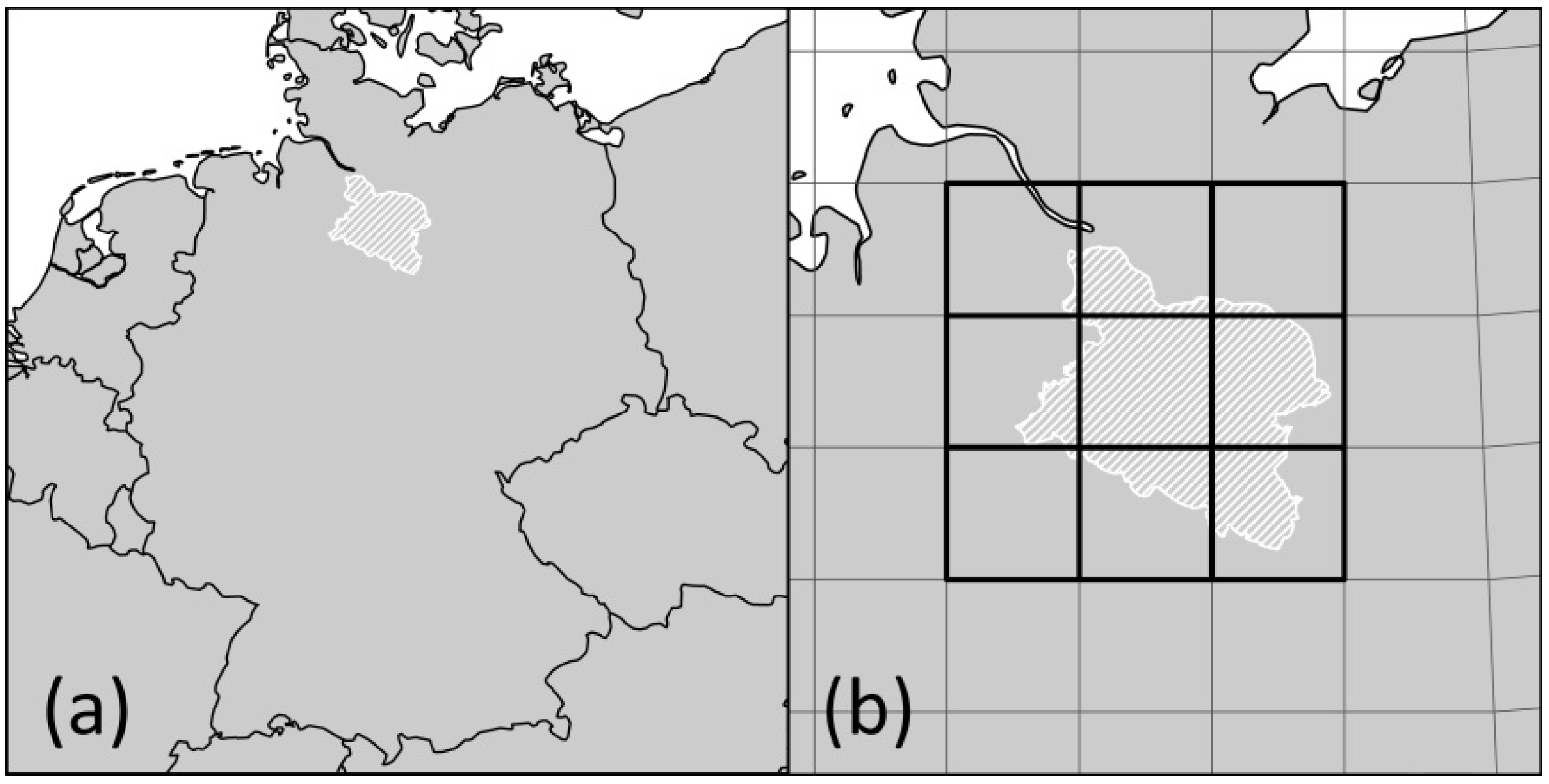
We developed an approach to examine possible turnovers in regional bird communities induced by climate change and applied this approach to assess to what extent climate change might lead to a turnover in the bird community of the Lüneburg Heath region. In addition, we sought to determine which species groups and corresponding habitat types might be most affected in this region. By using species pool comparisons of future climatically analogous regions, we developed an alternative to the widely used bioclimatic envelope models (e.g., [18,46,47]) to assess climate change impacts within a regional context.
The FCAR approach has several advantages. One advantage is that it does not depend on the availability of distribution data for the whole range of the species. In bioclimatic envelope modeling the suitable climate space for species can be underestimated if the complete distribution range of a species cannot be taken into account due to incomplete data or if the range limits of a species are determined by geographical instead of climatic factors. This can lead to an overestimation of local extinctions [48]. Further advantages of the FCAR method are that we are able to include more accurate regional climate projections and that we can take into account the landscape context when assessing climate change impacts.
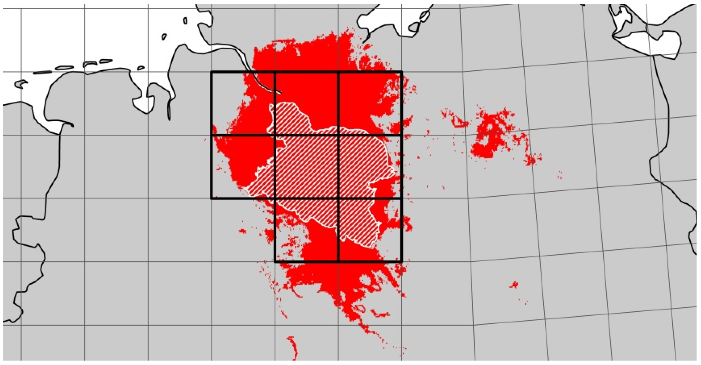
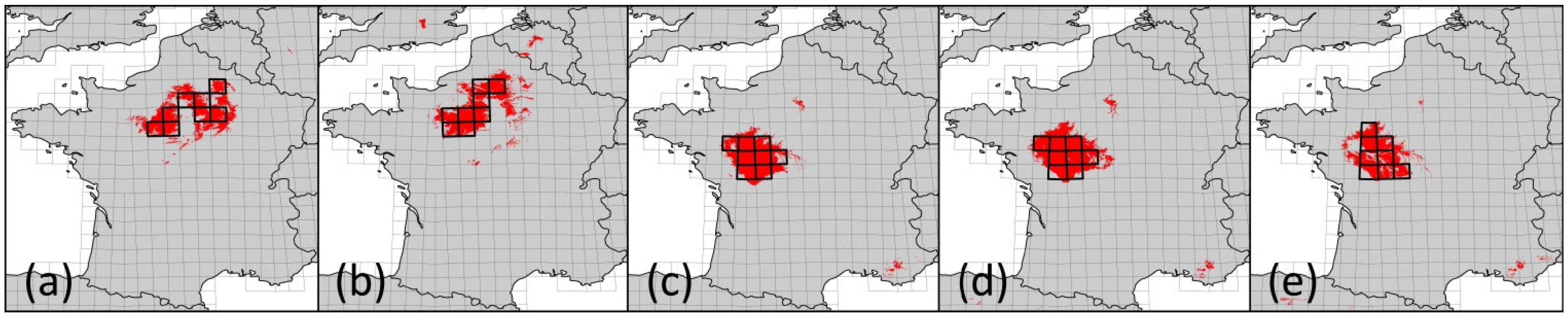
For the LHR we were able to identify four different FCARs representing five different climate projections. However, for two of the altogether seven assessed climate projections, the identified climatically analogous areas were too small to justify species pool comparisons. Thus, when working with an FCAR approach, it is recommendable to use an ensemble of several climate projections because the successful identification of FCARs might not be possible in every case. Further, altitude and land cover have to be sufficiently comparable—as in our study case. However, further research should apply this approach to other regions to test whether it can be transferred to a wide range of regions.
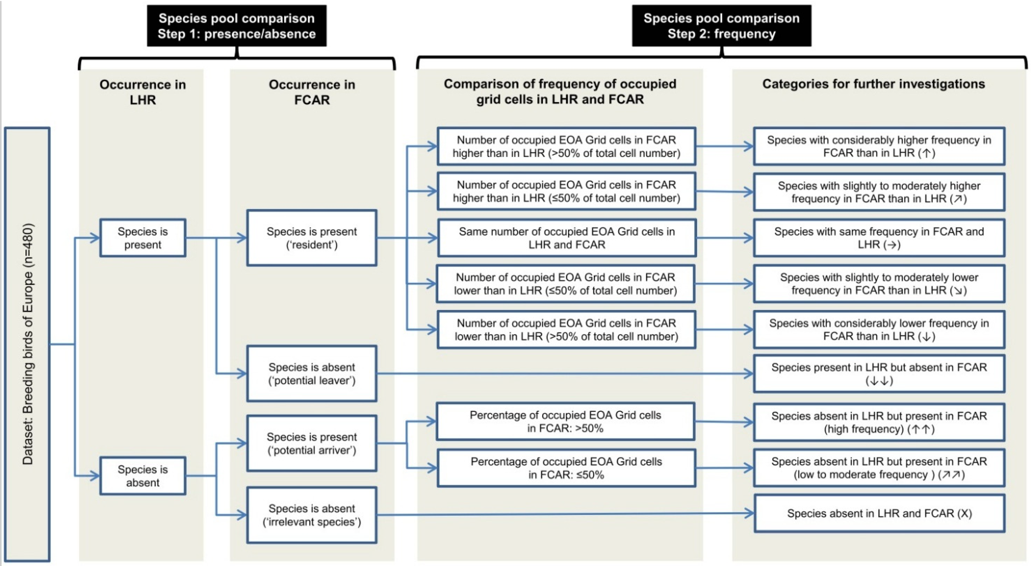
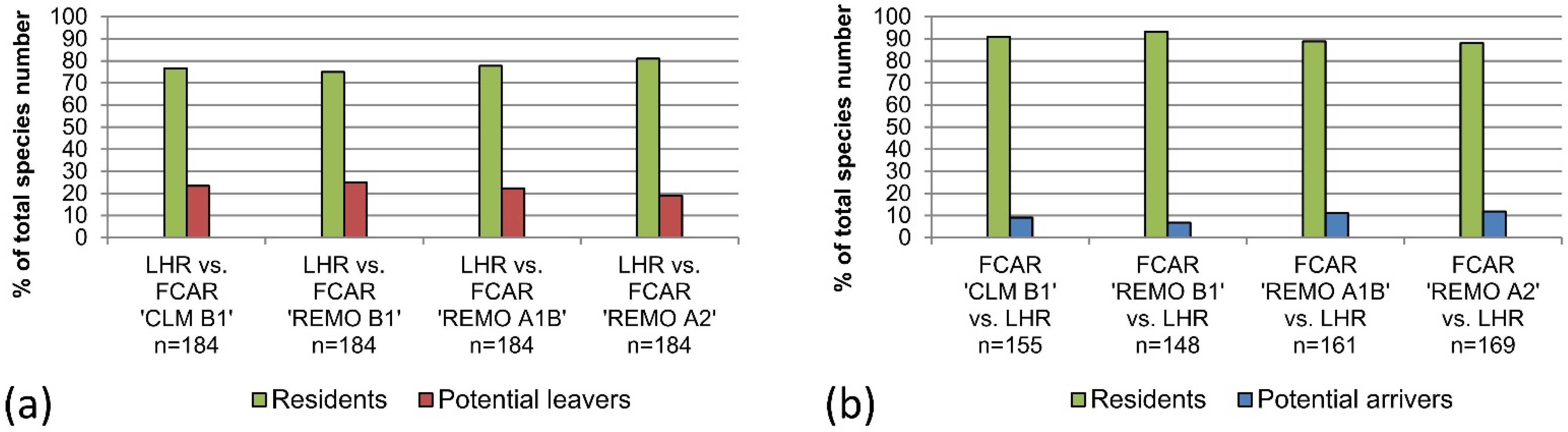
The results of this study indicate that the majority of bird species living in the LHR today would also be able to exist and co-exist in climatic conditions projected for the here considered variables for 2071–2100. However, 19%–25% of today’s LHR-species was categorized as “potential leavers” because they could not be found in the FCARs. The analysis of the data for the LHR from Huntley et al.’s models [
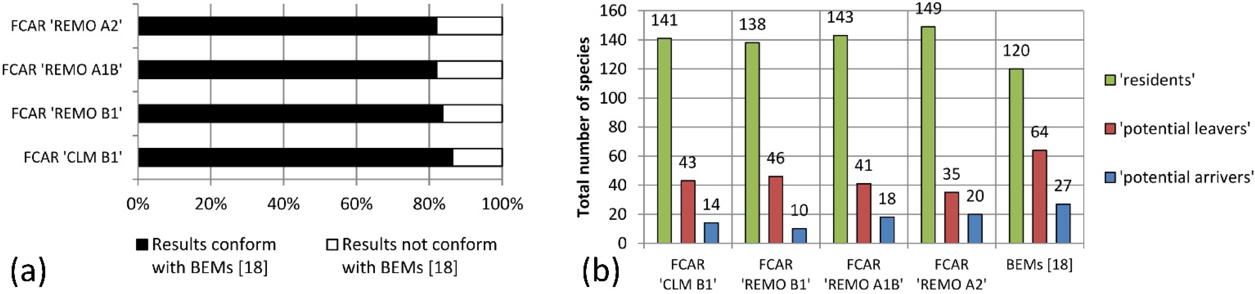
18] show a higher percentage (35%) of “potential leavers.” Both our FCAR approach and the results of Huntley et al. indicate a decrease of bird species diversity for the LHR induced by climatic changes during the 21st century, which is in accordance with other studies (e.g., [49]). In both cases the numbers of “potential leavers” exceeds the number of “potential arrivers.” In general, the degree of conformity of our FCAR approach with the bioclimatic envelope models of Huntley et al. is high for “potential leavers” as well as for “resident” species that have the same or a higher frequency in the FCARs as in the LHR. Interestingly, the degree of conformity is lower for species with a lower frequency of occupied EOA grid cells in the FCARs than in the LHR. Approximately half of the species that we classify as “residents” are absent from the future species pool of the LHR according to Huntley et al. Thus, for the LHR our results show milder impacts than the bioclimatic envelope models of Huntley 
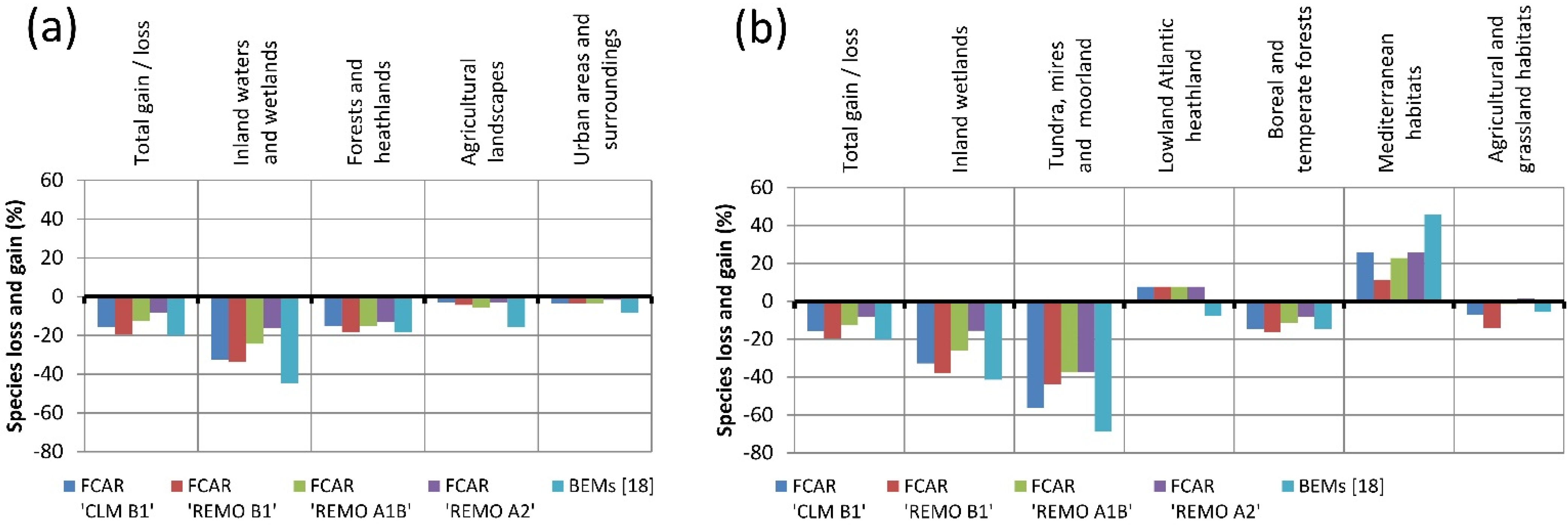
et al., regarding the potential future loss of species. This is especially the case for wetland species. As we found a detectable effect between habitat availability and occurrence in the FCARs for wetland species, it is likely that many of these species can occur in future climates if sufficient habitat is available. Thus, it might be possible that the models of Huntley et al. overestimate the impact of climate change on wetland species in the examined region. In fact, Huntley et al. generally state that the performance of their models was lower for wetland and coastal species. On the other hand, differences between our results and those of Huntley et al. might also be due to differences in the utilized climate models and variables. Our results, however, are based on a wider corridor of climate change models and scenarios.
With the bioclimatic envelope approach by Huntley et al. more “potential arrivers” to the LHR can be identified than with the FCAR approach. We assume that our approach potentially underestimates the number of species that might reach the LHR during the course of climatic changes as the selected EOA grid cells for the species pool comparisons only capture part of the actual climatically analogous area. Other spots in Europe were too small to be included in the species pool comparisons, but might nonetheless function as a source for “potential arrivers.” Additionally, there are recent and historic examples for colonizers from other sources and directions, e.g., the Eurasian Penduline Tit (Remiz pendulinus) and the Fieldfare (Turdus pilaris) coming westwards from Siberia into Europe (for overview see [8]). Further, it was not possible to test if some “potential arrivers” were absent in the FCARs due to habitat conditions.
Despite this underestimation, we wonder how likely it is that “potential arrivers” will actually be able to colonize the study area due to favorable climate conditions. Their colonization potential depends on many factors, including dispersal ability and the status of the source populations. While birds are generally highly mobile and some birds can shift their distribution ranges very rapidly within decades—as documented by Hengeveld [50] for the collared dove (Streptopelia decaocto)—most birds, in contrast, show some degree of site fidelity [8]. In spite of the already documented range shifts (e.g., [4]), there are also studies indicating that birds are currently lagging behind climate warming in their responses [51]. However, the distances that species identified as “potential arrivers” would need to cross to reach the LHR differ greatly. Among the “potential arrivers,” there are species occurring in EOA grid cells adjacent to the LHR and others where the next occurrence is about 700 km away. The median distance of the closest occurrences for all “potential arrivers” is 283 km (see supplementary material—Table S7). Thus, the assessment of the likelihood of “potential arrivers” actually reaching the LHR requires a species-specific interpretation, which is beyond the scope of this study.
Another precondition for “potential arrivers” successfully breeding in the LHR is the availability of suitable habitat. Interestingly, almost half of the “potential arrivers” are or have historically been occasional or regular breeders in Lower Saxony, the federal state the LHR is situated in (see supplementary material—Table S7), showing that this precondition could be met.

4.2. Methodological Limitations

Our approach has some methodological limitations that need to be taken into account when interpreting the results and considering why a species might be present in the LHR, but absent in the FCARs. Some limitations are “data intrinsic.” In order to avoid false absences, we only included EOA grid cells with “good coverage,” meaning that data was provided for at least 75% of the expected breeding species. However, even though this is the atlas’s best survey category, it may be that there is simply no existing data for up to 25% of the species. Furthermore, the data we used is presence/absence data and density was not taken into account. Thus, our approach is limited to assumptions about changes in the distribution of a species because conclusions about population trends within an area are not possible. From a nature conservation point of view, it was important to us to include all species into the analyses, regardless of their frequency within the region. Furthermore, we wanted to use a European-wide data set that does not depend on the availability of regional data. Both aspects imply that the data set therefore in some cases includes occasional breeders or populations of local escapees from captivity that have native populations elsewhere in Europe. We argue that these exceptional cases are of minor importance for assessing trends within a region as we take into account a large assemblage of species.
In our study, we used the climatic variables for our projections that best reflect the distribution of the species community of the LHR. Nonetheless, the effect of other likely important climate variables could not be tested or included because the data was not available. One such climate variable is the incidence of extreme weather events, which are known to pose a risk especially to small populations [52].
Furthermore, there might be other reasons apart from climate for a species to be absent from an area. Concerning land use, a few species that only occur in coastal habitats and not in inland wetlands, might be classified as “potential leavers” due to missing coastal/maritime habitats in the FCARs (e.g., European Herring Gull (Larus argentatus)). However, the percentage of coastal habitats in the LHR is marginal and thus this effect is negligible for the bird community. Furthermore, peat bogs are also missing in the FCARs, but are present in the LHR. In contrast to the sea (and related maritime habitats), which does not depend on climate (cf. [12]), the distribution of peat bogs clearly does (cf. [53]). For species depending on peat bogs we therefore see climate and not land use as the main cause for their absence in the FCARs. Furthermore, we have to consider that species are absent in some cases because of special habitat requirements, which cannot be adequately reflected by the CORINE land cover data. Another source of uncertainty is that not all birds are in equilibrium with the climate within their distribution ranges. Many large raptors, for instance, have a patchy distribution in Europe due to historic or recent persecution [8]. Therefore, when regarding “potential leavers” from a community, assessing a single species requires additional consideration. However, our approach is not designed for making predictions for single species, but for detecting trends within a region.
The method we developed can help to identify species groups that are principally able to cope with the future climatic conditions in a given study area. Nevertheless, climate is not the only factor influencing bird populations within a region and thus occurrence in projected future climates does not automatically mean that a species is not at risk of future declines. Currently, habitat loss and habitat degradation are seen as the major threats to breeding birds in Germany [54]. Hence, species that are already endangered due to land use change have to be monitored carefully, even if they are predicted to occur in future climates. However, Lemoine et al. [55] estimate that climate change has already more influence on population trends of European birds than land use alterations. Additionally, Jiguet et al. [56] found that species with the lowest thermal maxima showed the sharpest declines in Europe recently and Gregory et al. [57] showed that climate change has increasingly impacted European bird populations in the past twenty years.
In our study, we include both migrating and sedentary birds. It is important to keep in mind that migrating birds might additionally be affected by impacts at stop-over and wintering sites. These impacts cannot be included in our approach.
It is necessary to interpret the results of this study cautiously with regards to its limitations. Despite these limitations, we believe the detected overall trends to be a benchmark for estimating future changes in the examined region facing climate change and for developing strategies for nature conservation as the results are based on a range of climate change projections. However, it must not be forgotten that climate change is only one threat to biodiversity and others such as habitat loss and degradation should not be neglected.

4.3. Implications for Nature Conservation

The results from our FCAR approach and the results of the bioclimatic envelope models by Huntley et al. [18] both point in the same direction, indicating that species of inland wetlands might be more impacted by climatic changes than other species groups in this region. However, as we include habitat data in our analyses, we found that climate is not the only important factor determining the occurrence of these species. With our approach we showed that in contrast to species of most other habitat types, the percentage of species of “inland waters and wetlands/inland wetlands” for both of the utilized habitat data sets is significantly positively correlated with the percentage of inland wetlands and inland waters in that area.
Thus, we assume that for the Lüneburg Heath region the extent to which wetland species are affected by climate change can be influenced by the availability and extent of suitable habitat for these species. This is important from a nature conservation point of view, suggesting that more effort in wetland conservation and restoration in the examined region might mitigate climate change impacts on species for these particular habitats.
For future research, testing this approach in other regions and including habitat and species data with a higher resolution is desirable.

Acknowledgments

We wish to thank the EBCC, especially Richard Gregory and Henk Sierdsema, for the provision of the data of the European Breeding Bird Atlas. We also thank Daniel Gerhard for his help with identifying suitable climate variables by performing statistical calculations. Further, we wish to thank Martha Graf and Louise von Falkenhayn for proofreading and commenting on the paper, Christina Weiß and Nana Wix for helpful comments, and René Hertwig, Rüdiger Prasse, and Michael Rode for fruitful discussions. We also thank two anonymous reviewers for their valuable comments.
The study was supported by the Ministry for Science and Culture of Lower Saxony within the network KLIFF—climate impact and adaptation research in Lower Saxony. We acknowledge support by Deutsche Forschungsgemeinschaft and Open Access Publishing Fund of Leibniz Universität Hannover.

Author Contributions

The study was conceived by Janine Sybertz and Michael Reich. Janine Sybertz conducted the study, performed the analyses and interpreted the results with input from Michael Reich. The paper was primarily written by Janine Sybertz with contributions from Michael Reich.

Supplementary Materials

Supplementary materials can be accessed at: https://0-www-mdpi-com.brum.beds.ac.uk/1424-2818/7/1/36/s1.

Conflicts of Interest

The authors declare no conflict of interest.

References

  1. Pulido, F.; Berthold, P. Microevolutionary Response to Climate Change. In Birds and Climate Change; Møller, A.P., Ed.; Elsevier: Amsterdam, The Netherlands, 2004; pp. 151–184. [Google Scholar]
  2. IPCC (Intergovernmental Panel on Climate Change). Climate Change 2007: Synthesis Report. Contribution of Working Groups I, II and III to the Fourth Assessment Report of the Intergovernmental Panel on Climate Change; IPCC: Geneva, Switzerland, 2007. [Google Scholar]
  3. Thomas, C.D.; Lennon, J.J. Birds extend their ranges northwards. Nature 1999, 399, 213. [Google Scholar] [CrossRef]
  4. Parmesan, C.; Yohe, G. A globally coherent fingerprint of climate change impacts across natural systems. Nature 2003, 421, 37–42. [Google Scholar] [CrossRef] [PubMed]
  5. Crick, H.Q.P.; Dudley, C.; Glue, D.E.; Thomson, D.L. UK birds are laying eggs earlier. Nature 1997, 388, 526. [Google Scholar] [CrossRef]
  6. Root, T.L.; Price, J.T.; Hall, K.R.; Schneider, S.H.; Rosenzweig, C.; Pounds, J.A. Fingerprints of global warming on wild animals and plants. Nature 2003, 421, 57–60. [Google Scholar] [CrossRef] [PubMed]
  7. Sparks, T.H.; Bairlein, F.; Bojarinova, J.G.; Hüppop, O.; Lehikoinen, E.A.; Rainos, K.; Sokolov, L.V.; Walker, D. Examining the total arrival distribution of migratory birds. Glob. Chang. Biol. 2005, 11, 22–30. [Google Scholar] [CrossRef]
  8. Newton, I. The Speciation and Biogeography of Birds; Academic Press: London, UK, 2003. [Google Scholar]
  9. Böhning-Gaese, K.; Lemoine, N. Importance of Climate Change for the Ranges, Communities and Conservation of Birds. In Birds and Climate Change; Møller, A.P., Ed.; Elsevier: Amsterdam, The Netherlands, 2004. [Google Scholar]
  10. Luoto, M.; Virkkala, R.; Heikkinen, R.K. The role of land cover in bioclimatic models depends on spatial resolution. Glob. Ecol. Biogeogr. 2007, 16, 34–42. [Google Scholar] [CrossRef]
  11. Araújo, M.B.; Pearson, R.G. Equilibrium of species’ distributions with climate. Ecography 2005, 28, 693–695. [Google Scholar] [CrossRef]
  12. Thuiller, W.; Araújo, M.B.; Lavorel, S. Do we need land-cover data to model species distributions in Europe? J. Biogeogr. 2004, 31, 353–361. [Google Scholar] [CrossRef]
  13. Crick, H.Q.P. The impact of climate change on birds. Ibis 2004, 146, 48–56. [Google Scholar] [CrossRef]
  14. Heikkinen, R.K.; Luoto, M.; Virkkala, R.; Pearson, R.G.; Körber, J.-H. Biotic interactions improve prediction of boreal bird distributions at macro-scales. Glob. Ecol. Biogeogr. 2007, 16, 754–763. [Google Scholar] [CrossRef]
  15. Jiguet, F.; Gadot, A.-S.; Julliard, R.; Newson, S.E.; Couvet, D. Climate envelope, life history traits and the resilience of birds facing global change. Glob. Change Biol. 2007, 13, 1672–1684. [Google Scholar] [CrossRef]
  16. Erasmus, B.F.N.; van Jaarsveld, A.S.; Chown, S.L.; Kshatriya, M.; Wessels, K.J. Vulnerability of South Africa animal taxa to climate change. Glob. Chang. Biol. 2002, 8, 679–693. [Google Scholar] [CrossRef]
  17. Harrison, P.A.; Vanhinsbergh, D.P.; Fuller, R.J.; Berry, P.M. Modelling climate change impacts on the distribution of breeding birds in Britain and Ireland. J. Nat. Conserv. 2003, 11, 31–42. [Google Scholar] [CrossRef]
  18. Huntley, B.; Green, R.E.; Collingham, Y.C.; Willis, S.G. A Climatic Atlas of European Breeding Birds; Lynx: Barcelona, Spain, 2007. [Google Scholar]
  19. Ohlemüller, R.; Gritti, E.S.; Sykes, M.T.; Thomas, C.D. Towards European climate risk surfaces: the extent and distribution of analogous and non-analogous climates 1931–2100. Glob. Ecol. Biogeogr. 2006, 15, 395–405. [Google Scholar] [CrossRef]
  20. Williams, J.W.; Jackson, S.T.; Kutzbach, J.E. Projected distributions of novel and disappearing climates by 2100 AD. Proc. Natl. Acad. Sci. USA 2007, 104, 5738–5742. [Google Scholar] [CrossRef] [PubMed]
  21. Skov, F.; Nygaard, B.; Wind, P.; Borchsenius, F.; Normand, S.; Balslev, H.; Fløjgaard, C.; Svenning, J.-C. Impacts of 21st century climate changes on flora and vegetation in Denmark. IOP Conf. Ser.: Earth Environ. Sci. 2009, 8, 1–13. [Google Scholar] [CrossRef]
  22. Bergmann, J.; Pompe, S.; Ohlemüller, R.; Freiberg, M.; Klotz, S.; Kühn, I. The Iberian Peninsula as a potential source for the plant species pool in Germany under projected climate change. Plant Ecol. 2009, 207, 191–201. [Google Scholar] [CrossRef]
  23. Huntley, B. European post-glacial forests: Compositional changes in response to climatic change. J. Veg. Sci. 1990, 1, 507–518. [Google Scholar] [CrossRef]
  24. Olesen, J.E.; Bindi, M. Consequences of climate change for European agricultural productivity, land use and policy. Eur. J. Agron. 2002, 16, 239–262. [Google Scholar] [CrossRef]
  25. NLWKN (Niedersächsischer Betrieb für Wasserwirtschaft, Küsten- und Naturschutz). NATURA 2000: Europäische Vogelschutzgebiete und gemeldete FFH-Gebiete in Niedersachsen. Shape Files. Available online: http://www.umwelt.niedersachsen.de/portal/live.php?navigation_id=2540&article_id=9124&_psmand=10 (accessed on 14 April 2009).
  26. Müller, T. 64 Lüneburger Heide. In Handbuch der naturräumlichen Gliederung Deutschlands; 7. Lieferung, Bd. 2; Meynen, E., Schmithüsen, J., Gellert, J.F., Neef, E., Müller-Miny, H., Schultze, J.H., Eds.; Veröffentlichungen des Instituts für Landeskunde und des deutschen Instituts für Länderkunde (Bundesanstalt für Landeskunde und Raumforschung): Bad Godesberg, Germany, 1965; pp. 959–964. (In German) [Google Scholar]
  27. Von Drachenfels, O. Überarbeitung der Naturräumlichen Regionen Niedersachsens. Inf.dienst Nat.schutz Niedersachs. 2010, 4, 249–252. (In German) [Google Scholar]
  28. The EBCC Atlas of European Breeding Birds: Their Distribution and Abundance; Hagemeijer, E.J.M.; Blair, M.J. (Eds.) T & A.D. Poyser: London, UK, 1997.
  29. Hijmans, R.J.; Cameron, S.E.; Parra, J.L.; Jones, P.G.; Jarvis, A. Very high resolution interpolated climate surfaces for global land areas. Int. J. Climatol. 2005, 25, 1965–1978. [Google Scholar] [CrossRef]
  30. Keuler, K.; Lautenschlager, M.; Wunram, C.; Keup-Thiel, E.; Schubert, M.; Will, A.; Rockel, B.; Boehm, U. Climate Simulation with CLM, Scenario B1 Run no.1, Data Stream 2: European Region MPI-M/MaD, 2009, World Data Center for Climate. Available online: http://cera-www.dkrz.de/WDCC/ui/EntryList.jsp?acronym=CLM_B1_1_D2 (accessed on 9 June 2011).
  31. Jacob, D. REMO B1 Scenario Run, UBA Project, 0.088 Degree Resolution, Run no. 006212, 1H Data, 2005, World Data Center for Climate, CERA-DB “REMO_UBA_B1_1_R006212_1H”. Available online: http://cera-www.dkrz.de/WDCC/ui/Compact.jsp?acronym=REMO_UBA_B1_1_R006212_1H (accessed on 20 May 2011).
  32. Keuler, K.; Lautenschlager, M.; Wunram, C.; Keup-Thiel, E.; Schubert, M.; Will, A.; Rockel, B.; Boehm, U. Climate Simulation with CLM, Scenario A1B Run no.1, Data Stream 2: European Region MPI-M/MaD, 2009, World Data Center for Climate. Available online: http://cera-www.dkrz.de/WDCC/ui/EntryList.jsp?acronym=CLM_A1B_1_D2 (accessed on 16 April 2010).
  33. Keuler, K.; Lautenschlager, M.; Wunram, C.; Keup-Thiel, E.; Schubert, M.; Will, A.; Rockel, B.; Boehm, U. Climate Simulation with CLM, Scenario A1B Run no.2, Data Stream 2: European Region MPI-M/MaD, 2009, World Data Center for Climate. Available online: http://cera-www.dkrz.de/WDCC/ui/EntryList.jsp?acronym=CLM_A1B_2_D2 (accessed on 27 April 2010).
  34. Jacob, D. REMO A1B Scenario Run, UBA Project, 0.088 Degree Resolution, Run no. 006211, 1H Data, 2005, World Data Center for Climate, CERA-DB “REMO_UBA_A1B_1_R006211_1H”. Available online: http://cera-www.dkrz.de/WDCC/ui/Compact.jsp?acronym=REMO_UBA_A1B_1_R006211_1H (accessed on 15 April 2010).
  35. Jacob, D.; Nilson, E.; Tomassini, L.; Bülow, K. REMO A1B Scenario Run, BFG Project, 0.088 Degree Resolution, 1H Values, 2009, World Data Center for Climate, CERA-DB “REMO_BFG_A1B_1H”. Available online: http://cera-www.dkrz.de/WDCC/ui/Compact.jsp?acronym=REMO_BFG_A1B_1H (accessed on 7 April 2010).
  36. Jacob, D. REMO A2 Scenario Run, UBA Project, 0.088 Degree Resolution, Run no. 006213, 1H Data, 2005, World Data Center for Climate, CERA-DB “REMO_UBA_A2_1_R006213_1H”. Available online: http://cera-www.dkrz.de/WDCC/ui/Compact.jsp?acronym=REMO_UBA_A2_1_R006213_1H (accessed on 20 May 2011).
  37. Jacob, D. REMO Climate of the 20th Century Run, UBA Project, 0.088 Degree Resolution, Run no. 006210, 1H Data, 2005, World Data Center for Climate, CERA-DB “REMO_UBA_C20_1_R006210_1H”. Available online: http://cera-www.dkrz.de/WDCC/ui/Compact.jsp?acronym=REMO_UBA_C20_1_R006210_1H (accessed on 15 April 2010).
  38. Jacob, D.; Nilson, E.; Tomassini, L.; Bülow, K. REMO Climate of the 20th Century Run, BFG Project, 0.088 Degree Resolution, Run no. 2, 1H Data, 2009, World Data Center for Climate, CERA-DB “REMO_BFG_C20_1H”. Available online: http://cera-www.dkrz.de/WDCC/ui/Compact.jsp?acronym=REMO_BFG_C20_1H (accessed on 7 April 2010).
  39. Keuler, K.; Lautenschlager, M.; Wunram, C.; Keup-Thiel, E.; Schubert, M.; Will, A.; Rockel, B.; Boehm, U. Climate Simulation with CLM, Climate of the 20th Century run no.2, Data Stream 2: European Region MPI-M/MaD, 2009, World Data Center for Climate. Available online: http://cera-www.dkrz.de/WDCC/ui/EntryList.jsp?acronym=CLM_C20_2_D2 (accessed on 7 April 2010).
  40. Lautenschlager, M.; Keuler, K.; Wunram, C.; Keup-Thiel, E.; Schubert, M.; Will, A.; Rockel, B.; Boehm, U. Climate Simulation with CLM, Climate of the 20th Century Run no.1, Data Stream 2: European Region MPI-M/MaD, 2009, World Data Center for Climate. Available online: http://cera-www.dkrz.de/WDCC/ui/EntryList.jsp?acronym=CLM_C20_1_D2 (accessed on 6 April 2010).
  41. EEA (European Environment Agency). Corine Land Cover 2006 Raster Data—Version 13 (02/2010). Available online: http://www.eea.europa.eu/data-and-maps/data/corine-land-cover-2006-raster (accessed on 17 May 2011).
  42. Schröder, K.; Schikore, T.; Andretzke, H. Hinweise auf Lebensraum bezogene Erfassungen. In Methodenstandards zur Erfassung der Brutvögel Deutschlands; Südbeck, P., Andretzke, H., Fischer, S., Gedeon, K., Schikore, T., Schröder, K., Sudfeldt, C., Eds.; Länderarbeitsgemeinschaft der Vogelschutzwarten und Dachverband Deutscher Avifaunisten e. V.: Radolfzell, Germany, 2005; pp. 114–134. (In German) [Google Scholar]
  43. Tucker, G.M.; Evans, M.I. Habitats for Birds in Europe. A Conservation Strategy for the Wider Environment; Birdlife International: Cambridge, UK, 1997. [Google Scholar]
  44. Bird Life International. Birds in Europe: Population Estimates, Trends and Conservation Status; Bird Life International: Cambridge, UK, 2004. [Google Scholar]
  45. R Development Core Team. R: A Language and Environment for Statistical Computing; R Foundation for Statistical Computing: Vienna, Austria, 2008. [Google Scholar]
  46. Araújo, M.B.; Thuiller, W.; Pearson, R.G. Climate warming and the decline of amphibians and reptiles in Europe. J. Biogeogr. 2006, 33, 1712–1728. [Google Scholar] [CrossRef]
  47. Settele, J.; Kudrna, O.; Harpke, A.; Kühn, I.; van Swaay, C.; Verovnik, R.; Warren, M.; Wiemers, M.; Hanspach, J.; Hickler, T.; et al. Climatic Risk Atlas of European Butterflies; Pensoft: Sofia, Bulgaria, 2008. [Google Scholar]
  48. Barbet-Massin, M.; Thuiller, W.; Jiguet, F. How much do we overestimate future local extinction rates when restricting the range of occurrence data in climate suitability models? Ecography 2010, 33, 878–886. [Google Scholar] [CrossRef]
  49. Barbet-Massin, M.; Thuiller, W.; Jiguet, F. The fate of European breeding birds under climate, land-use and dispersal scenarios. Glob. Change Biol. 2012, 18, 881–890. [Google Scholar] [CrossRef]
  50. Hengeveld, R. Mechanisms of biological invasions. J. Biogeogr. 1988, 15, 819–828. [Google Scholar] [CrossRef]
  51. Devictor, V.; Julliard, R.; Couvet, D.; Jiguet, F. Birds are tracking climate warming, but not fast enough. Proc. R. Soc. B 2008, 275, 2743–2748. [Google Scholar] [CrossRef] [PubMed]
  52. Primack, R. A Primer of Conservation Biology, 4th ed.; Sinauer Associates: Sunderland, MA, USA, 2008. [Google Scholar]
  53. Lottes, A.L.; Ziegler, A.M. World peat occurrence and the seasonality of climate and vegetation. Palaeogeogr. Palaeoclimatol. Palaeoecol. 1994, 1006, 23–37. [Google Scholar] [CrossRef]
  54. Südbeck, P.; Bauer, H.-G.; Boschert, M.; Boye, P.; Knief, W. Rote Liste der Brutvögel Deutschlands (The red list of breeding birds of Germany). Ber. Vogelschutz 2007, 44, 23–81. (In German) [Google Scholar]
  55. Lemoine, N.; Bauer, H.-G.; Peintinger, M.; Böhning-Gaese, K. Effects of Climate and Land-Use Change on Species Abundance in a Central European Bird Community. Conserv. Biol. 2007, 21, 495–503. [Google Scholar] [CrossRef] [PubMed]
  56. Jiguet, F.; Gregory, R.D.; Devictor, V.; Green, R.E.; Voříšek, P.; van Strien, A.; Couvet, D. Population trends of European common birds are predicted by characteristics of their climatic niche. Glob. Chang. Biol. 2010, 16, 497–505. [Google Scholar] [CrossRef]
  57. Gregory, R.D.; Willis, S.G.; Jiguet, F.; Voříšek, P.; Klvaňová, A.; van Strien, A.; Huntley, B.; Collingham, Y.C.; Couvet, D.; Green, R.E. An Indicator of the Impact of Climatic Change on European Bird Populations. PLoS One 2009, 4, e4678:1–e4678:6. [Google Scholar] [CrossRef] [Green Version]

