Application of Rough Set Theory to Water Quality Analysis: A Case Study

Abstract

This work proposes an approach to analyze water quality data that is based on rough set theory. Six major water quality indicators (temperature, pH, dissolved oxygen, turbidity, specific conductivity, and nitrate concentration) were collected at the outlet of the watershed that contains the George Mason University campus in Fairfax, VA during three years (October 2015–December 2017). Rough set theory is applied to monthly averages of the collected data to estimate one indicator (decision attribute) based on the remainder indicators and to determine what indicators (conditional attributes) are essential (core) to predict the missing indicator. The redundant attributes are identified, the importance degree of each attribute is quantified, and the certainty and coverage of any detected rule(s) is evaluated. Possible decision making rules are also assessed and the certainty coverage factor is calculated. Results show that the core water quality indicators for the Mason watershed during the study period are turbidity and specific conductivity. Particularly, if pH is chosen as a decision attribute, the importance degree of turbidity is higher than the one of conductivity. If the decision attribute is turbidity, the only indispensable attribute is specific conductivity and if specific conductivity is the decision attribute, the indispensable attribute beside turbidity is temperature.

1. Introduction

Since water quality is affected by complex factors like animal/human activities and weather events, its continuous sampling and monitoring is of paramount importance for human health [1]. The United States Geological Survey (USGS) has been continuously monitoring the quality of surface water across the U.S. over the past decades [2]. The most common water quality indicators suggested by the USGS are temperature, specific conductance, dissolved oxygen concentration (DO), pH, and turbidity. Collecting and analyzing water quality data is a challenging task. First off, water quality monitoring techniques are different in different water bodies like streams, lakes, bays, and estuaries, characterized not only by different microscopic and macroscopic organisms, but also by different ecosystems, flow rate, and accessibility. Additional common challenges include uncertainty in water quality observations and instrument failure. In the instance of instrument malfunctioning or stop recording, one or more values in the time series may be missing. Popular methods to recover gaps in time series are divided into two major groups: deterministic and stochastic [3]. Examples of deterministic approaches are nearest-neighbor interpolation, polynomial interpolation, and methods based on distance weighting. Regression methods, auto regressive methods, and machine learning methods fall under the stochastic category [3].

Sampling water quality is further complicated by the development of an effective method to analyze and evaluate the collected data. Water quality data are usually characterized by non-Gaussian distributions. Also, the presence of outliers and missing values are very common [4]. As a result, finding an appropriate analytical method is key. Some popular classical methods are graphical analysis (e.g., boxplots, scatter plots, and Q-Q plots), probability distribution analysis, and trend analysis. However, when dealing with excessive amount of data, it is easy to miss hidden patterns and information. In the past two decades, several studies have proposed novel approaches to analyze water quality data, including fuzzy theory [5], maximum likelihood methods [6], principal component analysis [7], cascade correlation artificial neural network [8], interactive fuzzy multi-objective linear programming [9], linear regression [10], inexact chance-constrained quadratic programming [11], and Dempster-Shafer methods [12]. All these methods have the ability to deal with large datasets and investigate relationships among water quality indicators. However, to take advantage of the above tools, prior and/or additional information about the data is needed. For example, the fuzzy set theory requires a grade of membership (that defines how each data point is mapped to a membership value) or a value of possibility (e.g., possible, quite possible, slightly possible, impossible). Similarly, the Dempster-Shafer theory necessitates basic probability analysis [13].

Rough Set Theory (RST), introduced by Pawlak in 1982 [13], represents a valid alternative to overcome these issues. RST is a powerful tool to deal with large amounts of information, does not require preliminary or additional information about the data, and considers vagueness and uncertainty in the dataset [14]. RST is commonly used in classification, ranking, multi-criteria decision analysis, and decision rules [15]. One of the applications of RST is pattern recognition by attribute reduction. By reducing unnecessary features, RST is capable of discovering hidden patterns in high dimensional datasets [16]. The philosophy of rough set is based on the assumption that some information is associated to every object in the universe. Objects sharing the same information are called indiscernible and the indiscernibility relation is the mathematical basis of rough set theory [17]. This tool has been successfully applied to areas like healthcare, banking, medicine, engineering, environmental science, among others [17].

In this work, we investigate the potential of applying RST to water quality analysis. RST is useful when dealing with complexity and vagueness in a dataset, which is always the case when analyzing water quality field data. Although a few attempts exist in the field of environmental and water resources engineering [18,19], the application of RST for assessing water quality indicators has not been widely explored. For example, Shen and Chouchoulas [20] proposed a hybrid system called fuzzy-rough estimator to assess the size of algae population based on water characteristics. Although their attribute reduction method (going from eleven original attributes to seven) was demonstrated to be successful, their approach was not capable of extracting high accuracy sets of rules. Another application of RST in water resources engineering is the one investigated by Barbagallo et al. [21] who studied reservoir operating rules. This study employed the integrated RST and Rose application, a software developed by the University of Poznan in Poland [22], to provide the minimal condition attributes and reveal the relevance of each attribute. Dong et al. [18] proposed a model to forecast annual runoff from a reservoir using RST. Their results showed that the larger the samples was, the more accurate the model. In a study performed by Ip et al. [23], RST was employed to identify the significant water quality indicators in a decision-making system. Specifically, RST was able to reduce the number water quality indicators and quantify the importance degree of each core indicator.

Other studies combined RTS with other approaches, such as the one by Pai and Lee [19] that introduced the Multinomial Logistics Regression (MLR) model. MLR was used to investigate the relationship between different degrees of water pollution and environmental factors, like the one between the concentration of SO₂ emitted by car and motorcycle exhausts and ozone density in the atmosphere. This framework was shown to be capable of predicting water quality using environmental factors rather than monitoring the processes of chemical elements. Another example is the work by Karimi et al. [24] who employed the variable consistency dominance-based rough set approach to explore the complex relationship between water quality and environmental indicators. They explored the relationship between total dissolved solids (TDS) and environmental indicators used as explanatory variables, such as precipitation, river water temperature, runoff, normalized difference vegetation index (NVDI), land surface temperature, river water temperature. Using a moving average filter in the TDS data, they decreased the noise and reduced the width of the boundary region between the lower approximation (all elements in a subset belong to the set) and upper approximation (all elements possibly belong to the set).

The main goal of this work is to assess the efficiency of using RST to estimate one water quality indicator based on given (known) indicators. Evaluating the overall quality of the stream water is outside the scope of this work. What we consider here is a comprehensive approach that looks at several water quality indicators rather than providing a generic assessment of the stream healthiness. Our hypothesis is that, when observations in a time series are missing, RST is capable of providing information regarding the missing indicator based on the other recorded indicators. RST also identifies the dispensable indicators. By eliminating the dispensable (redundant) indicator or indicators, the complexity of the dataset is reduced. The strength of each indicator in finding an unknown indicator is assessed and dispensable attributes are identified to discover hidden patterns. Section 2 introduces the basics of rough set theory and its application to a water quality dataset collected in Fairfax, VA during 2015 to 2017. Section 3 presents the results, whereas Section 4 discusses the results and summarizes the main conclusions.

2. Materials and Methods

2.1. Rough Set Theory

In RST, data are represented by an information system or information table consisting of non-empty sets of finite objects (rows) and non-empty finite set of attribute (columns). More formally:

S = (U, A)

(1)

where S is the decision system, U is the universe, and A is an attribute.

The central concept in RST is the indiscernibility relation, a relationship between two (or more) objects where all the values are identical (equivalent) with respect to a subset of considered attributes [25]. The indiscernibility relation is defined as any subset B of A with a binary relation I (B) on U. For every a ∈ A: (x, y) ∈ I(B) if and only if a(x) = a(y), where the value of attribute a is for element x (or y).

Approximation is another fundamental concept in RST. On one hand, lower approximation refers to the domain of objects that are known with certainty to belong to the subset of interest. The lower approximation is also called B-positive region, posB(X). On the other hand, upper approximation refers to objects that possibly belong to the subset of interest [26].

Suppose X ⊂ U, and B ⊂ A, the B_lower and B_upper approximation of X, respectively, are:

B_lower (X) = ∪ {B(x):B(x) ⊂ X}

(2)

B_upper (X) = ∪ {B(x):B(x) ∩ X ≠ ∅}.

(3)

Therefore, the B-boundary region of X is defined as:

BNB(X) = B_upper (X) − B_lower (X).

(4)

If the boundary region is empty, then X is exact (or crisp). Otherwise, X is inexact and is classified as rough. The approximation method is a valuable method to express data topological properties [14]. The decision-making (DM) rule is another helpful tool to discover hidden patterns in a dataset and is defined as follows:

S = (U, C, D)

(5)

where C is a disjoint set of condition attributes and D is the decision attribute. For every x ⊂ U, there exist C1(x), …, Cn(x), d1(x), …, dm(x). The decision rule induced by x in S is:

C1(x), …, Cn(x) → d1(x), …, dm(x) or C →D.

(6)

where the arrow implies the decision D is based on condition C. The importance degree of attributes relative to the decision is calculated as:

γcd (c) = {|posc(D)|/|U|} − {|pos(c − {c})(D)|/|U|}.

(7)

This way the most important attributes are selected and if the importance degree equals zero, the attribute is unimportant. The larger γcd (c), the higher the attribute degree of importance is. Please note that the importance degree is not a percentage and has no units. If |x| is the number of element in a set (i.e., cardinality of x), then the support of decision is defined as:

suppx(C,D) = |A(x)| = |C(x) ∩ D(x)|

(8)

and the strength of the decision is quantified as:

σx(C,D) = suppx(C,D)/|U|.

(9)

In other words, the support of the decision corresponds to the number of times that a certain rule is observed within the dataset and the strength of the decision is the support of the decision divided by the total number of decision rules. So, if the support of a decision is high, it means that the number of times that the specific decision rule is repeated is high and consequently, this decision rule is strong.

Also, the certainty of the decision rule is calculated as:

cerx(C,D) = [|C(x) ∩ D(x)|]/|C(x)| = suppx(C,D)/|C(x)| = σx(C,D)/π|C(x)|

(10)

where π|C(x)| = |C(x)|/|U|. When cerx equals to one, then C→xD is a certain decision rule.

Another useful factor in the DM rule concept is the coverage of decision rule defined as:

covx(C,D) = [|C(x) ∩ D(x)|]/|D(x)| = suppx(C,D)/|D(x)| = σx(C,D)/π|D(x)|

(11)

where π|C(x)| = |D(x)|/|U|. The coverage coefficient is the conditional probability of reasons for a given decision.

When C→xD is a decision rule, then D→xC is called the inverse decision rule and can be used to give explanations (reasons) for a decision. Please note that the certainty factors for inverse decision rules are coverage factors for the original decision rule [14].

2.2. Study Area and Dataset

In this study, we evaluate the chemical and physical quality of water at the outlet of the watershed that contains the George Mason University campus in Fairfax, VA. Figure 1 shows the watershed boundaries and the location where water quality indicators were sampled. This urbanized watershed contains two small creeks and one retention pond and is located within the larger Pohick Creek Watershed. Moreover, it consists of generally flat to sloping topography with most drainage (approximately 90%) flowing towards the south central portion of the campus and Pohick Creek.

A water quality monitoring instrument (the Eureka Manta2 Waterprobe) with six sensors automatically records six water quality indicators (listed in

Table 1. Units, average, standard deviation, 25th and 75th quartiles of water quality indicators collected during the study period at the location shown in Figure 1.

	Dissolved Oxygen	Nitrate Concentration	Specific Conductivity	Temperature	Turbidity	pH
Symbol	DO	NO3	K	T	Tu	pH
Units	mg/L	mg/L	uS/cm	°C	NTU	-
Average	6.14	136	342	20.7	40.9	6.75
St. Deviation	1.23	46.4	126	3.63	95.7	0.16
25th Quartile	5.58	128	280	18.4	5.67	6.65
75th Quartile	6.72	158	384	23.3	36	6.82

): dissolved oxygen concentration (DO), nitrate concentration, pH, specific conductivity, temperature, and turbidity. These water quality indicators were chosen for several reasons. First off, they are listed by the Environmental Protection Agency (EPA) to define water quality standards for surface water [27]. Secondly, since George Mason University complies with the Clean Water Act and EPA storm water regulations, its Facilities Department monitors these indicators across the campus every year [28]. The water quality probe recorded each indicator every hour from October 2015 to December 2017. However, the probe was out for calibration and repairs occasionally and there have been some frequent network issues with the data logger. As a result, only 14 months of data are used in this work.

Most data have been collected during 2016 and 2017. Both years are characterized by monthly mean temperature and precipitation that are similar to the 30-year mean values for the region [29]. Specifically, the average temperature during the past 30-year in Fairfax, VA is 13 °C and the yearly average temperature both in 2016 and 2017 is 14 °C. The average 30-year cumulative precipitation is 107 cm and the average precipitation for 2016 and 2017 is 90 cm and 104 cm, respectively. This indicates that 2016 and 2017 are not anomalous years in terms of regional climatology [29]. The collected data, summarized in Table 1, show that water temperature fluctuates from about 5 °C in winter to almost 30 °C in summer. The average pH is 6.75 and it falls in the range identified by EPA water quality standards for the Commonwealth of Virginia [27]. The average DO is 6.14 mg/L and it is also within the EPA water quality standards. The level of nitrate (average of 136.11 mg/L-N) shows that the runoff water possibly traveled through lands with fertilizers. Another possible source of nitrate is the atmosphere containing nitrogen compounds derived from automobiles [30]. According to EPA, the natural level of nitrate from wastewater effluent can range up to 30 mg/L. Finally, the high standard deviations in conductivity and turbidity are also common because of the frequent storms in this region.

The collected data are then discretized into three categories (low, medium and high): (i) any value lower than the 25th quartile is classified as low (L); (ii) any value between the 25th and 75th quartiles is classified as medium (M); and (iii) any value higher than the 75th quartile is classified as high (H).

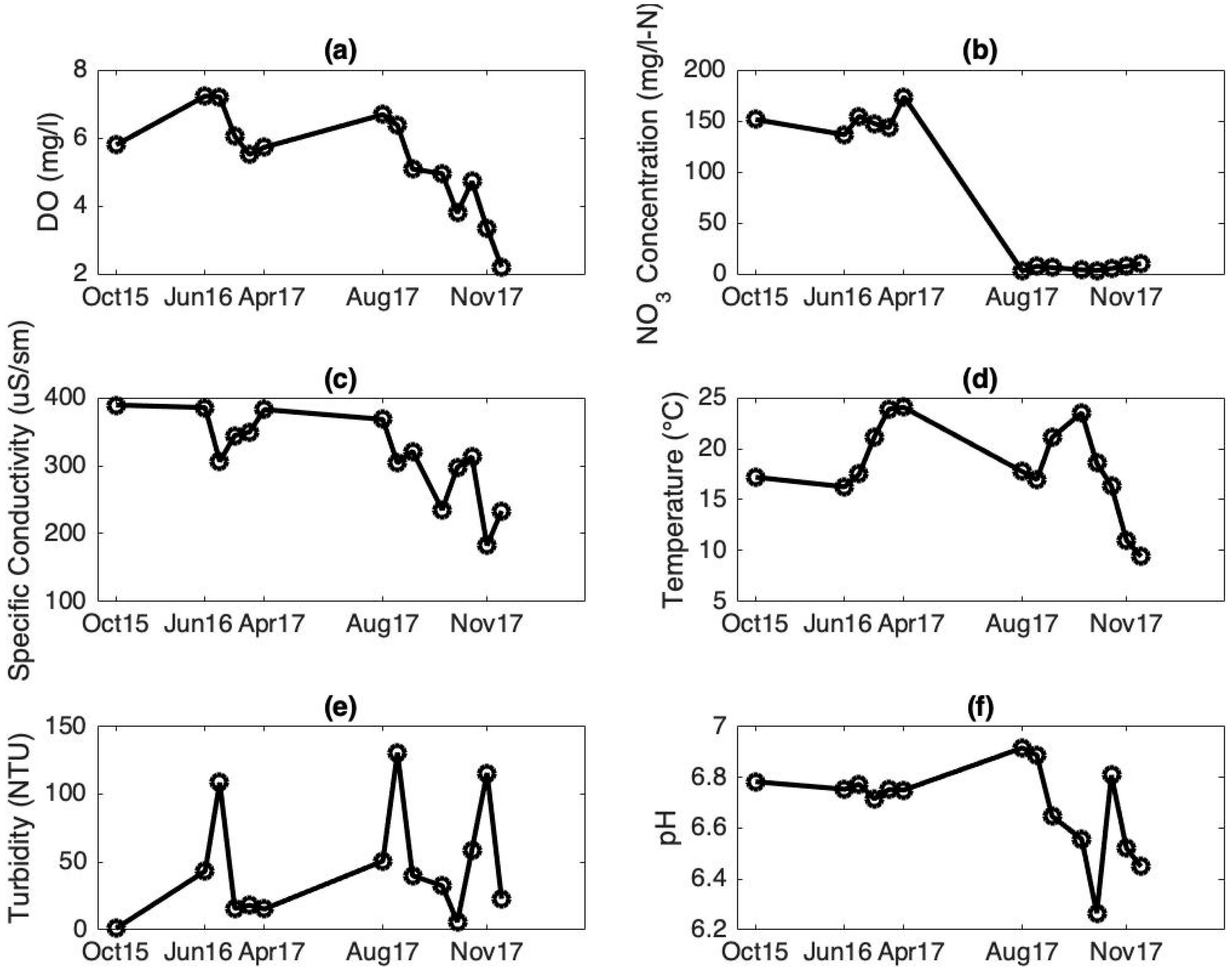
A plot of time series of all the water quality indicators during the study period is shown in Figure 2. The inverse correlation between pH and temperature is clearly notable. However, it is important to mention that correlations between water quality indicators (as shown in [31]) at monthly scales are affected by several parameters, including environmental conditions and anthropogenic factors (e.g., rainfall events, construction sites).

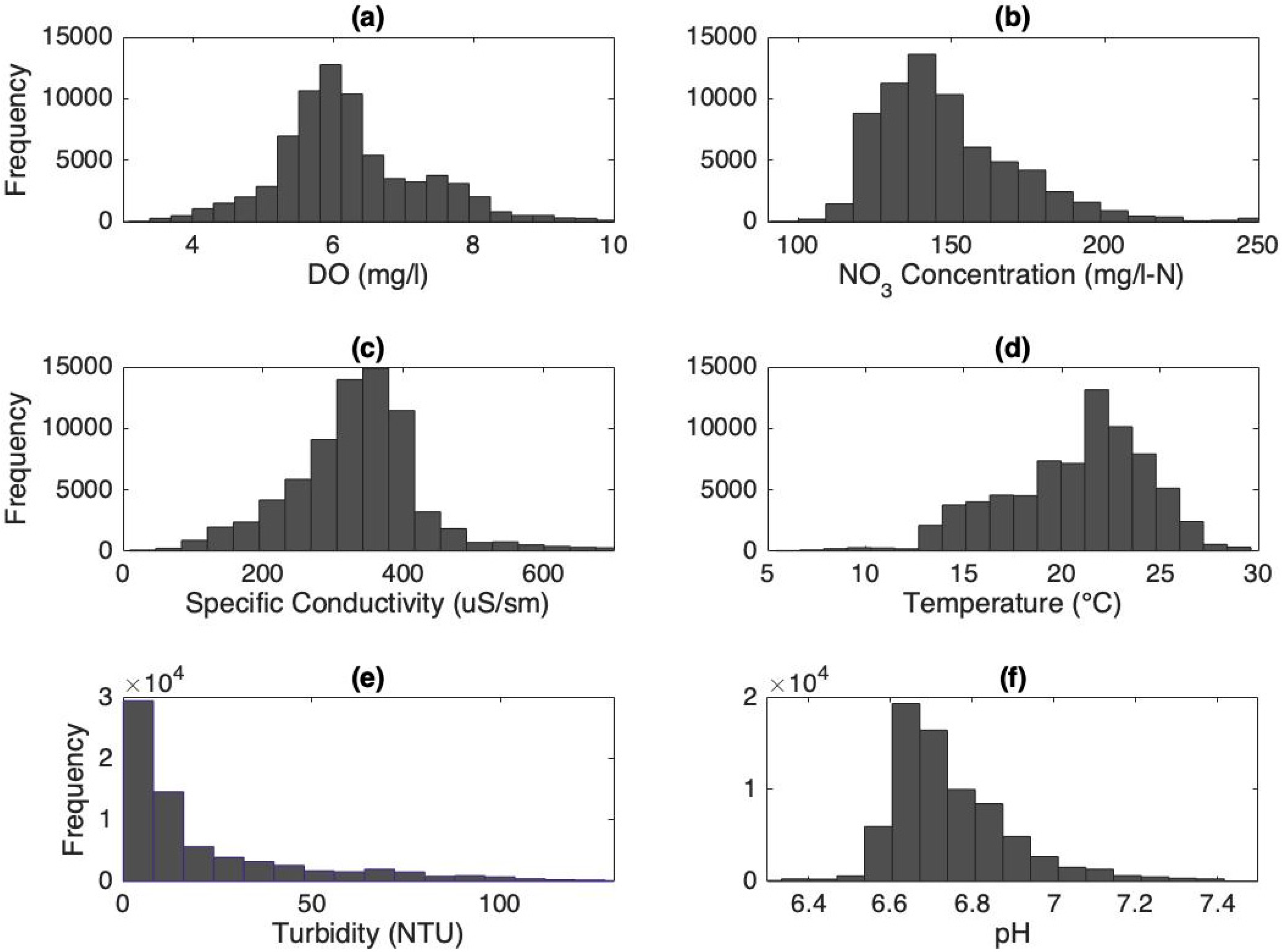
The shape of the frequency distributions for the water quality indicators considered in this study demonstrates the difficulty of fitting a known distribution to these datasets (Figure 3). For instance, the turbidity frequency distribution—shown in Figure 3e—is clearly non-normal and skewed towards lower values, with a long tail at higher values. On the other hand, some indicators (e.g., DO, specific conductivity) show more symmetrical distributions.

3. Results

The information table is set up to apply RST to the data collected at the Mason watershed outlet. Specifically, five water quality indicators are chosen as the conditional attributes and the sixth one as the decision attribute. The water quality probe reads each water quality indicator every hour. However, in order to introduce rough set theory to water quality analysis, coarse resolution (monthly average) data are examined. This not only helps with showing a limited amount of condition and decision attributes in the following tables, but also helps to reduce the random noise in the data sample. Numerical values are assigned to each of the 14 months and presented as time codes in

Table 2. Attributes and decision values where pH is the decision attributes and the other indicators are condition attributes.

Time Code	Date (M-Y)	DO	NO3	K	T	Tu	pH
1	October-15	M	M	H	L	L	M
2	April-16	H	M	H	L	H	M
3	May-16	H	M	M	L	H	M
4	June-16	M	M	M	M	M	M
5	July-16	L	M	M	H	M	M
6	August-16	M	H	M	H	M	M
7	April-17	M	L	M	L	H	H
8	May-17	M	L	M	L	H	H
9	June-17	L	L	M	M	H	L
10	August-17	L	L	L	H	M	L
11	September-17	L	L	M	M	M	L
12	October-17	L	L	M	L	H	M
13	November-17	L	L	L	L	H	L
14	December-17	L	L	L	L	M	L

. The following analysis is based on the scenario in which pH is chosen as the decision attribute (D) and the rest of the indicators as condition attributes (C). In set theory formalism, this corresponds to U = {1, 2, 3, 4, 5, 6, 7, 8, 9, 10, 11, 12, 13, 14}, C = {DO, NO₃, K, T, Tu}, and D = {pH}, where C and D can be either L, or M, or H.

The first step is to identify redundant (or identical) time codes. After analyzing each time code, {7} and {8} are the only ones found identical, not only in terms of attributes, but also in terms of decision. This means that every single conditional and decision attribute is the same for time codes {7} and {8}. The fact that they are identical not only in terms of condition attributes but also in terms of decision attributes shows that if DO and K are medium, NO₃ and T are low, and Tu is high, pH is certainly high. This is the first certain decision rule concluded from Table 2. No other time codes are found to be identical in terms of condition and/or decision attributes. Thus, since all the other codes are unique in terms of both condition and decision attributes, each one of them represents a unique rule. As a result, 13 unique rules are identified in Table 2.

The second step explores the discernibility relation by eliminating one condition attribute at the time. There are 6 tables in

Table 3. Analysis of the discernibility relation with identical time code highlighted for the following cases: (a) all attributes; (b) DO eliminated; (c) NO₃ concentration eliminated; (d) specific conductivity eliminated; (e) temperature eliminated; (f) turbidity eliminated.

(a)

(b)

Time Code

DO

NO3

K

T

Tu

pH

Time Code

DO

NO3

K

T

Tu

pH

1

M

M

H

L

L

M

1

M

H

L

L

M

2

H

M

H

L

H

M

2

M

H

L

H

M

3

H

M

M

L

H

M

3

M

M

L

H

M

4

M

M

M

M

M

M

4

M

M

M

M

M

5

L

M

M

H

M

M

5

M

M

H

M

M

6

M

H

M

H

M

M

6

H

M

H

M

M

7

M

L

M

L

H

H

7

L

M

L

H

H

8

M

L

M

L

H

H

8

L

M

L

H

H

9

L

L

M

M

H

L

9

L

M

M

H

L

10

L

L

L

H

M

L

10

L

L

H

M

L

11

L

L

M

M

M

L

11

L

M

M

M

L

12

L

L

M

L

H

M

12

L

M

L

H

M

13

L

L

L

L

H

L

13

L

L

L

H

L

14

L

L

L

L

M

L

14

L

L

L

M

L

(c)

(d)

Time Code

DO

NO3

K

T

Tu

pH

Time Code

DO

NO3

K

T

Tu

pH

1

M

H

L

L

M

1

M

M

L

L

M

2

H

H

L

H

M

2

H

M

L

H

M

3

H

M

L

H

M

3

H

M

L

H

M

4

M

M

M

M

M

4

M

M

M

M

M

5

L

M

H

M

M

5

L

M

H

M

M

6

M

M

H

M

M

6

M

H

H

M

M

7

M

M

L

H

H

7

M

L

L

H

H

8

M

M

L

H

H

8

M

L

L

H

H

9

L

M

M

H

L

9

L

L

M

H

L

10

L

L

H

M

L

10

L

L

H

M

L

11

L

M

M

M

L

11

L

L

M

M

L

12

L

M

L

H

M

12

L

L

L

H

M

13

L

L

L

H

L

13

L

L

L

H

L

14

L

L

L

M

L

14

L

L

L

M

L

(e)

(f)

Time Code

DO

NO3

K

T

Tu

pH

Time Code

DO

NO3

K

T

Tu

pH

1

M

M

H

L

M

1

M

M

H

L

M

2

H

M

H

H

M

2

H

M

H

L

M

3

H

M

M

H

M

3

H

M

M

L

M

4

M

M

M

M

M

4

M

M

M

M

M

5

L

M

M

M

M

5

L

M

M

H

M

6

M

H

M

M

M

6

M

H

M

H

M

7

M

L

M

H

H

7

M

L

M

L

H

8

M

L

M

H

H

8

M

L

M

L

H

9

L

L

M

H

L

9

L

L

M

M

L

10

L

L

L

M

L

10

L

L

L

H

L

11

L

L

M

M

L

11

L

L

M

M

L

12

L

L

M

H

M

12

L

L

M

L

M

13

L

L

L

H

L

13

L

L

L

L

L

14

L

L

L

M

L

14

L

L

L

L

L

and each table except the first one is missing one attribute. Firstly, as discussed above, time codes {7} and {8} are identical and they are highlighted. Secondly, if DO, NO₃, and T were removed, discernibility would be the same, as shown in Table 3(b),(c),(e). As a result, these three attributes are deemed dispensable. Thirdly, if K and Tu were removed, new decision rules would appear. These new rules are highlighted in Table 3(d),(f) as well. In Table 3(d), time codes {2} and {3} are identical both in terms of condition and decision attributes, however, time codes {12} and {13} are just identical in terms of condition attribute. In Table 3(f), time codes {9} and {11} and time codes {13} and {14} are alike in terms of condition and decision attributes. Hence, there is a change in discernibility making both K and Tu indispensable.

The formal process of identifying dispensable attributes is further investigated in

Table 4. Calculating the discernibility and dispensability.

Attribute C	U/Ind(C-{c})	Pos(c-{c})(D)	Pos(c-{c})(D) = Posc(D)?	Indispensability
DO	(1), (2), (3), (4), (5), (6), (7,8), (9), (10), (11), (12), (13), (14)	(1), (2), (3), (4), (5), (6), (7,8), (9), (10), (11), (12), (13), (14)	Y	N
NO3	(1), (2), (3), (4), (5), (6), (7,8), (9), (10), (11), (12), (13), (14)	(1), (2), (3), (4), (5), (6), (7,8), (9), (10), (11), (12), (13), (14)	Y	N
K	(1), (2,3), (4), (5), (6), (7,8), (9), (10), (11), (12,13), (14)	(1), (2,3), (4), (5), (6), (7,8), (9), (10), (11), (12), (13), (14)	N	Y
T	(1), (2), (3), (4), (5), (6), (7,8), (9), (10), (11), (12), (13), (14)	(1), (2), (3), (4), (5), (6), (7,8), (9), (10), (11), (12), (13), (14)	Y	N
Tu	(1), (2), (3), (4), (5), (6), (7,8), (9,11), (10), (12), (13,14)	(1), (2), (3), (4), (5), (6), (7,8), (9,11), (10), (12), (13,14)	N	Y

. The first column represents the attribute that is removed, whilst the second column represents the unique condition attribute combination in the absence of the corresponding attribute. When K and Tu are removed, the unique condition attribute combinations are different than when other indicators are removed in the other cases. In the third column, the unique decision making rules are displayed. If column 3 is not identical to the rules found in the presence of all attributes (conditional and decision), then the removed attribute is deemed dispensable (column 5). More specifically, the posc(D) is equal to {(1), (2), (3), (4), (5), (6), (7,8), (9), (10), (11), (12), (13), (14)}. If column 3 does not match posc(D), the removed attribute is indispensable. As a result of the analyses shown in Table 3 and Table 4, the indispensable attributes are specific conductivity and turbidity. Clearly, in the absence of K, decision rules {2} and {3} are identical, in the absence of Tu, decision rules {9} and {11} are identical, and decision rules {13} and {14} are also identical. These attributes are defined as the core attributes.

The application of RST to the water quality data sampled at the Mason campus that was discussed above identified the fundamental and redundant water quality indicators. Their importance degree as conditional attributes in determining the other indicators (decision) is then quantified using Equation (7).

Table 5. Importance degree of C attributes relative to the decision attribute D.

Decision Attribute	Indispensable Attribute 1 (Importance Degree)	Indispensable Attribute 2 (Importance Degree)
pH	Tu (0.14)	K (0.07)
DO	Tu (0.14)	K (0.07)
NO3	Tu (0.14)	K (0.07)
T	Tu (0.14)	K (0.07)
Tu	K (0.07)	-
K	Tu (0.14)	T (0.07)

shows the indispensable attributes for each decision attribute and their corresponding importance degree. There are only two indispensable attributes identified for each decision attribute. Specifically, two indispensable attributes are identified for pH, DO, T, and K, whereas only one indispensable attribute is identified for Tu (i.e., specific conductivity). This also means that several attributes are redundant and not necessary to fill in possible gaps in time series. This kind of conclusion is extremely useful when obtaining ground observations is complicated by impervious terrain, financing constraints, and/or extreme atmospheric conditions.

Results in Table 5 demonstrate that turbidity is equally important in every scenario considered in the study with an importance degree of 0.14. Specific conductivity is the next important factor with an importance degree of 0.07. If the decision attribute is turbidity, the only indispensable attribute is specific conductivity and if the specific conductivity is the decision attribute, the indispensable attribute beside turbidity is temperature. According to the foregoing analysis, if any of the six water quality indicator needs to be retrieved because of a missed measurement, turbidity and specific conductivity are the core values that would provide useful information about the missing information. Moreover, the decision in every scenario is weighted towards turbidity since the importance degree of turbidity is higher than the importance degree of conductivity.

There is a direct relationship between temperature and all the other water quality indicators. Furthermore, conductivity has an effect on turbidity and turbidity influences dissolved oxygen concentration, which also affects nitrate concentration. However, there is no direct relation between pH and other indicators. Therefore, we start our analysis by selecting pH as a decision attribute. Based on the dispensability analyses shown above, conductivity and turbidity are the core condition attributes (

Table 6. Indicators of decision-making (DM) rules.

Decision Rule	K	Tu	pH	N	Strength	Certainty	Coverage
1	H	L	M	1	0.07	1	0.14
2	H	H	M	1	0.07	1	0.14
3	M	H	M	2	0.14	0.4	0.29
4	M	M	M	3	0.21	0.75	0.43
5	M	H	H	2	0.14	0.4	1.00
6	M	H	L	1	0.07	0.2	0.20
7	L	M	L	2	0.14	1	0.40
8	M	M	L	1	0.07	0.25	0.20
9	L	H	L	1	0.07	1	0.20

). There is a strong relationship between these two core attributes in stormwater runoff across the Mason campus watershed, as previously shown by [32].

Table 6 shows the DM rules together with their strength, certainty, and coverage, computed according to Equations (9)–(11), respectively. Table 6 also shows the support of each DM rule (N). As mentioned above, N is the number of times that each DM rule was recorded. Table 6 shows that N is larger than 1 for DM rules 3, 4, 5, and 7. As a result, their strengths are higher than the strengths of the rules for which N = 1.

If the conditional attributes are identical and the decision attributes are not equal, the certainty of the DM rule is less than one. Thus, the certain DM rules are 1, 2, 7, and 9. In other words, if specific conductivity is high and turbidity is either low or high, then pH is certainly medium (according to DM rule 1 and 2). If specific conductivity is low and turbidity is either medium or high, then pH is certainly low (according to DM rule 7 and 9).

In order to explain the decision attribute in terms of condition attributes, the conditions and decision attributes need to be mutually replaced in every DM rule. The only certain inverse rule is DM rule 5, which indicates that if pH is high, then turbidity is high and specific conductivity is medium. Moreover, rule number 5 is a unique case. Since there is only one rule with a high pH value, the coverage for this rule is equal to 1 and, as a result, the certainty for inverse DM rule 5 is one.

The same analysis is repeated five times by selecting a different attribute as a decision attribute and setting the rest of the attributes as a condition attributes every time.

Table A1. DM rules for various scenarios, with different decision attributes: (a) DO; (b) Tu; (c) NO₃; (d) T; and (e) k.

(a)							(b)
K	Tu	DO	N	Strength	Certainty	Coverage	DO	K	Tu	N	Strength	Certainty	Coverage
H	L	M	1	0.07	1.00	0.20	H	H	H	1	0.07	1.00	0.14
H	H	H	1	0.07	1.00	0.50	H	M	H	1	0.07	1.00	0.14
M	H	H	1	0.07	1.00	0.50	L	M	H	2	0.14	0.50	0.29
M	M	M	2	0.14	0.50	0.40	L	L	H	1	0.07	0.33	0.14
M	M	L	2	0.14	0.50	0.29	M	M	H	2	0.14	0.50	0.29
M	H	M	2	0.14	0.40	0.40	M	H	L	1	0.07	1.00	1.00
M	H	L	2	0.14	0.40	0.40	L	M	M	2	0.14	0.50	0.33
L	M	L	2	0.14	1.00	0.40	L	L	M	2	0.14	0.67	0.33
L	H	L	1	0.07	1.00	0.20	M	M	M	2	0.14	0.50	0.33
(c)							(d)
K	Tu	NO3	N	Strength	Certainty	Coverage	K	Tu	T	N	Strength	Certainty	Coverage
M	M	H	1	0.07	0.25	1.00	L	M	H	1	0.07	0.50	0.33
M	H	L	2	0.14	0.40	0.25	M	M	H	2	0.14	0.50	0.67
L	M	L	2	0.14	1.00	0.25	H	L	L	1	0.07	1.00	0.13
M	H	L	1	0.07	0.20	0.13	H	H	L	1	0.07	1.00	0.13
L	H	L	1	0.07	1.00	0.13	L	H	L	1	0.07	1.00	0.13
M	H	L	1	0.07	0.20	0.13	L	M	L	1	0.07	0.50	0.13
M	M	L	1	0.07	0.25	0.13	M	H	L	4	0.29	0.80	0.50
H	L	M	1	0.07	1.00	0.20	M	M	M	2	0.14	0.50	0.67
H	H	M	1	0.07	1.00	0.20	M	H	M	1	0.07	0.20	0.33
M	H	M	1	0.07	0.20	0.20
M	M	M	2	0.14	0.50	0.40
(e)
T	Tu	K	N	Strength	Certainty	Coverage
L	L	H	1	0.07	1.00	0.50
L	H	H	1	0.07	0.17	0.50
H	M	L	1	0.07	0.33	0.33
L	H	L	1	0.07	0.17	0.33
L	M	L	1	0.07	1.00	0.33
M	M	M	2	0.14	1.00	0.22
H	M	M	2	0.14	0.67	0.22
L	H	M	3	0.21	0.50	0.33
M	H	M	1	0.07	1.00	0.11
L	H	M	1	0.07	0.17	0.11

shows the DM rules and strength, certainty, and coverage for all the other cases. The highest strength factor (0.29) belongs to the rule in which the conditional attributes are specific conductivity and turbidity and the decision attribute is temperature. On the other hand, five rules show a certainty factor equal to 1 when the conditional attributes are specific conductivity and turbidity and the decision attribute is dissolved oxygen. Moreover, the coverage factor equals to 1 in one of the rules when the specific conductivity and turbidity are conditional attributes and the nitrate is decision attribute.

A similar analysis was performed also at weekly scale, by averaging the water quality indicators for each week of the study period. However, because of the high temporal variability in water quality, no redundant attribute was identified. Hence, at finer temporal resolutions, more attributes play an important role. Since this work is meant as an attempt to apply rough set theory to water quality data analysis, it would not be feasible to effectively display the step-by-step procedure using a larger dataset (e.g., weekly). Nevertheless, the developed approach based on rough set theory could be applied to data at any temporal resolution and to time series of any length.

The developed methodology can also be used to compare different months or the same month in different years. For instance, the months of April, May, June, and August of 2016 (case 1) can be compared to the same months in 2017 (case 2). In case 1, the indispensable attribute would be specific conductivity. However, in case 2, there is no indiscernible attribute. This shows that indiscernible attributes may vary depending on environmental and/or anthropogenic conditions. This kind of comparison highlights possible changes in the stream water quality conditions, whose sources can be potentially investigated by the analyst.

4. Discussion

This study investigates the application of RST to water quality analysis. RST does not require any prior information on the dataset and represents a powerful tool to deal with uncertainty and vagueness in the sample. Moreover, RST is capable of finding indiscernible attributes and extracting rules based on core attributes. This work presents the basic concepts of rough set theory and its application to six water quality indicators collected during a 3-year-long study period at the George Mason University campus in Fairfax, VA. More specifically, monthly averages for each water quality indicator are calculated and 14 months are considered.

It is important to mention that the streamflow velocity at the watershed outlet where data were collected is particularly high during and after rainfall events. As a result, the common relationships among water quality attributes are not observed in this case study that focuses on the monthly scale. For example, when water temperature is low, DO concentration is commonly high [33]. However, we cannot observe this rule at the monthly resolution. When a storm happens, even during summer when temperatures are high, the rapidly moving water contains more DO than stagnant water in winter days (when the temperature is lower).

Coarse temporal resolution (i.e., monthly) data are selected here in order to present a novel methodology in the field of water quality analysis. The coarse resolution helps with showing a limited number of attributes and decision values. Six different scenarios are studied here and in each scenario one attribute is assigned to be a decision attribute and the rest are reflected as conditional attributes. In most cases, specific conductivity (with an importance degree of 0.07) and turbidity (with an importance degree of 0.14) are the core conditional attributes. In addition, we generate DM rules for each scenario and calculate the strength, certainty, and coverage of each rule. The certain rules show that if specific conductivity is high and turbidity is either low or high, then pH is medium. Also, if specific conductivity is low and turbidity is either medium or high, then pH is certainly low. However, the coverage of these DM rules is the lowest among all DM rules. Five other possible DM rules with certainty lower than one are identified as well. There is one DM rule with coverage factor of one (DM 5), which means that there is only one DM rule with a unique pH value (high). As a result, the certainty for the inverse DM rule 5 is one.

Overall, RST was proven capable of finding core indicators and discovering DM rules. Considering more attributes and more data entries could increase the certainty of the identified DM rules and possibly identify additional DM rules. RST-based DM rules can be of tremendous help to planners and analysts in their decision making process. For instance, results from this study can be useful for university facility managers that monitor water quality across campus. If applied to a larger scale, the proposed methodology has the potential of providing timely, relevant, and essential water quality information.

Future work should look at the raw data at their native resolution (one hour). Although no difference in the DM rules was observed in the weekly analysis with respect to the monthly one, increasing the resolution to one hour may result in higher certainty in the DM rules. Moreover, other locations should be investigated to verify the efficiency of the proposed methodology and possibly sampling additional indicators (i.e., conditional attributes). Further conditional attributes can be related to atmospheric conditions, like the amount and duration of precipitation events and land cover/land use.

References

- Pai, P.-F.; Li, L.-L.; Hung, W.-Z.; Lin, K.-P. Using ADABOOST and Rough Set Theory for Predicting Debris Flow Disaster. Water Resour. Manag. 2014, 28, 1143–1155. [Google Scholar] [CrossRef]
- Wagner, R.J.; Boulger, R.W., Jr.; Oblinger, C.J.; Smith, B.A. Guidelines and Standard Procedures for Continuous Water-Quality Monitors: Station Operation, Record Computation, and Data Reporting [Internet]. 2006; [Cited 1 June 2018]. (Techniques and Methods). Report No.: 1-D3. Available online: http://pubs.er.usgs.gov/publication/tm1D3 (accessed on 5 November 2018).
- Lepot, M.; Aubin, J.-B.; Clemens, F.H.L.R. Interpolation in Time Series: An Introductive Overview of Existing Methods, Their Performance Criteria and Uncertainty Assessment. Water 2017, 9, 796. [Google Scholar] [CrossRef]
- Fu, L.; Wang, Y.-G. Statistical Tools for Analyzing Water Quality Data|IntechOpen [Internet]. 2012. [Cited 3 July 2018]. Available online: /books/water-quality-monitoring-and-assessment/statistical-tools-for-analyzing-water-quality-data (accessed on 5 November 2018).
- Liou, S.M.; Lo, S.L.; Hu, C.Y. Application of two-stage fuzzy set theory to river quality evaluation in Taiwan. Water Res. 2003, 37, 1406–1416. [Google Scholar] [CrossRef]
- Chen, X.; Li, Y.S.; Liu, Z.; Yin, K.; Li, Z.; Wai, O.W.; King, B. Integration of multi-source data for water quality classification in the Pearl River estuary and its adjacent coastal waters of Hong Kong. Cont. Shelf Res. 2004, 24, 1827–1843. [Google Scholar] [CrossRef]
- Shrestha, S.; Kazama, F. Assessment of surface water quality using multivariate statistical techniques: A case study of the Fuji river basin, Japan. Environ. Model. Softw. 2007, 22, 464–475. [Google Scholar] [CrossRef]
- Diamantopoulou, M.J.; Antonopoulos, V.Z.; Papamichail, D.M. Cascade Correlation Artificial Neural Networks for Estimating Missing Monthly Values of Water Quality Parameters in Rivers. Water Resour Manag. 2007, 21, 649–662. [Google Scholar] [CrossRef]
- Singh, A.P.; Ghosh, S.K.; Sharma, P. Water quality management of a stretch of river Yamuna: An interactive fuzzy multi-objective approach. Water Resour. Manag. 2007, 21, 515–532. [Google Scholar] [CrossRef]
- Manache, G.; Melching, C.S. Identification of reliable regression- and correlation-based sensitivity measures for importance ranking of water-quality model parameters. Environ. Model. Softw. 2008, 23, 549–562. [Google Scholar] [CrossRef]
- Qin, X.S.; Huang, G.H. An Inexact Chance-constrained Quadratic Programming Model for Stream Water Quality Management. Water Resour Manag. 2009, 23, 661. [Google Scholar] [CrossRef]
- Hou, D.; He, H.; Huang, P.; Zhang, G.; Loaiciga, H. Detection of water-quality contamination events based on multi-sensor fusion using an extended Dempster–Shafer method. Meas. Sci. Technol. 2013, 24, 055801. [Google Scholar] [CrossRef]
- Pawlak, Z. Rough sets. Int. J. Comput. Inf. Sci. 1982, 11, 341–356. [Google Scholar] [CrossRef]
- Polkowski, L. Rough Sets: Mathematical Foundations [Internet]. Physica-Verlag Heidelberg. 2002. [Cited 27 April 2018]. (Advances in Intelligent and Soft Computing). Available online: //www.springer.com/us/book/9783790815108 (accessed on 5 November 2018).
- Skowron, A.; Suraj, Z. Rough Sets and Intelligent Systems—Professor Zdzisław Pawlak in Memoriam; Springer Science & Business Media: Berlin, Germany, 2012; p. 682. [Google Scholar]
- Nguyen, T.-T.; Nguyen, P.-K. Reducing Attributes in Rough Set Theory with the Viewpoint of Mining Frequent Patterns. Int. J. Adv. Comput. Sci. Appl. 2013, 4. [Google Scholar] [CrossRef] [Green Version]
- Pawlak, Z. Rough set theory and its applications. J. Telecommun. Technol. 2002, 3, 7–10. [Google Scholar]
- Dong, S.-H.; Zhou, H.-C.; Xu, H.-J. A Forecast Model of Hydrologic Single Element Medium and Long-Period Based on Rough Set Theory. Water Resour. Manag. 2004, 18, 483–495. [Google Scholar] [CrossRef]
- Pai, P.-F.; Lee, F.-C. A Rough Set Based Model in Water Quality Analysis. Water Resour. Manag. 2010, 24, 2405–2418. [Google Scholar] [CrossRef]
- Shen, Q.; Chouchoulas, A. FuREAP: A Fuzzy–Rough Estimator of Algae Populations. Artif. Intell. Eng. 2001, 15, 13–24. [Google Scholar] [CrossRef]
- Barbagallo, S.; Consoli, S.; Pappalardo, N.; Greco, S.; Zimbone, S.M. Discovering Reservoir Operating Rules by a Rough Set Approach. Water Resour. Manag. 2006, 20, 19–36. [Google Scholar] [CrossRef]
- Predki, B.; Słowiński, R.; Stefanowski, J.; Susmaga, R.; Wilk, S. ROSE—Software Implementation of the Rough Set Theory. In Rough Sets and Current Trends in Computing [Internet]; Lecture Notes in Computer Science; Springer: Berlin/Heidelberg, Germany, 1998; pp. 605–608. [Google Scholar]
- Ip, W.C.; Hu, B.Q.; Wong, H.; Xia, J. Applications of rough set theory to river environment quality evaluation in China. Water Resour. 2007, 34, 459–570. [Google Scholar] [CrossRef]
- Karami, J.; Alimohammadi, A.; Seifouri, T. Water quality analysis using a variable consistency dominance-based rough set approach. Comput. Environ. Urban Syst. 2014, 43, 25–33. [Google Scholar] [CrossRef]
- Pawlak, Z.; Grzymala-Busse, J.; Slowinski, R.; Ziarko, W. Rough Sets. Commun. ACM 1995, 38, 88–95. [Google Scholar] [CrossRef]
- Rissino, S.; Lambert-Torres, G. Rough Set Theory—Fundamental Concepts, Principals, Data Extraction, and Applications. In Data Mining and Knowledge Discovery in Real Life Applications; Ponce, J., Karahoca, A., Eds.; IN-TECH: Hong Kong, China, 2009; pp. 35–58. [Google Scholar]
- Department, V.; Quality, E. Virginia Administrative Code, Title 9. Environment, Agency 25. State Water Control Board, Chapter 260. Water Quality Standards. Available online: https://www.epa.gov/sites/production/files/2014-12/documents/vawqs.pdf (accessed on 5 November 2018).
- Mason MS4 Program|Facilities|George Mason University [Internet]. [Cited 24 October 2018]. Available online: https://facilities.gmu.edu/resources/land-development/ms4/ (accessed on 5 November 2018).
- NWSCIW. National Weather Service Sterling [Internet]. [Cited 27 October 2018]. Available online: https://w2.weather.gov/climate/local_data.php?wfo=lwx (accessed on 5 November 2018).
- Nitrogen and Water: USGS Water Science School [Internet]. [Cited 27 July 2018]. Available online: https://water.usgs.gov/edu/nitrogen.html (accessed on 5 November 2018).
- Copetti, D.; Marziali, L.; Viviano, G.; Valsecchi, L.; Guzzella, L.; Capodaglio, A.G.; Tartari, G.; Polesello, S.; Valsecchi, S.; Mezzanotte, V.; et al. Intensive monitoring of conventional and surrogate quality parameters in a highly urbanized river affected by multiple combined sewer overflows. Water Sci. Technol. Water Suppl. 2018. [Google Scholar] [CrossRef]
- Gholoom, A. Studying the Impact of Different Green Rooftop Designs on Stormwater [Internet] [Thesis]. 2018. [Cited 17 July 2018]. Available online: http://mars.gmu.edu/handle/1920/10916 (accessed on 5 November 2018).
- Dissolved Oxygen, from the USGS Water Science School: All about Water. [Internet]. [Cited 26 July 2018]. Available online: https://water.usgs.gov/edu/dissolvedoxygen.html (accessed on 5 November 2018).
Figure 1.
Location of study site.
Figure 2.
Time series for the six water quality indicators during the study period: (a) DO; (b) NO3; (c) specific conductivity; (d) temperature; (e) turbidity; and (f) pH.
Figure 3.
Frequency distribution histograms for: (a) DO; (b) NO3; (c) specific conductivity; (d) temperature; (e) turbidity; and (f) pH during the study period.