Need for Standardization and Systematization of Test Data for Job-Shop Scheduling

Department of Business Informatics, Processes and Systems, Potsdam University, 14469 Potsdam, Germany
*
Author to whom correspondence should be addressed.
Data 2019, 4(1), 32; https://0-doi-org.brum.beds.ac.uk/10.3390/data4010032
Submission received: 12 December 2018
/
Revised: 27 January 2019
/
Accepted: 2 February 2019
/
Published: 18 February 2019
Abstract
:The development of new and better optimization and approximation methods for Job Shop Scheduling Problems (JSP) uses simulations to compare their performance. The test data required for this has an uncertain influence on the simulation results, because the feasable search space can be changed drastically by small variations of the initial problem model. Methods could benefit from this to varying degrees. This speaks in favor of defining standardized and reusable test data for JSP problem classes, which in turn requires a systematic describability of the test data in order to be able to compile problem adequate data sets. This article looks at the test data used for comparing methods by literature review. It also shows how and why the differences in test data have to be taken into account. From this, corresponding challenges are derived which the management of test data must face in the context of JSP research.
1. Introduction
The focus of the research area that is Job Shop Scheduling, specifically the Job Shop Scheduling Problem (JSP), is on the search for an efficient sequence of orders to create a machine allocation plan [1,2]. For the creation of a machine allocation plan, individual work orders of a fixed, limited-available quantity of production resources are temporally assigned, whereby different primary and secondary conditions are considered [3]. The JSP is characterized by an extreme variety of basic optimization methods and variants [1].
To be able to demonstrate an improvement, an evaluative comparison is carried out against existing methods. To do this, an experiment design requires initial problems to be processed. The experiment design describes which optimization methods are used to process which production plans in which production environment. The production plan describes which product (job) is produced and in what quantity. For each product, there is a corresponding product model which consists of a set of interconnected work steps (tasks). Work steps, for example, can be sequential, parallel, cyclic, or branched. This complexity and the complexity of the product models is a determining factor for the complexity of the overall problem.
An assumption that has not yet been conclusively proven or refuted concerns the selection of the optimization procedure for a given problem. No statement can be made in advance as to which method is best suited for which concrete form of the production plan (initial situation) [4]. This is critical for the evaluation of (new) optimization methods of the JSP. Usually, new methods are examined and evaluated on the basis of test plans. But, if for the tests only product plans of a certain complexity and complication class have been used, then the performance findings only apply to these product classes. The relative quality of a method compared to other methods can be completely different with a different quantity of product plans (e.g., larger ones or ones with several parallel steps). Comparable evaluation results can therefore only be generated with the same initial data.
This problem would benefit from the definition and use of standardized and reusable test data for specific problem classes. One of the requirements for this is the possibility of systematically describing test data in order to compile problem adequate data sets.
The necessary processing and evaluation of large amounts of test data also leads JSP research to the discussion about Open Data. Many authors already refer to product models that have already been used by other authors [5,6,7,8]. Nevertheless, there is still no common standard for a library of product models for testing JSP optimization methods. Many synergy effects [9] remain unused.
This paper deals with this issue and focuses on the need for standardization and systematization of test data for the JSP. The authors are of the opinion that non-uniform test models are used in recent JSP research. Even if product models require the same number of work steps and machines, they can describe fundamentally different starting scenarios due to different work step arrangements.
For this purpose it is first considered with which models the comparison tests are usually carried out (see Section 2). This is done by analyzing literature on comparative tests of JSP optimization methods. Secondly, it is introduced how test models for the JSP can be distinguished from each other (see Section 3). Here, a design oriented approach is used and a rudimentary key performance indicator system is developed. These two partial approaches form the basis for the derivation of problem points regarding test models for the JSP (see Section 4).
2. Use of Test Models when Comparing Optimization Methods
The study of what product models are used in comparative analys based on a literature analysis. For this purpose, the JSP is described in advance with its basic features, which are described in a literature review. In addition, an overview of existing collections of JSP test data is given. Finally, the actual literature review with its results are presented.
2.1. The Job-Shop Scheduling Problem
JSP are generalized Flow-shop scheduling problems, or machine occupancy problems, in flow production, which represent the scheduling problems in job shop production. In contrast to Flow-shop scheduling problems, the individual orders in JSP can find different ways through a job shop [3,10]. The sequence of tasks in JSP can therefore—in contrast to flow show production—differ from order to order. However, the task order within an order is determined by the machine sequence [11]. The restriction that each machine can only process one operation of a product is not necessarily given [10]. With Open-shop scheduling problems, the machine sequence and the sequence of operations are not predefined in comparison to JSP [11].
The JSP is defined as follows: A set of J from n jobs is scheduled on a set M from m machines under consideration of a target criterion [12,13]. Problem instances are primarily described in the form , where n stands for the number of orders or jobs and m for the number of machines.
A job consists of steps, which are also called tasks or operations and must be processed in a fixed order on the assigned machines, independent of other jobs [12].
Within the ideal JSP, each job is processed at most once per machine [12]. However, as is often the case with real processes, individual jobs may be processed several times on one machine in shop floor production. This often occurs in the production of semiconductors. If this is the case, then it is called recirculation [14].
It is generally recognised that the complexity and flexibility of real production processes continues to increase. Especially from the point of view of industry 4.0, the framework conditions for the use of optimization methods [15] change. Thus it requires a break-up of the ideal-typical JSP by using generalizations. The approach of the JSP, which is relatively restrictive in its pure form, can then be better used in practice [12].
2.2. Collections of JSP Test Data
About the last few decades, numerous works have been published, that deal with the topic sequence-planning in Job-shop production. Among them are the books of Muth and Thompson [16], Baker [17], Lenstra et al. [18], Rinnooy Kan [19], French [20], and Conway et al. [21], Dorndorf and Pesch [22]. Some of these works appeared again over the years, always in new editions. In a large number of further writings, numerous different optimization methods for certain types of production systems were mentioned in the job-shop production [23].
With the scientific and meanwhile general availability of higher computing power, which was already used for operations research in the middle of the twentieth century [24], research of JSP has also intensified. Early problems were relatively small due to the low computing power from today’s point of view. For this reason, large models could not always be simulated promisingly. If optimization methods are compared on the basis of small problems, or if smaller models serve to illustrate the functionality of optimization methods, there are no decisive arguments for not using these models. However, if the performance of optimization methods is to be proven for larger problems, or if optimization methods are to be compared with each other, test data of corresponding size must also be available. In the case of comparisons that have been carried out, these test data were occasionally also used in the demonstration for complex questions (see Section 2.4).
Some of the models used were reused in a multitude of comparisons [25]. At times, certain test data were also regarded as particularly difficult to solve or even insoluble. The models published by Muth and Thompson [16], Lawrence [26], or Adams et al. [27] are mentioned here in particular.
There are several collections of problems for the JSP, bundled according to their authors. A collection is described by Beasley [28]. This is a library with test problems, which can be requested automatically by e-mail. These test problems are also accessible via the World Wide Web under http://people.brunel.ac.uk/~mastjjb/jeb/info.html [29]. Further websites which provide known problem instances are:
- –
- http://jobshop.jjvh.nl/explanation.php by van Hoorn [30]
- –
- http://optimizizer.com/jobshop.php by Shylo [31]
- –
- https://github.com/tamy0612/JSPLIB by Tamura [32]
The mentioned sources are collections of problem definitions, which were used differently in scientific presentations and comparisons (see Section 2.3). A common procedure for the selection of test models and the performance of presentations and comparisons of optimization methods could not be established. In principle, the source of the problem and the number of jobs and machines contained in it are available as selection criteria.
2.3. Design of Literature Analysis
An evaluating literature overview was applied as a scientific method for the critical examination of presentations and comparisons of optimization methods, which are coordinated with the sequence planning in job shop production. This is a method for the identification, evaluation, and analysis of scientific primary studies in order to pursue a research question [33]. The systematic review of the literature took place in three steps. At the beginning, the procedure was planned and the motivation of the implementation as well as the research question were considered. Subsequently, a preliminary search was carried out, in which the main focus was on the current state of research, on which further literature review was based. Based on this preliminary search, an examination period was determined, beginning with the year 1963 and justified by the publication “Probabilistic Learning Combinations of Local Job-Shop Scheduling Rules” of Fisher and Thompson [34] in “Industrial Scheduling” of Muth and Thompson [16], a work worth mentioning about the Job-shop scheduling over several decades [1]. In order to not exclude newest developments from the review, but to nevertheless ensure a period of possible scientific discussion with publications, the year 2017 was chosen as the end of the review period.
The sources of the analysed literature include JSTOR, Taylor & Francis Online, the databases listed under EBSCOhost, Elsevier, and the Digital Library of the Association for Computer Machinery (ACM). The mentioned sources were used and found with the central search terms ’Job Shop’ and ’Scheduling’. The search results were limited by the keywords ’comparison’, ’algorithm’, and ’method’. In order to reduce unwanted exclusions from scientific work in the search, individual search terms were also used in abbreviated variants.
After a pre-selection, the scientific papers were checked for their relevance. In addition to the title, the abstract of the work was also examined and it was examined whether the corresponding work included comparisons of algorithms or a description of an optimization method on the basis of test data. If one of the two further selection criteria was then fulfilled, the work was further examined.
2.4. Description of the Work Examined
Below is a presentation of scientific papers on the presentation and comparison of optimization methods for sequencing that have been performed using models for the Job-shop scheduling. This also includes papers which often contain reused problems. These are among others the works of Giffler et al. [35], Fisher and Thompson [34], Muth and Thompson [16], Adams et al. [27], Applegate and Cook [6], Nakano and Yamada [7], Taillard [36], Bierwirth [37], Nowicki and Smutnicki [38], Vázquez and Whitley [39], Bratley et al. [40], Applegate and Cook [6], and Taillard [36].
At this point it should be noted that the problems referenced in the literature as Muth and Thompson [16] are the tasks of Giffler et al. [35] and/or Fisher and Thompson [34]. The models are quoted with the surnames of the editors of the book “Industrial Scheduling”, i.e., Muth and Thompson [16].
The scientific papers are each examined with regard to the test models used. For each paper, corresponding synopses have been created (e.g., Table 1 and Table 2).
A look at the test data used shows that there is a certain interval in which the sizes of the problems move (see Table 3): 4 to 20 machines with 10 to 20 jobs. A quasi-standard for regularly occurring patterns is not recognizable. In addition, the articles do not contain any information on the structure of the jobs. This makes it unclear, for example, whether the work steps are sequentially arranged or whether there are parallel sections. Thus there is a lack of relevant information to determine the complexity of the initial problem and to compare it with other papers or initial situations.
3. Concepts for Differentiation and Systematization of Test Data
It can be shown for JSP articles that there is usually no detailed information about the test data. The following sections explain how product models can be structurally described using characteristic values. Therefore the JSP is first described as a graph (see Section 3.1). Then topologies in general (see Section 3.2) and in particular JSP-context are explained (see Section 3.3), in order to make structures of product models visible and to make the associated problem complexity (see Section 3.4) comprehensible. These structures are quantified with the help of indicators of social network analysis (see Section 3.5 and Section 3.6).
3.1. Structural Representation of Jobs and Tasks
The graph theory found its origin in the 18th century with Leonard Euler, as a branch of discrete mathematics [63]. The graph theory represents a decisive cornerstone for network analysis [64]. With the help of graph theory, objects and the relationships of objects to each other can be seen. A priori no exact definitions of the objects and the meaning of their relation to each other have to be made [63].
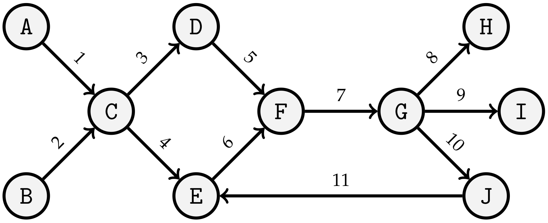
A graph contains nodes which are connected by directed or undirected edges (see Figure 1) [64]. Directed edges create a connection between nodes that points only in one direction [63].
There are several application areas for graphs. Thus they can be used outside of problem solving or mapping networks [64]. In the context of JSP, it can be applied by interpreting tasks as nodes. Predecessor and successor relationships of tasks are represented as directed edges.
Edges can connect two nodes on the one hand, but can also loop back to the same node on the other. Two nodes can also be connected to each other by several edges. This phenomenon is called multiple edges and is contained in a multigraph. If a graph has one of these features, it is no longer called a simple graph [63,65].
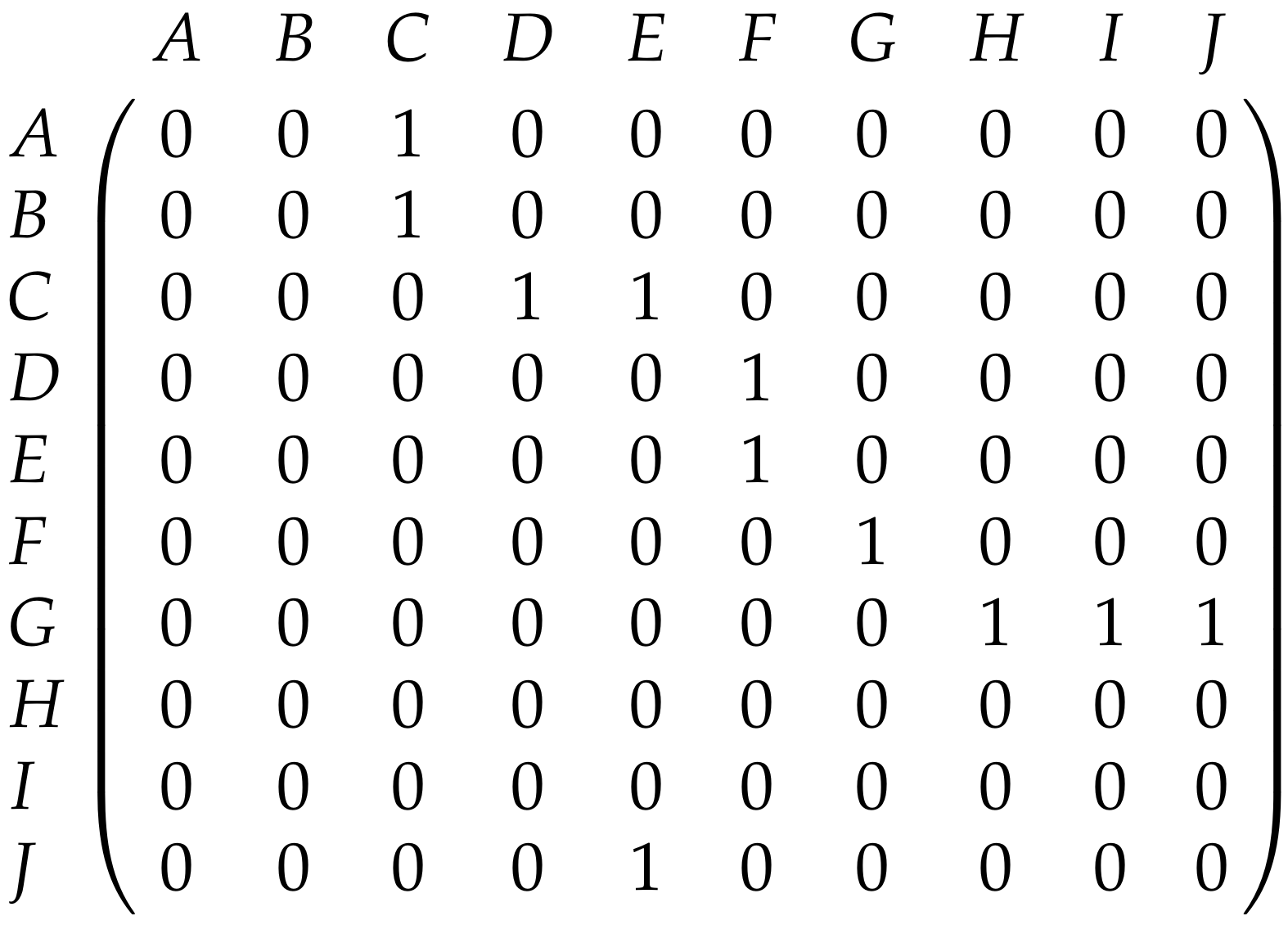
Graphs can be displayed in the form of diagrams or as matrices or lists [66]. However, diagrams can be used to show optically logical relationships in a clearer way. Matrices such as adjacency and incidence matrices can be used for the formal representation of networks. It should be noted that the modified representation does not communicate additional information, but that the representation of a graph as a matrix can be more suitable for further processing of the information [67,68]. The relationship between edges and nodes is called adjacency [69]. Adjacency matrices represent the interconnected nodes in the form of a matrix, where n is the number of nodes (see Figure 2).
3.2. Topology
The relational position of objects to each other is described with topologies. As different as the positional relationships between objects can be, so extensive is the possibility of representation through topological patterns. In product models, the topology reflects the logical processing sequence of tasks.
The basic patterns of this network structure include the lines-, ring-, tree-, star-, and bus-topology, as well as the meshing and the full meshing [70].
In the tree topology, there is only one path between two nodes of the net. All edges—over any other nodes—lead together to a single point. The ring topology reflects a form of connection in which each element has a predecessor and a successor [71]. In the bus topology there is an edge to which all elements of the network are connected. The line topology has a start node and an end node. All elements between these two nodes have exactly one pre- and one successor. If an element exists at which all other elements are connected directly, i.e., directly, it is called a star topology [71]. The tree topology is already a hybrid topology, since it is structured like a star topology, but further nodes connect to those nodes in level 1 [70,72]. If elements of a network are connected several times by further elements, it is a meshing. If there is a direct connection between every single element, it is a full meshing [70]. Other basic patterns can be derived from the topologies mentioned, most of which are based on the tree topology.
3.3. Product Model Topologies
Since models, that are intended to represent the product manufacturing process, can be regarded as a directed graph, basic patterns can also be identified and quantified here (see Table 4):
| Sequence: | A linear sequence of tasks in which a maximum of one predecessor and one successor exists for a node. |
| Splitting: | A completed task is followed up on by multiple other tasks. |
| Parallelism: | The coexistence of several simultaneous tasks, between an expanding and a merging tasks. |
| Merge: | The convergence of several tasks into one subsequent task. |
| Cycle: | One or more tasks may be performed repeatedly. |
| Optionality: | The existence of several, selectable successors of a task. This pattern corresponds to a logical OR operator. |
If the basic patterns just introduced are combined with themselves or with each other, a multitude of new patterns can result (see Table 5):
| Linear: | A linear production process can be represented by stringing together several sequences. |
| Parallel: | A process is split into two linear processes and reunited in a later work step. |
| Multiple Parallel: | The splitting of a process can also take place in more than two sub-sequences, which are merged again at a later point in time. The maximum number of sub-sequences running in parallel depends on the sum of the total number of tasks. |
| Ring: | If each task has exactly one predecessor and one successor, a sequential cycle is created that forms a ring. |
| Tree (splitting): | If the production process is split up after each work step, i.e., the number of tasks increases after each node, this model reflects an initial task with several end products. |
| Tree (merging): | This results in several initial tasks through a continuous combination of the production process, i.e., a reduction in the number of parallel sub-sequences, ultimately in a single final product. |
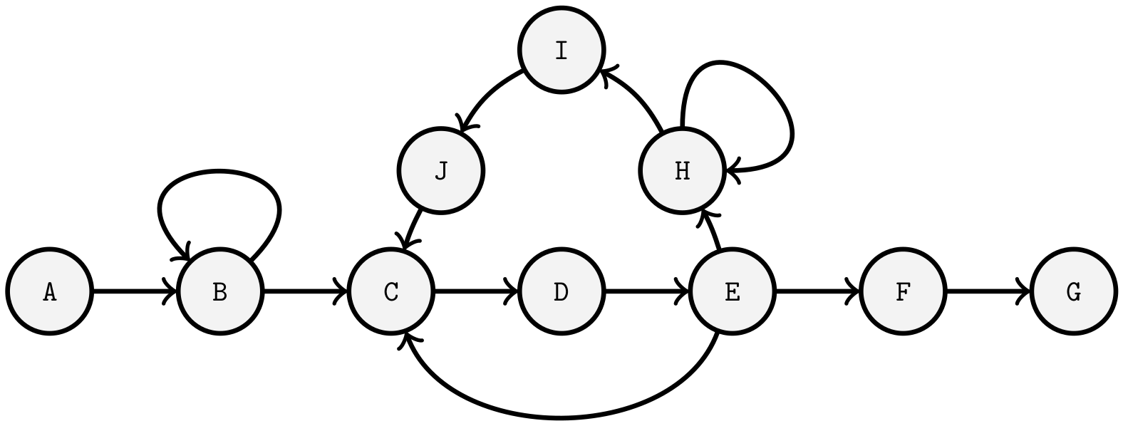
| Cycle: | Recurring tasks can also be present in every pattern presented so far. For example, in a linear sequence of tasks, one or more tasks may have to be performed repeatedly. There may also be additional tasks in a cycle (see Figure 3). |
| Option: | If not every task has to be performed for a product model, then the model contains options. Thus, in a split where at least one subsequent task is optional, parallelism does not have to follow. |
3.4. Complexity of Product Models
Although product models have different topologies, they are serialized in a machine allocation plan as part of a specific scheduling process. This means that there is a binding sequence in which the individual tasks are assigned to a specific time slot on a specific machine.
For products that are created from several tasks running in parallel, first a decision must be made to resolve this parallelism. If, for example, there are two parallel preparatory operations A and B, whose output is then processed by task C to produce a final result, the actual start may begin with either A or B. Depending on resource requirements and other jobs, even those two options can lead to radical changes in the optimization result.
If each work step has two predecessors (that is, seven instead of three work steps in total), the number of valid serializations increases from two to 80 variants (see Table 6). If one more production stage is added, there are already more than 21 million possible combinations, which are caused by only one product of a plan. If, on the other hand, only linear product models are used, there is always only one valid sequence for each product size (seet Table 7). With this extreme simplification, however, they do not cover the real variety of product models.
If only the number of tasks a job consists of is specified for test data, this is not a clear statement of the actual complexity of the problem (see Table 6). With the flow shop scheduling problem, the problem complexity of individual product models is low. If only sequential task sequences can be assumed, there is only one valid serialization variant for each product model (see Table 7).
While the structure of the product models primarily determines the dependencies between individual work steps, the dominance of individual work steps is determined by their processing time. Short work steps are more likely to find a gap in machine schedules. The probability that allocation conflicts will occur on a machine increases with the length of a work step. However, the absolute amount of time is irrelevant. Whether a work step must be regarded as long or short can be determined relatively and only by comparing it with the times of the tasks in other product models.
Minimum and maximum time limits are also specified. Sometimes there are products which have to cool down, dry or mature after one work step. In this case, a certain waiting time must elapse before the next work step can be carried out on the product (minimum waiting time). There are also working steps after which the product may only wait a certain period of time before it can be further processed, e.g., before it unintentionally hardens, contaminates or disintegrates (maximum waiting time).
In the overall view, there are further factors influencing the complexity of the JSP. These include the production plan, which compiles a set of product models and production quantities. On the other hand, it also includes the constraints specified by the production system itself: The number of machines, the capacity of the individual machines, the number of personnel, and the setup times required to prepare a machine for the next work order. However, the definition of these influencing factors is independent of the product models. In practice, however, it is a thoroughly relevant question which modifications to these constraints can most favour a fixed sequence of tasks in execution. These constraints also include the option that a work step can be executed on alternative machine types. The efficiency of the machining process can vary depending on the machine.
All these time specifications and constraints have no influence on the size of the solution space (problem complexity), but on the occurrence of capacity bottlenecks in the concrete task planning in a machine scheduling plan. The solution space is only defined by the number of orders and their number of work steps, product model structure and machine assignment. In order to be able to distinguish basic production types from each other, only the structure of product models is considered at first.
3.5. Metrics of Social Network Analysis
Social Network Analysis (SNA) is applied in divergent domains, both scientific and practical. The method can be applied interdisciplinarily and is useful for the analysis of networks of different types [74].
If actors are connected through relationships, they form a network which can be examined with the help of social network analysis. It is not necessary for the actors of a network to be individuals [75]. Likewise, an analysis of other related objects can also be performed, e.g., tasks within a product model.
Data about actors in a network can be displayed in tabular form, as a series of rows, with the corresponding properties in the columns. They can also be arranged in a matrix, in which the rows represent senders and the columns receivers of information. Thus, each cell always contains information about the relationship between two actors in the network [76].
In the following, metrics of the SNA are described, which are used for the analysis of product models. In this context, product models are regarded as networks. Tasks are represented by nodes. Predecessor/successor relationships between tasks are represented by directed edges.
- Mean degree:
- Also called average degree, is a measure that reflects the interconnection of all nodes of a network by using the arithmetic mean. Here not only directionally connected nodes but all adjacent nodes are considered. The mean weighted degree differs from the mean degree: Its calculation only considers directed, connected nodes and not adjacents [77]:The mean degree is determined by the average of the degrees of the edges k, which is adjacent to the sum N of the nodes. This corresponds to dividing the double of the edge sum L by the sum of nodes N.
- Network diameter:
- Edge density:
- This is the ratio between the number of existing edges and the number of potentially possible directed or undirected edges in the network. The value is between 0 and 1 [80]. The edge density D can be represented by a division of the connections present in the network and the connections possible in the network (see formula 2):Here m denotes the number of edges and N the number of nodes in the network.
- Modularity:
- It describes the simplicity of breaking down a network into individual cliques. A high degree of modularity reflects the highly complex structure of the network [81]:The modularity Q is determined by the decomposition of the network into m cliques, the number of L edges, the number of edges between nodes of the s-th clique and the sum of degrees of nodes of the s-th clique [81].
- Strongly Connected Component:
- In a network, a strongly connected component is a group of nodes in which all nodes are directly or indirectly connected to each other. The length of the paths is not decisive here. In contrast to strongly connected components, the direction is not considered for weakly connected components [82]
- Mean path length:
3.6. Quantitative Systematization through Metrics
Topological features and metrics of the SNA are used to establish further quantitative distinctiveness of product models. This allows product models to be assigned to classes, which enables them to be sorted, compared and grouped. On the other hand, the differences or similarity between two product models can be precisely quantified using the metrics of the SNA.
To illustrate this connection, the SNA metrics are applied to extended basic topological forms and compared in tabular form (see Table 8). With almost the same number of tasks, there are some extreme differences in the SNA results. But even smaller differences are sufficient to recognize and prove topological differences.
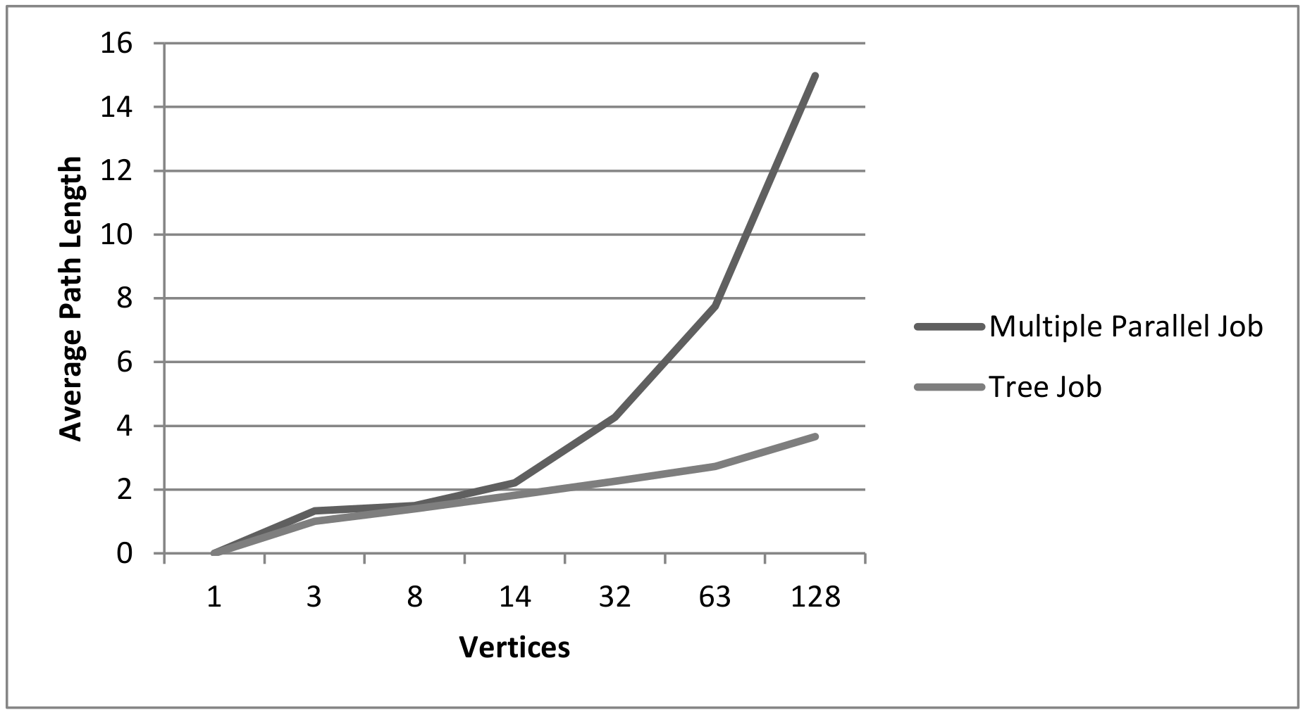
The value of Weakly Connected Components must be 1 in product models. Otherwise it means that there are several separate submodels. Strongly Connected Components, on the other hand, provide feedback on how many different cycles are present in the model. The smaller this value is, the larger are the existing cycles. The maximum number of components corresponds to the existing number of nodes. This implies that there are no built-in feedback loops in the product plans. If the Average Weighted Degree is greater than or equal to 1, this means that parallel or cyclic subprocesses exist. Consistently linear or tree-like structures always have a value below 1, because only a minimal number of edges are used to connect all nodes to each other. A high Network Diameter is an indication for long partial sequences in the model. The value for the Average Path Lenght increases with the Network Diameter. This increase is accelerated by existing cycles.
It should be noted that some special features of structures cannot be derived from the SNA metrics. The metrics do not differ from each other if the models to be compared have the topology of a tree running apart and a tree running together. In order to be able to distinguish these structures from each other, the models must be examined for basic topological forms.
With the exception of the differentiation of tree structures, all topological patterns can be distinguished from each other by the combination of SNA indicators (see Table 9). This is only true for models of the same size. If now two models are compared, an absolute evaluation of structural properties can be made on the basis of the pure metrics (e.g., as for the models in Table 8). Or a relative differentiation can be determined whether, for example, the second model is more similar to another topological basic pattern compared to the first model. In the context of JSP, concrete statements can be made as to which real production scenario these product models can be assigned to (e.g., flow production, recycling, distributed production, variant production, product improvement).
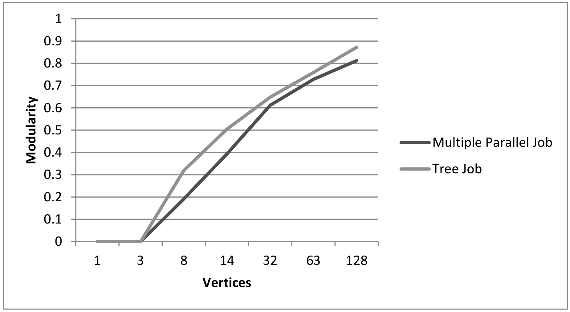
A further problem is that the metric values change with increasing number of nodes but constant topological basic form (see Figure 4, Figure 5 and Figure 6). Inferences to a concrete topology on the basis of these indicators are therefore not trivial. It becomes even more difficult or impossible if a product model combines several basic topological forms and is analysed as a complete model. However, this does not diminish the purpose to prove the difference of two product models.
These metrics can bring benefits if test data is generated in large quantities by random generators. By simultaneously calculating the corresponding metrics, they can be used to form similarity measures for the generated test data. A subsequent cluster analysis makes it possible to recognize patterns in the models’ composition [84]. The composition of the models can be checked for equal distribution by means of the metrics.
4. Obstacles Identified in Method Comparisons Carried Out
The following is a summary of the problems identified in relation to the test data used.
The analysis of these scientific articles, in which, besides pure presentations of optimization methods, comparisons of optimization methods were also accomplished, showed that not only the procedure of comparisons, but also the representation of the results differs strongly from each other.
The form and scope of the presentation and treatment of comparative data used are also not of a homogeneous nature (see Section 2). This on one hand affects on the descriptiveness of the accomplished presentations and comparisons, but on the other hand, the results become less comparable by the different use of models and their description. That a differentiated consideration and description of product models is not only possible but also necessary could be shown on the basis of some characteristic numbers (see Section 3). The following problems can be identified in this entire situation:
- Non-comparability of the search space implicitly predefined by the test data sets (complexity, location of good solutions).
- Incompleteness due to (un)consciously selected test scenarios.
- Non-differentiability due to missing characteristic descriptions for test models.
- Modeling effort.
- Illustrativeness of the scenarios represented by test data is too low and does not allow comparison between simulation and practical scenario.
- Inconsistent representation regarding denominators.
- Missing benchmark due to unknown optimal solution for a test scenario.
Those problem areas will be explained in more detail later on. If comparisons were to be carried out on a ready-made or standardized collection of product models, many of the mentioned disadvantages could be minimized. The lack of standardized test models gives rise to a lack of commitment, systematization and availability.
Non-Comparability
If several benchmarks of methods for JSP are accomplished on the basis of different test data sets, then the results are not directly comparable with each other. The results of the comparisons produced cannot be objectively compared if the characteristics of the models used are not communicated. Advantageous or restrictive influencing of variables for particular optimization methods can already influence the result positively or negatively in the form of number, sequence, or length of the occurrence of tasks in models. If problems of the same size exist, it cannot be determined immediately which of these problems is considered the most severe for an optimization method and so the selection decision has a strongly subjective character [36]. Of course, the size and complexity of models, as well as the type of algorithms compared in the comparisons, has a decisive influence, since, for example, genetic algorithms are more promising in heavier or more complex problem classes than calculating methods.
Incompleteness
Sometimes, it can come to the fact that just such models, which show characteristic values classified as restricting influencing variables for a certain procedure, are not considered within method comparisons. Reasons for a purposeful exclusion can be the missing coverage of certain problem definitions of the optimization procedure, or of the main feature of the optimization method, which is the center of the consideration.
If the non-consideration of certain test cases would be arguable under such conditions, there is nevertheless the difficulty of comparing method comparisons, to find out wether they use only a few identical model sets. This problem can increase with the number of comparisons, because the intersection of all comparisons can decrease. The non-cosideration of particular test data sets my give researchers the impression that the experiment design is incomplete.
Non-Differentiability
If models cannot be differentiated from one another on the basis of objective variables or distinguishing features, it will lead to a lack of differentiability. In this case, the difference cannot be quantified at all. Possible consequences of different models can then no longer be assumed.
Modeling Effort
If no suitable models are available for a research project, if there is unawareness about their existence, or if no selection is possible due to a lack of description, it is necessary to define the required test data sets oneself. The definition of test problems requires a lot of time, which includes the conception as well as the modelling of the test data.
Random number generators are often used to generate test data [36,38,53,55]. Bratley et al. [85] propose in “A Guide to Simulation” a random number generator, which for example Taillard [36] uses to generate random numbers, that are used for the problem instances suggested by himself.
For the useful modelling of test data, which can be used for sequence planning in production planning and control, it must be ensured that the model does not deviate from reality in decisive features [86].
Illustrativeness
Test data are represented abstractly as models of reality, since from the view of the optimization procedures there is no necessity to establish a reference to an existing manufacturing process. In order to exactly depict the actual production of products, considerable information procurement costs and a higher effort in the calculation of results arise which are not usual in scientific practice for economic reasons [86].
However, practice-oriented examples and their visual representation can improve the clarity of result communication, i.e., also of advertising on one’s own behalf. For a test data set, a practical illustration can serve as proof that the test data are capable of mapping realistic scenarios.
Inconsistent Representation
There are differences in the way problems are described. Fisher and Thompson [34] describe problems in the form ‘Jobs’ × ‘Machines’ × ‘Tasks’. Fang et al. [50] use the following representation: ‘Jobs’ × ‘Machines’. Already, the existence of an inconsistency is shown in the description of the problems concerning the mentioned components. A uniform naming regarding the composition of individual jobs regarding the contained tasks could not be observed in the investigated comparisons of optimization methods.
Furthermore, there are differences in the description of the Job-shop problem. Taillard [36] uses a representation form for his problems that deviates from the standard specification for Job-shop problems [87]. By using these two forms of representation, the similarity of two test scenarios cannot always be recognized immediately at first glance, even if two exactly identical product models are used.
Missing Scale
Often, the test data used to compare optimization methods is generated randomly or manually [38].
Here, it is noted that in the examined articles results of preceding research activities were often used as reference point for comparisons. These results are often based on relatively smaller problems of [16,26,27,34] under the aspect of today’s available computing power.
The particular procedures should find optimal or good approximation solutions for the problem cases within the scope of simulations on computers. For smaller and lighter models, which are often used, optimal solutions are usually known, against which the methods can be measured. The situation is different for larger and heavier models, where the optimal solutions may not be available. In these cases, a comparison of the methods can only take place on the basis of solutions which approximate an unknown optimal solution. Thus, these comparisons always remain relative to each other. The time difference in calculation time can be marginal or may be particularly serious when comparing two methods, not allowing a clear statement to be made, considering the solution’s quality. The efficiency of procedures can be assessed more reliably by the presence and comparison of an optimal solution as a benchmark.
5. Discussion and Conclusions
Every JSP researcher is faced with the question of what the test data for his JSP simulation should look like. Objective requirements can be set that are easy to implement and scientifically sound. If the optimization algorithm is at the research’s forefront, there is no reason to derivate from the proven or randomly generated test data for simulation. However, the question arises as to whether the randomness is really sufficiently random for this test context. The context may have to be extremely narrowed down, because even small changes in a set of random data that is supposedly generated in the same way can have extreme effects on the quality of the simulation results. To prevent the test data from being compared with each other, when it should be the optimization methods, standardized test data are advantageous. However, these must be generated transparently and in two ways. On one hand, the characteristics of the test data must be known. It must be comprehensible why which design decisions and compilations were made for which application context. In addition, it must be clear how the selection process for these test data took place. This is because the selection must not favour any actor in order to not distort scientific and economic competition for efficient procedures.
There is no ideal solution for the form in which the product models should be designed. A seemingly good solution has no value if it is not used by the JSP research community. On the other hand, even minimal or poor solutions offer great added value, because the scientific connectivity of research results is enhanced by standards for test data. The evaluation of a solution for the editing of test data can therefore only be carried out by the JSP reseach community on the basis of consensus. This contribution is intended to sensitize and inspire.
It is not only the Operations Research (OR) researchers who are interested in JSP test data sets. Software developers need test data to verify their implementation and to check runtime behavior. Software vendors need comprehensible test scenarios for product presentation. Consultants for the introduction of JSP software need vendor-independent test data that corresponds to the typical orders of the company to be advised. Illustrative test data is required for JSP and OR education and training. Developers of production systems need test data to simulate the effects of alternative investment scenarios (number and type of machines). Lastly, even an operational dispatcher can need test data to reach the limits of the feasibility of concrete daily schedules. All these actors create their own test data and each is at risk of misconfiguration. There is no sustainable reason not to develop common test data strategy and management.
The general discussion about Open Access for test data is ongoing [9,88,89,90] and also concerns JSP research. The mere availability of individual product models or entire test plans is only one step in this direction. The next step is a standardized, systematic representation, combinability, and selection of those test data. Another step is the agreement on certain test data, which are to be used a as standard for certain test series, problems, and research goals. This is the only way to give the users of these test data a binding basis on which to orient themselves and make the right choice for their respective research questions. Building on this, procedure models can then be developed for standardized testing of the performance of JSP methods and their documentation.
Author Contributions
Conceptualization, N.G., E.W. and A.T.; methodology, E.W. and A.T.; formal analysis, E.W. and A.T.; investigation, A.T.; writing—original draft preparation, E.W. and A.T.; writing—review and editing, E.W.; visualization, A.T.; supervision, N.G.; funding acquisition, N.G.
Funding
This research was funded by the Germen Research Foundation grant number GR 1846/17-1.
Conflicts of Interest
The authors declare no conflict of interest. The funders had no role in the design of the study; in the collection, analyses, or interpretation of data; in the writing of the manuscript, or in the decision to publish the results.
Abbreviations
The following abbreviations are used in this manuscript:
| JSP | Job-Shop Scheduling Problem |
| SNA | Social Network Analysis |
References
- Cheng, R.; Gen, M.; Tsujimura, Y. A Tutorial Survey of Job-Shop Scheduling Problems Using Genetic Algorithms—Representation. Comput. Ind. Eng. 1996, 30, 983–997. [Google Scholar] [CrossRef]
- Dell’Amico, M.; Trubian, M. Applying Tabu Search to the Job-Shop Scheduling Problem. Ann. Oper. Res. 1993, 41, 231–252. [Google Scholar] [CrossRef]
- Fischäder, H.; Göhler, R.; Schneider, H.M. Maschinenbelegungsplanung in entkoppelten Produktionssystemen. productivITy 2017, 22, 1–20. [Google Scholar]
- Scharbrodt, M. Produktionsplanung in der Prozessindustrie: Modelle, Effziente Algorithmen und Umsetzung. Ph.D. Thesis, Technical University of Munich, Munich, Germany, October 2000. [Google Scholar]
- Carlier, J.; Pinson, E. An Algorithm for Solving the Job-Shop Problem. Manag. Sci. 1989, 35, 164–176. [Google Scholar] [CrossRef]
- Applegate, D.; Cook, W. A Computational Study of the Job-Shop Scheduling Problem. ORSA J. Comput. 1991, 3, 149–156. [Google Scholar] [CrossRef]
- Nakano, R.; Yamada, T. Conventional Genetic Algorithm for Job Shop Problems. In Proceedings of the 4th International Conference on Genetic Algorithms, San Diego, CA, USA, 13–16 July 1991; Volume 91, pp. 474–479. [Google Scholar]
- Nowicki, E.; Smutnicki, C. An Advanced Tabu Search Algorithm for the Job Shop Problem. J. Sched. 2005, 8, 145–159. [Google Scholar] [CrossRef]
- Van den Eynden, V.; Corti, L.; Wollard, M.; Bishop, L.; Horton, L. Managing and Sharing Data: A Best Practice Guide for Researchers, 3rd ed.; UK Data Archive University of Essex: Colchester, UK, 2011; OCLC: 727970452. [Google Scholar]
- Vahrenkamp, R. Produktionsmanagement, 6th ed.; Oldenbourg Verlag: Wien, Austria, 2008. [Google Scholar]
- Fischäder, H.; Göhler, R.; Schneider, H.M. Maschinenbelegungsplanung in Mehrstufigen Produktionssystemen. Ph.D. Thesis, Technische Universitat Ilmenau, Ilmenau, Germany, 2017. Volume 22. pp. 29–32. [Google Scholar]
- Henning, A. Praktische Job-Shop Scheduling-Probleme. Ph.D. Thesis, Friedrich Schiller University, Jena, Germany, August 2002. [Google Scholar]
- Käschel, J.; Teich, T. Reihenfolgeplanung in Produktionsnetzwerken. In IT-gestützte Betriebswirtschaftliche Entscheidungsprozesse; Jahnke, B., Wall, F., Eds.; Gabler Verlag: Wiesbaden, Germany, 2001; pp. 239–259. [Google Scholar]
- Pinedo, M. Scheduling: Theory, Algorithms, and Systems, 5th ed.; Springer: Berlin, Germany, 2016. [Google Scholar]
- Gronau, N.; Weber, E. Reihenfolgeplanung Im Zeitalter von Industrie 4.0. productivITy 2018, 23, 23–26. [Google Scholar] [CrossRef]
- Muth, J.F.; Thompson, G.L. Industrial Scheduling; Prentice Hall: Englewood Cliffs, NJ, USA, 1963. [Google Scholar]
- Baker, K.R. Introduction to Sequencing and Scheduling; Wiley: Hoboken, NJ, USA, 1974; Open Library ID: OL5047415M. [Google Scholar]
- Lenstra, J.K.; Rinnooy Kan, A.H.G.; Brucker, P. Complexity of Machine Scheduling Problems. In Studies in Integer Programming; Hammer, P.L., Johnson, E.L., Korte, B.H., Nemhauser, G.L., Eds.; Elsevier: Amsterdam, The Netherlands, 1977; Volume 1, pp. 343–362, Annals of Discrete Mathematics. [Google Scholar]
- Rinnooy Kan, A.H.G. Machine Scheduling Problems—Classification, Complexity and Computations; Springer US: New York, NY, USA, 1976; OCLC: 863792546. [Google Scholar]
- French, S. Sequencing and Scheduling: An Introduction to the Mathematics of the Job-Shop; Ellis Horwood Series in Mathematics and Its Applications; Wiley: Hoboken, NJ, USA, 1982. [Google Scholar]
- Conway, R.W.; Maxwell, W.L.; Miller, L.W. Theory of Scheduling; Courier Corporation: Washington, DC, USA, 1967. [Google Scholar]
- Dorndorf, U.; Pesch, E. Evolution Based Learning in a Job Shop Scheduling Environment. Comput. Oper. Res. 1995, 22, 25–40. [Google Scholar] [CrossRef]
- Jain, A.S.; Meeran, S. A State-of-the-Art Review of Job-Shop Scheduling Techniques; Technical Report; University of Dundee: Scotland, UK, 1998. [Google Scholar]
- Manne, A.S. On the Job-Shop Scheduling Problem. Oper. Res. 1960, 8, 219–223. [Google Scholar] [CrossRef]
- Barker, J.R.; McMahon, G.B. Scheduling the General Job-Shop. Manag. Sci. 1985, 31, 594–598. [Google Scholar] [CrossRef]
- Lawrence, S.R. Resource Constrained Project Scheduling: An Experimental Investigation of Heuristic Scheduling Techniques (Supplement); Graduate School of Industrial Administration, Carnegie-Mellon University: Pittsburgh, PA, USA, 1984. [Google Scholar]
- Adams, J.; Balas, E.; Zawack, D. The Shifting Bottleneck Procedure for Job Shop Scheduling. Manag. Sci. 1988, 34, 391–401. [Google Scholar] [CrossRef]
- Beasley, J.E. OR-Library: Distributing Test Problems by Electronic Mail. J. Oper. Res. Soc. 1990, 41, 1069–1072. [Google Scholar] [CrossRef]
- Beasley, J.E. OR-LIBRARY. 1990. Available online: http://people.brunel.ac.uk/ mastjjb/jeb/info.html (accessed on 1 December 2018).
- Van Hoorn, J. Job Shop Instances and Solutions. 2015. Available online: http://jobshop.jjvh.nl/ (accessed on 1 December 2018).
- Shylo, O. Job Shop Scheduling. 2018. Available online: http://optimizizer.com/jobshop.php (accessed on 1 December 2018).
- Tamura, Y. JSPLIB: Benchmark Instances for Job-Shop Scheduling Problem. 2018. Available online: https://github.com/tamy0612/JSPLIB (accessed on 1 December 2018).
- Staples, M.; Niazi, M. Experiences Using Systematic Review Guidelines. J. Syst. Softw. 2007, 80, 1425–1437. [Google Scholar] [CrossRef]
- Fisher, H.; Thompson, G.L. Probabilistic Learning Combinations of Local Job-Shop Scheduling Rules. In Industrial Scheduling; Muth, J.F., Thompson, G.L., Eds.; Prentice Hall: Upper Saddle River, NJ, USA, 1963; pp. 225–251. [Google Scholar]
- Giffler, B.; Thompson, G.L.; Van Ness, V. Numerical Experience with the Linear and Monte Carlo Algorithms for Solving Production Scheduling Problems. In Industrial Scheduling; Muth, J.F., Thompson, G.L., Eds.; Prentice Hall: Upper Saddle River, NJ, USA, 1963; pp. 21–38. [Google Scholar]
- Taillard, E. Benchmarks for Basic Scheduling Problems. Eur. J. Oper. Res. 1993, 64, 278–285. [Google Scholar] [CrossRef]
- Bierwirth, C. A Generalized Permutation Approach to Job Shop Scheduling with Genetic Algorithms. Oper.-Res.-Spektrum 1995, 17, 87–92. [Google Scholar] [CrossRef]
- Nowicki, E.; Smutnicki, C. A Fast Taboo Search Algorithm for the Job Shop Problem. Manag. Sci. 1996, 42, 797–813. [Google Scholar] [CrossRef]
- Vázquez, M.; Whitley, L.D. A Comparison of Genetic Algorithms for the Dynamic Job Shop Scheduling Problem. In Proceedings of the 2nd Annual Conference on Genetic and Evolutionary Computation, Las Vegas, NV, USA, 10–12 July 2000; Morgan Kaufmann Publishers Inc.: San Mateo, CA, USA, 2000; pp. 1011–1018. [Google Scholar]
- Bratley, P.; Florian, M.; Robillard, P. On Sequencing with Earliest Starts and Due Dates with Application to Computing Bounds for the (n/m/G/Fmax) Problem. Naval Res. Logist. Quart. 1973, 20, 57–67. [Google Scholar] [CrossRef]
- Brucker, P.; Jurisch, B.; Sievers, B. A Branch and Bound Algorithm for the Job-Shop Scheduling Problem. Discrete Appl. Math. 1994, 49, 107–127. [Google Scholar] [CrossRef]
- McMahon, G.; Florian, M. On Scheduling with Ready Times and Due Dates to Minimize Maximum Lateness. Oper. Res. 1975, 23, 475–482. [Google Scholar] [CrossRef]
- Lenstra, J.K. Sequencing by Enumerative Methods; Number 69 in Mathematical Centre Tract; Mathematisch Centrum: Amsterdam, The Netherlands, 1976; A Revision of Author’s Thesis, Mathematisch Centrum, Amsterdam. [Google Scholar]
- Carlier, J. Ordonnancements à Contraintes Disjonctives. Thèse de 3ème cycles. Ph.D. Thesis, Paris 6 University, Paris, France, November 1978. [Google Scholar]
- Kim, Y.D. A Comparison of Dispatching Rules for Job Shops with Multiple Identical Jobs and Alternative Routeings. Int. J. Prod. Res. 1990, 28, 953–962. [Google Scholar] [CrossRef]
- Nasr, N.; Elsayed, E.A. Job Shop Scheduling with Alternative Machines. Int. J. Prod. Res. 1990, 28, 1595–1609. [Google Scholar] [CrossRef]
- Storer, R.H.; Wu, S.D.; Vaccari, R. New Search Spaces for Sequencing Problems with Application to Job Shop Scheduling. Manag. Sci. 1992, 38, 1495–1509. [Google Scholar] [CrossRef]
- Yamada, T.; Nakano, R. A Genetic Algorithm Applicable to Large-Scale Job-Shop Problems. Parallel Proble. Solving Nat. 1992, 2, 283–292. [Google Scholar]
- Van Laarhoven, P.J.M.; Aarts, E.H.L.; Lenstra, J.K. Job Shop Scheduling by Simulated Annealing. Oper. Res. 1992, 40, 113–125. [Google Scholar] [CrossRef]
- Fang, H.L.; Ross, P.; Corne, D. A Promising Genetic Algorithm Approach to Job-Shop Scheduling, Re-Scheduling and Open-Shop Scheduling Problems. Available online: http://homepages.inf.ed.ac.uk/rbf/MY_DAI_OLD_FTP/rp623.pdf (accessed on 18 February 2019).
- Aarts, E.H.L.; Van Laarhoven, P.J.M.; Lenstra, J.K.; Ulder, N.L.J. A Computational Study of Local Search Algorithms for Job Shop Scheduling. ORSA J. Comput. 1994, 6, 118. [Google Scholar] [CrossRef]
- Aarts, E.H.L.; Van Laarhoven, P.J.M.; Ulder, N.L.J. Local-Search-Based Algorithms for Job Shop Scheduling; Working Paper; Eindhoven University of Technology: Eindhoven, The Netherlands, 1991. [Google Scholar]
- Demirkol, E.; Mehta, S.; Uzsoy, R. Benchmarks for Shop Scheduling Problems. Eur. J. Oper. Res. 1998, 109, 137–141. [Google Scholar] [CrossRef]
- Morton, T.E.; Pentico, D. Heuristic Scheduling Systems: With Applications to Production Systems and Project Management, 1st ed.; John Wiley and Sons: New York, NY, USA, 1993. [Google Scholar]
- Vázquez, M.; Whitley, L.D. A Comparison of Genetic Algorithms for the Static Job Shop Scheduling Problem; Parallel Problem Solving from Nature PPSN VI; Lecture Notes in Computer Science; Springer: Berlin, Germany, 2000; pp. 303–312. [Google Scholar]
- Watson, J.P.; Barbulescu, L.; Howe, A.E.; Whitley, L.D. Algorithm Performance and Problem Structure for Flow-Shop Scheduling. In Proceedings of the AAAI-99 Proceedings, American Association for Artificial Intelligence, Orlando, FL, USA, 18–22 July 1999; pp. 688–695. [Google Scholar]
- Aiex, R.M.; Binato, S.; Resende, M.G.C. Parallel GRASP with Path-Relinking for Job Shop Scheduling. Parallel Comput. 2003, 29, 393–430. [Google Scholar] [CrossRef]
- Chong, C.S.; Sivakumar, A.I.; Low, M.Y.H.; Gay, K.L. A Bee Colony Optimization Algorithm to Job Shop Scheduling. In Proceedings of the 38th Conference on Winter Simulation. Winter Simulation Conference, Monterey, CA, USA, 3–6 December 2006; pp. 1954–1961. [Google Scholar]
- Özgüven, C.; Özbakır, L.; Yavuz, Y. Mathematical Models for Job-Shop Scheduling Problems with Routing and Process Plan Flexibility. Appl. Math. Modell. 2010, 34, 1539–1548. [Google Scholar] [CrossRef]
- Fattahi, P.; Mehrabad, M.S.; Jolai, F. Mathematical Modeling and Heuristic Approaches to Flexible Job Shop Scheduling Problems. J. Intell. Manuf. 2007, 18, 331–342. [Google Scholar] [CrossRef]
- Mousavi, S.; Zandieh, M.; Amiri, M. Comparisons of Bi-Objective Genetic Algorithms for Hybrid Flowshop Scheduling with Sequence-Dependent Setup Times. Int. J. Prod. Res. 2012, 50, 2570–2591. [Google Scholar] [CrossRef]
- Fisher, M.L. A Dual Algorithm for the One-Machine Scheduling Problem. Math. Programm. 1976, 11, 229–251. [Google Scholar] [CrossRef]
- Brandes, U. Graphentheorie. In Handbuch Netzwerkforschung; Stegbauer, C., Häußling, R., Eds.; VS Verlag für Sozialwissenschaften: Wiesbaden, Germany, 2010; pp. 345–353. [Google Scholar]
- Stegbauer, C.; Häussling, R. (Eds.) Netzwerkforschung. Handbuch Netzwerkforschung, 1st ed.; VS Verlag für Sozialwissenschaften: Wiesbaden, Germany, 2010; Volume 4. [Google Scholar]
- Bondy, J.A. Basic Graph Theory: Paths and Circuits. In Handbook of Combinatorics; Graham, R.L., Grötschel, M., Lovász, L., Eds.; MIT Press: Cambridge, MA, USA, 1995; Volume 1, pp. 3–110. [Google Scholar]
- Turau, V. Algorithmische Graphentheorie; Oldenbourg: Wien, Austria, 2009; OCLC: 467891833; 3, überarb, aufl. [Google Scholar]
- Lerner, J. Beziehungsmatrix. In Handbuch Netzwerkforschung; VS Verlag für Sozialwissenschaften: Wiesbaden, Germany, 2010; pp. 355–364. [Google Scholar]
- Kaderali, F.; Poguntke, W. Graphen Algorithmen Netze: Grundlagen und Anwendungen in der Nachrichtentechnik; Vieweg: Braunschweig, Germany, 1995. [Google Scholar]
- Hohberger, S.; Damlachi, H. Praxishandbuch Sanierung im Mittelstand; Springer Fachmedien: Wiesbaden, Germany, 2014. [Google Scholar]
- Pandya, K. Network Structure or Topology. Int. J. Adv. Res. Comput. Sci. Manag. Stud. 2013, 1, 22–27. [Google Scholar]
- Abts, D.; Mülder, W. Grundkurs Wirtschaftsinformatik: Eine Kompakte und Praxisorientierte Einführung, 9th ed.; Springer Vieweg: Berlin, Germany, 2002. [Google Scholar]
- Ernst, H.; Schmidt, J.; Beneken, G.H. Grundkurs Informatik: Grundlagen und Konzepte für die Erfolgreiche IT-Praxis; Eine Umfassende, Praxisorientierte Einführung, 5th ed.; Lehrbuch, Springer Vieweg: Berlin, Germany, 2015; OCLC: 907482533. [Google Scholar]
- Tanenbaum, A.S.; Wetherall, D.J. Computer Networks, 5th ed.; Pearson Prentice Hall: Upper Saddle River, NJ, USA, 2011; OCLC: ocn660087726. [Google Scholar]
- Baumöl, U.; Ickler, H. Soziale Netzwerkanalyse. In Enzyklopädie der Wirtschaftsinformatik, 10th ed.; Gronau, N., Becker, J., Kliewer, N., Leimeister, J.M., Overhage, S., Eds.; GITO: Berlin, Germany, 2018. [Google Scholar]
- Stegbauer, C. Soziale Netzwerkanalyse. In Handbuch Medienpädagogik; VS Verlag für Sozialwissenschaften: Wiesbaden, Germany, 2008; pp. 166–172. [Google Scholar]
- Rürup, M.; Röbken, H.; Emmerich, M.; Dunkake, I. Netzwerke im Bildungswesen; Springer Fachmedien Wiesbaden: Wiesbaden, Germany, 2015. [Google Scholar]
- Ayyappan, G.; Nalini, D.C.; Kumaravel, D.A. A Study on SNA: Measure Average Degree and Average Weighted Degree of Knowledge Diffusion in GEPHI. Indian J. Comput. Sci. Eng. (IJCSE) 2016, 7, 230–237. [Google Scholar]
- Bojic, I.; Lipic, T.; Podobnik, V. Bio-Inspired Clustering and Data Diffusion in Machine Social Networks. In Computational Social Networks; Abraham, A., Ed.; Springer: Berlin, Germany, 2012; pp. 51–79. [Google Scholar]
- Barabási, A.L.; Pósfai, M. Network Science; Cambridge University Press: Cambridge, UK, 2016. [Google Scholar]
- Ghali, N.; Panda, M.; Hassanien, A.E.; Abraham, A.; Snasel, V. Social Networks Analysis: Tools, Measures and Visualization. In Computational Social Networks: Mining and Visualization; Abraham, A., Ed.; Springer: Berlin, Germany, 2012; pp. 3–23. [Google Scholar]
- Catanese, S.; De Meo, P.; Ferrara, E.; Fiumara, G.; Provetti, A. Extraction and Analysis of Facebook Friendship Relations. In Computational Social Networks: Mining and Visualization; Abraham, A., Ed.; Springer: Berlin, Germany, 2012; pp. 291–324. [Google Scholar]
- Easley, D.; Kleinberg, J. Networks, Crowds, and Markets: Reasoning about a Highly Connected World; Cambridge University Press: Cambridge, UK, 2010. [Google Scholar]
- Wu, H.; Gu, X.; Zhao, Y. The Empirical Study of a Sna-Based Approach for Identifying KSC of Enterprise. Chem. Eng. Trans. 2015, 2, 1291–1296. [Google Scholar]
- Wiedenbeck, M.; Züll, C. Clusteranalyse. In Handbuch der Sozialwissenschaftlichen Datenanalyse, 1st ed.; Wolf, C., Best, H., Eds.; VS Verlag für Sozialwissenschaften: Wiesbaden, Germany, 2010; pp. 525–552. [Google Scholar]
- Bratley, P.; Fox, B.L.; Schrage, L.E. A Guide to Simulation, 2nd ed.; Springer: Berlin, Germany, 1987. [Google Scholar]
- Georgi, G. Job Shop Scheduling in der Produktion; Wirtschaftswissenschaftliche Beiträge; Physica-Verlag: Heidelberg, Germany, 1995; Volume 111. [Google Scholar]
- Van Hoorn, J. Jobshop Explanations. 2015. Available online: http://jobshop.jjvh.nl/explanation.php (accessed on 1 December 2018).
- Organisation for Economic Co-Operation and Development. OECD Principles and Guidelines for Access to Research Data from Public Funding; OECD Publishing: Paris, France, 2007. [Google Scholar]
- Nicol, A.; Caruso, J.; Archambault, E. Open Data Access Policies and Strategies in the European Research Area and Beyond; Technical Report RTD-B6-PP-2011-2; European Commission DG Research & Innovation: Brussels, Belgium, 2013. [Google Scholar]
- Mishra, S. (Ed.) Concepts of Openness and Open Access; United Nations Educational, Scientific and Cultural Organization: Paris, France, 2015. [Google Scholar]
| 1. | It was refered to the OR-Library. Primary sources were not mentioned. |
Figure 1.
Example of a directed graph.

Figure 2.
Adjacency matrix of the graph from Figure 1.
Figure 2.
Adjacency matrix of the graph from Figure 1.

Figure 3.
Topology with multiple cycles.

Figure 4.
Comparison of mean path length with increasing model size.

Figure 5.
Comparison of modularity with increasing model size.

Figure 6.
Comparison of the mean degree with increasing model size.


Table 1.
Summary of the text analysis of Brucker et al. [41].
Table 1.
Summary of the text analysis of Brucker et al. [41].
| Brucker et al. [41]—“A Branch and Bound Algorithm for the Job-Shop Scheduling Problem” [41] |
|---|
| Brucker et al. [41] describe in their work a developed algorithm to solve the known problem of the size from the work of Muth and Thompson [16] on a workstation in 16 minutes. It is stated that the algorithm—if used as a heuristic—is superior to the results of Adams et al. [27] in optimizing sequence problems up to a size of . Brucker et al. [41] present the details of their optimization method in detail and outline the basic idea of the Branch-and Bound method. The calculated results of 45 problems of different sizes are presented. The problems include between five and 15 machines and between 10 and 30 jobs. Three of these problems come from “Industrial Scheduling” by Muth and Thompson [16] and 42 were created by Adams et al. [27]. |
Table 2.
Summary of the text analysis of Nowicki and Smutnicki [38].
Table 2.
Summary of the text analysis of Nowicki and Smutnicki [38].
| Nowicki and Smutnicki [38]—“A Fast Taboo Search Algorithm for the Job Shop Problem” [38] |
|---|
| Nowicki and Smutnicki [38] present in “A Fast Taboo Search Algorithm for the Job Shop Problem” a taboo search algorithm, which pursues the goal to find the minimum lead time in workshop production. It was tested on a PC with up to 10 000 operations and solved a 10 × 10 serious problem in less than 30 s [38]. Therefore the algorithm TSAB was implemented in Pascal and C on an AT 386DX PC. It was then tested against the following problems. Three problems of Fisher and Thompson [34], abbreviated: FS1, FS2, FS3, with the sizes 6 × 6, 10 × 10 and 5 × 20 [34] as well as two problems with the size 10 × 10 of Adams et al. [27]. Furthermore, tests were performed on 40 problems with eight different sizes (10 × 10, 10 × 15, 10 × 20, 10 × 30, 5 × 10, 5 × 15, 5 × 20, 50 × 15) by Lawrence [26]. [26] was performed. Also 80 problems of Taillard [36] with eight different sizes (15 × 15, 15 × 20, 20 × 20, 15 × 30, 20 × 30, 15 × 50, 20 × 50, 20 × 100) were considered [38]. |
Table 3.
Test models used for the investigation of Job Shop Scheduling Problem (JSP)-optimization algorithms.
Table 3.
Test models used for the investigation of Job Shop Scheduling Problem (JSP)-optimization algorithms.
| Authors | Year | Algorithms | Plans/Problems | Machines | Jobs | Models Used | Sources Refered by Authors |
|---|---|---|---|---|---|---|---|
| Fisher and Thompson [34] | 1963 | 3 | 3 | 5–10 | 6–20 | ||
| Bratley et al. [40] | 1973 | 1 | N/A | 1 | 20–50 | randomly generated | |
| 2 | 80 | N/A | N/A | Conway et al. [21] | Conway et al. [21] | ||
| 2 | 3 | 5–10 | N/A | Fisher and Thompson [34] | Muth and Thompson [16] | ||
| McMahon and Florian [42] | 1975 | 1 | N/A | N/A | 20–50 | Bratley et al. [40] | Bratley et al. [40] |
| 2 | 3 | 5–10 | N/A | Fisher and Thompson [34] | Muth and Thompson [16] | ||
| Barker and McMahon [25] | 1985 | 1 | incomplete information | incomplete information | N/A | N/A | N/A |
| 1985 | 1 | 3 | 5–10 | N/A | Fisher and Thompson [34] | Muth and Thompson [16] | |
| Adams et al. [27] | 1988 | 2–3 | 9 + 21 | 10–15 | 10–50 | self-developed | |
| 2–3 | 1 | 5 | 4 | Lenstra [43] | Lenstra [43] | ||
| 2–3 | 3 | 5–10 | 6–20 | Fisher and Thompson [34] | Muth and Thompson [16] | ||
| 2–3 | 6 | 10 | 15–30 | Lawrence [26] | Lawrence [26] | ||
| Carlier and Pinson [5] | 1989 | 1 | approx. 150 | N/A | N/A | Fisher and Thompson [34], Carlier [44], randomly generated | Muth and Thompson [16], Carlier [44] |
| Kim [45] | 1990 | 29 | 150 | 10–25 | |||
| Nasr and Elsayed [46] | 1990 | 2 | 15 | N/A | N/A | N/A | N/A |
| Applegate and Cook [6] | 1991 | 1 | 3 | N/A | N/A | Fisher and Thompson [34] | Muth and Thompson [16] |
| 1 | 40 | N/A | N/A | Adams et al. [27] | Adams et al. [27] | ||
| 1 | 5 | N/A | N/A | Lawrence [26] | Lawrence [26] | ||
| 1 | 5 | N/A | N/A | Applegate and Cook [6], self-developed | |||
| Nakano and Yamada [7] | 1991 | 1(3) | 3 | 5–10 | 6–20 | Fisher and Thompson [34] | Muth and Thompson [16] |
| Storer et al. [47] | 1992 | 2(9) | 2 | 5–10 | 10–20 | Fisher and Thompson [34] | Muth and Thompson [16] |
| 2(9) | 20 | 10–15 | 20–50 | Storer et al. [47], self-developed | |||
| Yamada and Nakano [48] | 1992 | N/A (≥7) | 3 | 5–10 | 6–20 | Fisher and Thompson [34] | Muth and Thompson [16] |
| N/A (≥7) | 4 | 20 | 20 | self-developed | |||
| van Laarhoven et al. [49] | 1992 | 4 | 3 | 5–10 | 6–20 | Fisher and Thompson [34] | Fisher and Thompson [34] |
| 4 | 40 | 5–15 | 10–30 | Lawrence [26] | Lawrence [26] | ||
| Fang et al. [50] | 1993 | 1(3) | 2 | 5–10 | 10–20 | Fisher and Thompson [34] | Muth and Thompson [16] JSSP |
| 1(3) | 6 | 4–20 | 4–20 | [28] | [28] | ||
| Taillard [36] | 1993 | 1 | 80 | 15–20 | 15–100 | randomly generated | |
| 1 | 120 | 5–20 | 20–500 | randomly generated | |||
| 1 | 60 | 4–20 | 4–20 | randomly generated | |||
| Brucker et al. [41] | 1994 | 1 | 3 | 5–10 | 6–20 | Fisher and Thompson [34] | Muth and Thompson [16] |
| 1 | 42 | 5–15 | 10–30 | Adams et al. [27] | Adams et al. [27] | ||
| Aarts et al. [51] | 1994 | 7 | 3 | 5–10 | 6–20 | Fisher and Thompson [34] | Fisher and Thompson [34] |
| 7 | 40 | 5–15 | 10–30 | Lawrence [26] | Lawrence [26] | ||
| 2 | 3 | 15 | 20 | Adams et al. [27] | Applegate and Cook [6], Adams et al. [27] | ||
| 2 | 7 | 10–15 | 15–20 | Lawrence [26] | Applegate and Cook [6], Adams et al. [27] | ||
| Bierwirth [37] | 1995 | 9 | 2 | 5–10 | 10–20 | Fisher and Thompson [34] | Applegate and Cook [6] |
| 6 | 10 | 10–15 | 15–20 | Lawrence [26] | Applegate and Cook [6] | ||
| Dorndorf and Pesch [22] | 1995 | 6 | 3 | 5–10 | 6–20 | Fisher and Thompson [34] | Fisher and Thompson [34] |
| 6 | 105 (x5) | N/A | N/A | randomly generated | |||
| 6 | 35 | 5–15 | 10–20 | Lawrence [26] | Adams et al. [27], van Laarhoven et al. [49], Aarts et al. [52] | ||
| Nowicki and Smutnicki [38] | 1996 | 7 | 3 | 5–10 | 6–20 | Fisher and Thompson [34] | Fisher and Thompson [34], van Laarhoven et al. [49] |
| 7 | 2 | 10 | 10 | Adams et al. [27] | Adams et al. [27] | ||
| 7 | 40 | 5–15 | 10–30 | Lawrence [26] | Lawrence [26], van Laarhoven et al. [49] | ||
| 7 | 80 | 15–20 | 15–100 | Taillard [36] | Taillard [36] | ||
| 7 | 40 | 5–10 | 500–1000 | randomly generated | |||
| Demirkol et al. [53] | 1998 | N/A (≥3) | 600 | 15–20 | 20–50 | randomly generated | |
| Vázquez and Whitley [39] | 2000 | 6 | 12 | 3–8 | 10–50 | N/A | Morton and Pentico [54] |
| Vázquez and Whitley [55] | 2000 | 5 | 3 | 5–10 | 6–20 | Fisher and Thompson [34] | OR-Library1 |
| 5 | 4 | 20 | 20 | Yamada and Nakano [48] | OR-Library | ||
| 5 | 4 | 10–15 | 10–20 | Lawrence [26] | OR-Library | ||
| 5 | 10 | 20 | 30 | Taillard [36] | OR-Library | ||
| 4 | 16 | 10–20 | 10–20 | self-developed | [56] | ||
| Aiex et al. [57] | 2003 | 2 | 5 | 10–20 | 10–15 | Adams et al. [27] | [28] |
| 2 | 8 | 4–9 | 7–14 | Carlier [44] | [28] | ||
| 2 | 3 | 5–10 | 6–20 | Fisher and Thompson [34] | [28] | ||
| 2 | 10 | 10 | 10 | Applegate and Cook [6] | [28] | ||
| 2 | 40 | 5–15 | 10–30 | Lawrence [26] | [28] | ||
| Nowicki and Smutnicki [8] | 2005 | 4 | 3 | N/A | N/A | Fisher and Thompson [34] | Fisher and Thompson [34] |
| 4 | 40 | N/A | N/A | Lawrence [26] | Lawrence [26] | ||
| 4 | 5 | N/A | N/A | Adams et al. [27] | Adams et al. [27] | ||
| 4 | 10 | N/A | N/A | Applegate and Cook [6] | Applegate and Cook [6] | ||
| 4 | 4 | 20 | 20 | Yamada and Nakano [48] | Yamada and Nakano [48] | ||
| 4 | 20 | 10–15 | 20–50 | Storer et al. [47] | Storer et al. [47] | ||
| 4 | 80 | 15–20 | 15–100 | Taillard [36] | Taillard [36] | ||
| 4 | 80 | N/A | N/A | Demirkol et al. [53] | Demirkol et al. [53] | ||
| Chong et al. [58] | 2006 | 3 | 82 in total | 5–20 | 6–50 | ||
| 3 | 3 | N/A | N/A | Fisher and Thompson [34] | Fisher and Thompson [34] | ||
| 3 | 40 | N/A | N/A | Lawrence [26] | Lawrence [26] | ||
| 3 | 20 | N/A | N/A | Storer et al. [47] | Storer et al. [47] | ||
| 3 | 10 | N/A | N/A | Applegate and Cook [6] | Applegate and Cook [6] | ||
| 3 | 4 | N/A | N/A | Yamada and Nakano [48] | Yamada and Nakano [48] | ||
| 3 | 5 | N/A | N/A | Adams et al. [27] | Adams et al. [27] | ||
| Özgüven et al. [59] | 2010-06-01 | 2 | 20 | 2–8 | 2–12 | Fattahi et al. [60] | Fattahi et al. [60] |
| Mousavi et al. [61] | 2012-05-12 | 4 | N/A (≥15) | 1–10 | 15–40 | self-developed | Fisher [62] |
Table 4.
Basic topological patterns.
| Sequence | Splitting | Parallelism | Merge | Cycle | Optionality |
|---|---|---|---|---|---|
 |  |  |  |  |  |
Table 5.
Extension of the basic topological patterns.
| Linear | Parallel | Multiple-Parallel | Ring |
|---|---|---|---|
 |  |  |  |
| Tree (splitting) | Tree (merging) | Cycle | Option |
 |  |  |  |
Table 6.
Valid sequences derived from a product topology (tree).
| 3 Elements | 7 Elements | 15 Elements | |
|---|---|---|---|
| Topology |  |  |  |
| Possible combinations | 6 | 5040 | 1,307,674,368,000 |
| Valid serializations | 2 | 80 | 21,552,960 |
 | |||
 | … | … |
Table 7.
Valid sequencing derived from a product topology (linear).
| 3 Elements | 7 Elements | 15 Elements | |
|---|---|---|---|
| Topologie |  | … | … |
| Possible combinations | 6 | 5040 | 1,307,674,368,000 |
| Possible combinations of linear model | 1 | 1 | 1 |
| Variants of linear model | 1 | 1 | 1 |
Table 8.
Comparison of basic topological patterns on the basis of social network analysis metrics.
| Topology |  |  |  |  |  |  |  |  |
|---|---|---|---|---|---|---|---|---|
| Linear | Parallel | Multiple | Ring | Tree | Tree | Cycle | Option | |
| Parallel | (Splitting) | (Merging) | ||||||
| Metric | ||||||||
| Nodes | 15 | 14 | 14 | 15 | 15 | 15 | 14 | 14 |
| Edges | 14 | 14 | 15 | 15 | 14 | 14 | 16 | 16 |
| Average Degree | 1.867 | 2 | 2.143 | 2 | 1.867 | 1.867 | 2.286 | 2.286 |
| Average Weighted Degree | 0.933 | 1 | 1.071 | 1 | 0.933 | 0.933 | 1.143 | 1.143 |
| Network Diameter | 14 | 7 | 5 | 14 | 3 | 3 | 6 | 4 |
| Density (directed) | 0.067 | 0.077 | 0.082 | 0.071 | 0.067 | 0.067 | 0.088 | 0.088 |
| Density (undirected.) | 0.133 | 0.154 | 0.165 | 0.143 | 0.133 | 0.133 | 0.176 | 0.176 |
| Modularity | 0.513 | 0.449 | 0.393 | 0.48 | 0.513 | 0.513 | 0.393 | 0.375 |
| Weakly Conn. Components | 1 | 1 | 1 | 1 | 1 | 1 | 1 | 1 |
| Strongly Conn. Components | 15 | 14 | 14 | 1 | 15 | 15 | 4 | 14 |
| Average Path Length | 5.333 | 2.927 | 2.209 | 7.5 | 1.824 | 1.824 | 3.153 | 2.122 |
Table 9.
Comparing topological patterns by characteristic patterns of Social Network Analysis (SNA) metrics.
Table 9.
Comparing topological patterns by characteristic patterns of Social Network Analysis (SNA) metrics.
| Topology |  |  |  |  |  |  |  |  |
|---|---|---|---|---|---|---|---|---|
| Linear | Parallel | Multiple | Ring | Tree | Tree | Cycle | Option | |
| Parallel | (Splitting) | (Merging) | ||||||
| Linear | ||||||||
| Avg. Wgt. Degree | < | < | < | = | = | < | < | |
| Network Diamater | > | > | = | > | > | > | > | |
| Str. Con. Comp. | = | = | > | = | = | > | = | |
| Avg. Path Length | > | > | < | > | > | > | > | |
| Parallel | ||||||||
| Avg. Wgt. Degree | > | < | = | > | > | < | < | |
| Network Diamater | < | > | < | > | > | > | > | |
| Str. Con. Comp. | = | = | > | = | = | > | = | |
| Avg. Path Length | < | > | < | > | > | ∼ | > | |
| Multiple Parallel | ||||||||
| Avg. Wgt. Degree | > | > | > | > | > | < | < | |
| Network Diamater | < | < | < | > | > | ∼ | ∼ | |
| Str. Con. Comp. | = | = | > | = | = | > | = | |
| Avg. Path Length | < | < | < | > | > | ∼ | ∼ | |
| Ring | ||||||||
| Avg. Wgt. Degree | > | = | < | > | > | < | < | |
| Network Diamater | = | > | > | > | > | > | > | |
| Str. Con. Comp. | < | < | < | < | < | < | < | |
| Avg. Path Length | > | > | > | > | > | > | > | |
| Splitting Tree | ||||||||
| Avg. Wgt. Degree | = | < | < | < | = | < | < | |
| Network Diamater | < | < | < | < | = | < | < | |
| Str. Con. Comp. | = | = | = | > | = | > | = | |
| Avg. Path Length | < | < | < | < | = | < | < | |
| Splitting Merging | ||||||||
| Avg. Wgt. Degree | = | < | < | < | = | < | < | |
| Network Diamater | < | < | < | < | = | < | < | |
| Str. Con. Comp. | = | = | = | > | = | > | = | |
| Avg. Path Length | < | < | < | < | = | < | < | |
| Cycle | ||||||||
| Avg. Wgt. Degree | > | > | > | > | > | > | ∼ | |
| Network Diamater | < | < | ∼ | < | > | > | ∼ | |
| Str. Con. Comp. | < | < | < | > | < | < | < | |
| Avg. Path Length | < | ∼ | ∼ | < | > | > | ∼ | |
| Option | ||||||||
| Avg. Wgt. Degree | > | > | > | > | > | > | ∼ | |
| Network Diamater | < | < | ∼ | < | > | > | ∼ | |
| Str. Con. Comp. | = | = | = | > | = | = | > | |
| Avg. Path Length | < | < | ∼ | < | > | > | ∼ |
© 2019 by the authors. Licensee MDPI, Basel, Switzerland. This article is an open access article distributed under the terms and conditions of the Creative Commons Attribution (CC BY) license (http://creativecommons.org/licenses/by/4.0/).
Share and Cite
MDPI and ACS Style
Weber, E.; Tiefenbacher, A.; Gronau, N. Need for Standardization and Systematization of Test Data for Job-Shop Scheduling. Data 2019, 4, 32. https://0-doi-org.brum.beds.ac.uk/10.3390/data4010032
AMA Style
Weber E, Tiefenbacher A, Gronau N. Need for Standardization and Systematization of Test Data for Job-Shop Scheduling. Data. 2019; 4(1):32. https://0-doi-org.brum.beds.ac.uk/10.3390/data4010032
Chicago/Turabian StyleWeber, Edzard, Anselm Tiefenbacher, and Norbert Gronau. 2019. "Need for Standardization and Systematization of Test Data for Job-Shop Scheduling" Data 4, no. 1: 32. https://0-doi-org.brum.beds.ac.uk/10.3390/data4010032