LNSNet: Lightweight Navigable Space Segmentation for Autonomous Robots on Construction Sites


1
Department of Civil, Construction, and Environmental Engineering, North Carolina State University, 2501 Stinson Dr, Raleigh, NC 27606, USA
2
Department of Computer Science, Columbia University in the City of New York, Mudd Building, 500 W 120th St, New York, NY 10027, USA
3
Department of Electrical and Computer Engineering, North Carolina State University, 890 Oval Drive, Raleigh, NC 27606, USA
*
Author to whom correspondence should be addressed.
Data 2019, 4(1), 40; https://0-doi-org.brum.beds.ac.uk/10.3390/data4010040
Submission received: 11 February 2019
/
Revised: 4 March 2019
/
Accepted: 7 March 2019
/
Published: 13 March 2019
(This article belongs to the Special Issue Data Sensing and Analysis in Design, Construction, Operation, Monitoring, and Maintenance of Built Environments)
Abstract
:An autonomous robot that can monitor a construction site should be able to be can contextually detect its surrounding environment by recognizing objects and making decisions based on its observation. Pixel-wise semantic segmentation in real-time is vital to building an autonomous and mobile robot. However, the learning models’ size and high memory usage associated with real-time segmentation are the main challenges for mobile robotics systems that have limited computing resources. To overcome these challenges, this paper presents an efficient semantic segmentation method named LNSNet (lightweight navigable space segmentation network) that can run on embedded platforms to determine navigable space in real-time. The core of model architecture is a new block based on separable convolution which compresses the parameters of present residual block meanwhile maintaining the accuracy and performance. LNSNet is faster, has fewer parameters and less model size, while provides similar accuracy compared to existing models. A new pixel-level annotated dataset for real-time and mobile navigable space segmentation in construction environments has been constructed for the proposed method. The results demonstrate the effectiveness and efficiency that are necessary for the future development of the autonomous robotics systems.
1. Introduction
In the past decade, the construction industry has struggled to improve its productivity while the manufacturing industry has experienced a dramatic productivity improvement [1]. The deficiency of advanced automation in construction is one possible reason [2]. On the other hand, construction progress monitoring has been recognized as one of the key elements that lead to the success of a construction project [3,4]. Although there were various attempts by researchers to automate construction progress monitoring [5,6,7,8,9], in the present state, the monitoring task is still performed by site managers through on-site data collection and analysis, which are time-consuming and prone to errors [10]. If automated, the time spent on data collection can be better spent by the project management team, responding to any progress deviations by making timely and effective decisions.
The use of Unmanned ground and aerial Vehicles (UVs) on construction sites can potentially automate the data collection required for visual data analytics that will automate the progress inference process. Moreover, the use of UVs has dramatically grown in the past few years [11]. To effectively utilize a UV for construction progress monitoring, it should (1) autonomously navigate, (2) collect multiple types of sensory and visual data, and (3) process them in real-time. Moreover, the lower computational complexity of a UV platform makes it more affordable and reliable to operate compared to other systems [12].
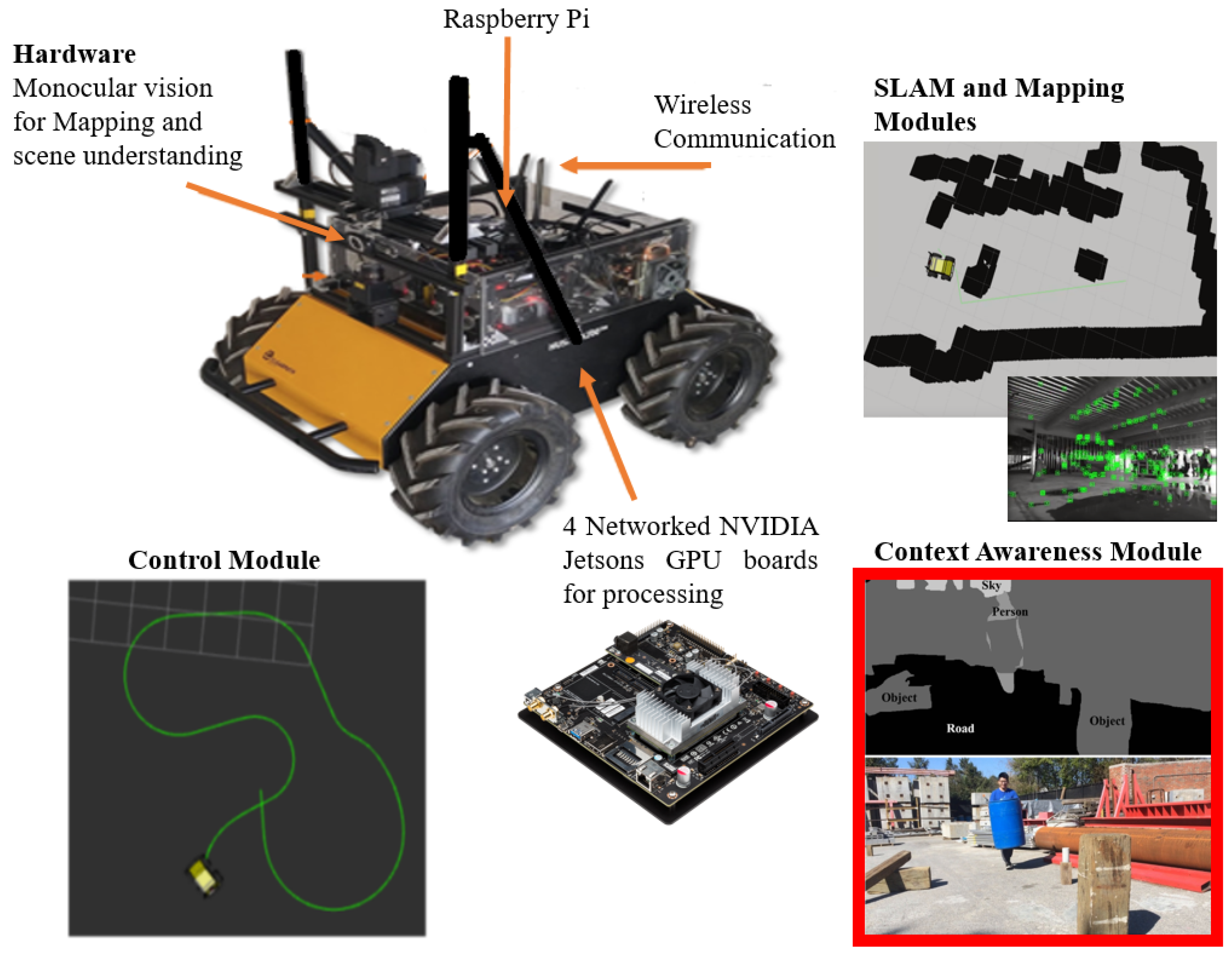
The authors’ previous research on an integrated mobile robotic system [13] presents an unmanned ground vehicle (UGV) that runs multiple modules and enables future development of an autonomous UGV. The platform was built on the Clearpaths Husky mobile robotic platform [14] by incorporating a stack of NVIDIA Jetson TX1 boards (denoted as Jetson boards) [15] and a monocular camera (i.e., a webcam) as a visual sensor. The Jetson boards are low-power embedded devices with integrated Graphics Processing Units (GPUs). In [13], they are used to process simultaneous localization and mapping, motion planning and control, and context awareness (via semantic image segmentation) modules of the system as illustrated in Figure 1.
The two major bottlenecks of this platform, in terms of computational loads, were SLAM and segmentation. For this reason, there was a designated Jetson board for each of these tasks. This is a major challenge in developing an autonomous robot because it increases the size and weight, especially with added batteries. Moreover, the problem becomes even more challenging if this robotics system was to be applied to an unmanned aerial vehicle (UAV).
This previous work implemented ENet [16] as the semantic segmentation method. This segmentation task (shown as Context Awareness Module in the red box in Figure 1) had the heaviest computational load. The inference speed for the ENet implementation on the Jetson TX1, before integration between multiple modules (SLAM, Control, and Context-Awareness each running on a Jetson), for images with the resolution of , was around 15fps. After integration via a wired network the inference rate reduced to 3fps. Data transformation between modules over the network using Robotic Operation System (ROS) [17] caused this slowdown which made the authors restrict the speed of the UGV for real-time performance necessity. Combining the SLAM and Context-Awareness Modules into the same Jetson TX1 would help to mitigate this problem, but the large size of the segmentation model and the high memory usage, make this solution practically unfeasible. Improving the segmentation model in order to reduce the computational load in the Context Awareness Module will address this issue.
2. Research Objectives and Contributions
The major goal of this paper is to propose a deep convolution neural network (CNN) which reduces the computational load (model size) in order to reduce the latency by running multiple modules on the same Jetson. Since Asadi et al. [13] have already validated ENet implementation on the embedded platform in real-time, this paper focuses on comparing the performance of ENet and the proposed method on a server with the following specification: 128 GB RAM, Intel Xeon E5 processor, and two GPUs - NVIDIA Tesla K40c and Telsa K20c.
The ultimate goal is to develop a robotics platform that navigates on construction sites. The hardware development (the authors’ previous work [13]) and algorithm development (this paper) were tailored to navigation on construction sites. This paper proposes a segmentation method to be efficient while providing accurate semantic segmentation.
The main contributions of this paper are (1) creating a new pixel-level annotated dataset for real-time and mobile semantic segmentation in construction environments to deal with the limited number of training dataset and (2) proposing an efficient semantic segmentation method with a smaller model size and faster inference speed for future development of autonomous robots on construction sites. Although the focus of this study is on reducing the model size to enable running multiple modules on the same Jetson TX1, the inference time is also decreased, which increases the maximum input frame rate of the segmentation process for real-time performance.
3. Literature Review
3.1. Vision-Based Object Recognition in Construction
A construction project involves diverse materials, a range of equipment, and a variety of workers, creating a complex and dynamic environment to be predicted. Nowadays, digital cameras are widely used to record construction scenes. Besides increasing the frequency of collecting data, they have reduced the price for acquiring and maintaining the construction-site images [18]. By processing these images properly, the abundant project information can be effectively extracted, which provide an opportunity for automation in construction monitoring.
To process visual data, the first step to be taken is to identify construction objects of interest. To achieve this goal, computer vision is widely used for various construction applications and also has a great potential to automate construction management processes [10,19]. In particular, the characterization of construction resources (i.e., personnel, equipment, and materials) has been one of the major areas that image processing is successfully applied. Many studies have focused on detecting equipment, workers, vehicles, and specific types of construction damages such as cracks in concrete and steel surfaces [20,21,22,23,24,25,26,27,28,29,30,31,32,33].
Park and Brilakis [24] proposed a method to detect construction worker in video frames. The method exploited motion, shape, and color features to characterize workers. Escorcia et al. [25] presented a method that detected construction workers and their actions using colors and depth information from a Microsoft Kinect sensor. They extracted meaningful visual features based on the estimated body pose of workers. Memarzadeh et al. [26] used histograms of oriented gradients and colors for detecting construction workers and equipment from site video streams. Chao and Gay [27] demonstrated a rapid method to recognize and register dynamic heavy equipment operations in 3D views. Their method extracted and processed the target objects’ point cloud data from the background scene and registered 3D target models from a model database to the corresponding point clouds. Park and Brilakis [29] presented a hybrid method to locate construction workers. This method fused tracking and detection together throughout the tracking process. Zhu et al. [28] proposed a framework that integrated the visual tracking into the detection of the construction workforce and equipment. Like the above mentioned methods, in the structural health monitoring studies, deep convolutional neural networks are widely used for detecting civil infrastructure defects to partially replace human-conducted onsite inspections [30,31,32,33].
Similarly, many researchers have conducted research on vision-based material recognition to aid automation in construction progress monitoring [19,34,35,36,37,38,39,40]. Wu et al. [35] proposed a method to extract the objects of interest from construction images using solid imaging algorithms and 3D computer-aided design. Han and Golparvarfard [37] and Han et al. [41] presented geometry and appearance-based material classification methods for monitoring construction progress deviations at the operation level. The method leveraged 4D Building Information Models (BIM) and 3D point cloud models. Kim et al. [19] demonstrated the data-driven scene parsing method to recognize various objects on a construction image. Hamledari et al. [38] proposed a method to detected the components of an interior partition and infer its current state using 2D digital images.
Some of the aforementioned methods were designed for real-time performance. For instance, the construction worker detection method proposed by Park and Brilakis [24] can achieve near real-time (5 fps) performance. However, these methods generally could not provide enough information for construction site navigation. On the other hand, the other data-driven scene parsing methods like the one proposed by Kim et al. [19] are computationally expensive and cannot run on a light-weight embedded device, even equipped with an onboard GPU like NVIDIA Jetson.
3.2. State-of-the-Art Object Recognition
Object recognition has been and still is, one of the major topics of interest in the computer vision community. Object recognition can be performed through object classification or scene segmentation. While semantic segmentation is computationally more intensive for real-time applications, it would result in more accurate boundaries of the objects in the scene, which is more suitable for obstacle avoidance. For instance, object recognition would classify all objects in the scene using boxes whereas semantic segmentation will divide the scene by putting boundaries around the objects. The latter can potentially help the mapping part of the SLAM for a robot.
Even though the technique involving convolutional neural networks (CNN) have been around for years [42], it has not been used for segmentation until recently. Girshik et al. [43] and Girshik [44] combined an image region proposal scheme with CNN as a classifier and performed near real-time inference. CNN-based frameworks for semantic segmentation have also achieved near real-time inference time although the common drawback still is the computational load. On the other hand, Long et al. [45] proposed a semantic segmentation method that took exiting deep CNNs [46,47,48] into a fully convolutional network (FCN) and performed segmentation from their learning representations. Badrinarayanan et al. [49] proposed a semantic segmentation method that was based on a very large encoder-decoder model, performing pixel-wise labeling and resulting in a very large number of computations.
The ability to perform pixel-wise semantic segmentation in real-time is necessary for mobile applications. The above studies have the disadvantage of requiring a large number of floating point operations and have long run-times that hinder their usability. To address this issue, computationally lighter convolutional networks have been presented in [16,50]. In the authors’ previous work [13], for the segmentation model to work on the Jetson board with the limited memory and processing power, ENet [16] which has a smaller architecture compared to the recent deep neural networks was implemented on the UGV. However, the model size and high memory usage of this model forced the authors to allocate a separate Jetson to this module. The resulting latency in data transformation between different modules, caused by integrating multiple Jetson through the network, made the system inefficient in fast movements. This latency forced the authors to restrict the speed of the UGV for real-time performance necessity. Therefore, one of the two main contributions of this paper focuses on proposing a new segmentation model by reducing the model size and memory usage while maintaining accuracy.
4. Method
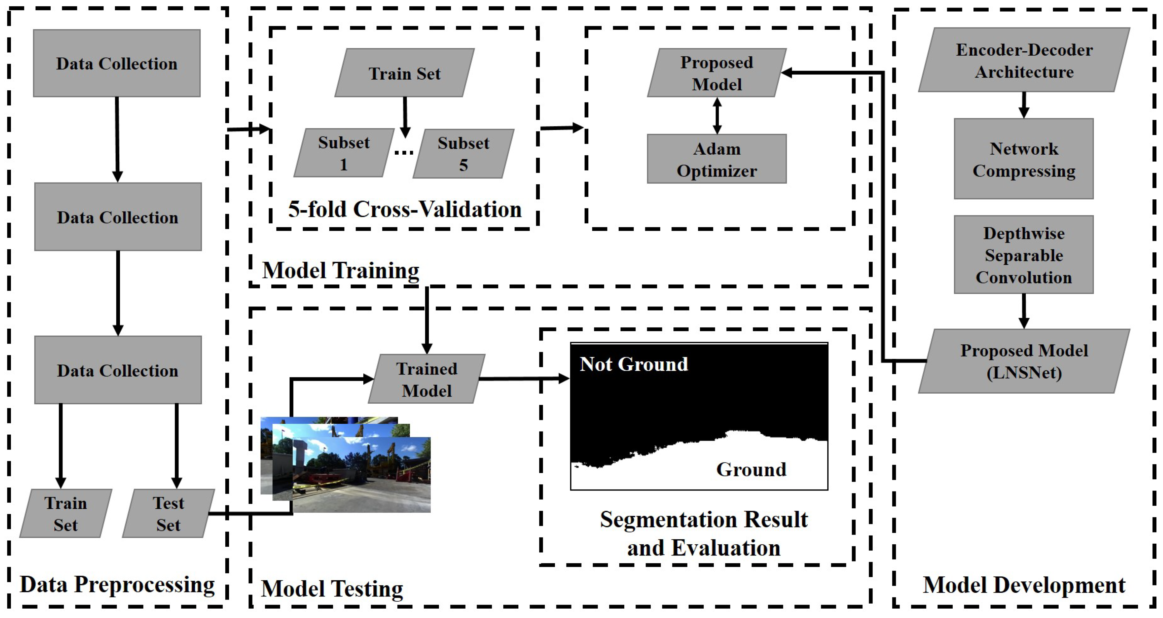
Real-time semantic segmentation algorithms are used to understand the content of images and find target objects in real-time which are crucial tasks in mobile robotic systems. In the computer vision fields, there is a growing interest in the use of deep neural network techniques for semantic segmentation tasks. In this part, a new convolutional neural network model architecture, namely LNSNet, as well as the strategies and techniques for its training, compressing and data processing will be introduced. Adam Optimizer [51] is used to train the model and cross-entropy is utilized as loss function. Also, a new pixel-level annotated dataset has been generated and validated for real-time and mobile semantic segmentation in a construction engineering environment. Figure 2 shows an overview of the components of the proposed algorithm. Each step is discussed in the following subsections.
4.1. Model Architecture
In this section, firstly, factorized convolution block as a core block is described which LNSNet is built on. Then the LNSNet network structure is illustrated followed by a model compressing method description.
4.1.1. Factorized Convolution Block
To optimize the amount of parameters in a CNN model while maintaining its performance, cut down the model sizes, and run the model faster, Depthwise Separable Convolution from MobileNet [50] is applied. Depthwise Separable Convolution is a form of factorized convolutions which factorizes a standard convolution into two separate operations—a depthwise convolution and a point-wise convolution. While the standard convolution operates over every channel of the input feature map, Depthwise Separable Convolution applies a single filter on every channel and use a point-wise convolution, () kernel convolution, and linearly combines the outputs. For a standard convolution layer whose kernel size is K, it takes a feature map of size as input where , , are height, width, and channels respectively, and outputs a feature map of size . The computational cost is computed using Equation (1).
Equation (2), shows the computational cost for separable depthwise convolution, considering the same feature map.
By transforming the original convolution operation into depthwise separable convolution, the reduction in computation cost is calculated by Equation (3)
In the proposed method, depthwise separable convolutional layers replace the standard convolution layers in a CNN model. This replacement reduces computational cost. For instance, a convolutional layer with filters is substituted with depthwise separable convolutional layer. The reduced computational cost is 0.13 which means that the model uses almost 8 times less computation than standard computations which means that the model uses almost 8 times less computation than standard computations (see Equation (4)).
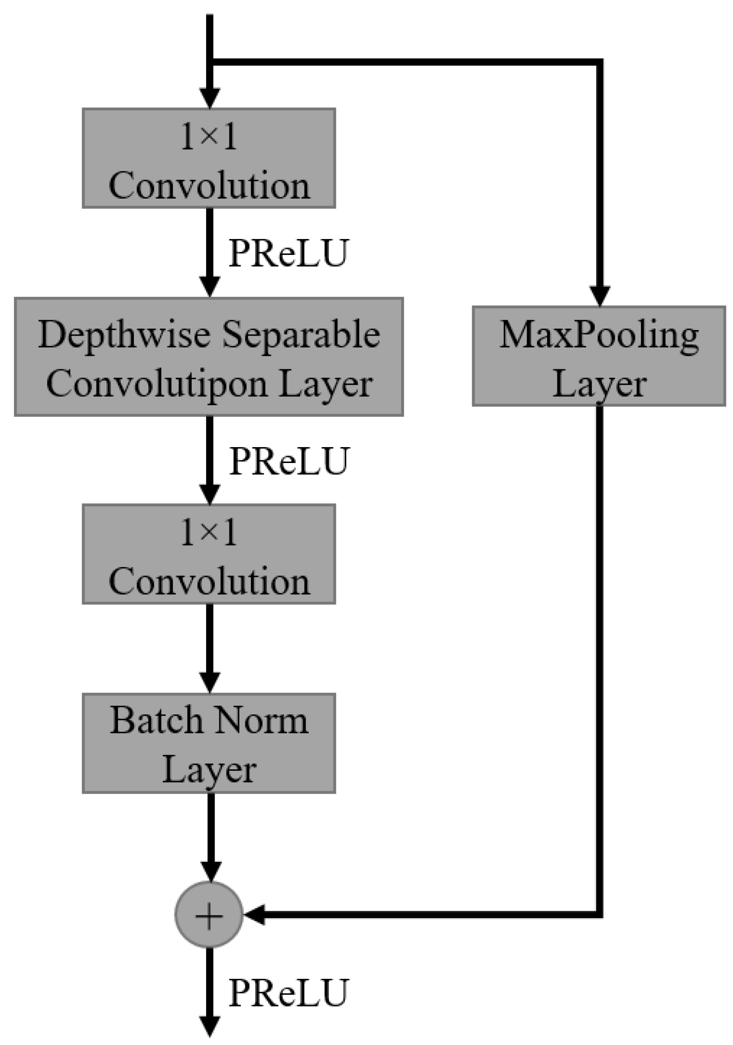
By utilizing the strength of depthwise separable convolution, we proposed a new residual block based on the traditional residual block. The block has two branches. One branch consists of two convolutional layers (the first one is for projection and reducing the dimensionality which is located before the depthwise separable convolution layer and the second one is placed afterward which is for expansion), a depthwise convolutional layer, and a batch normalization layer at the end. The other one is a shortcut branch which outputs an identical feature map as its input. If the type of the block is Downsample, a MaxPooling layer is added to the shortcut branch. At the end of the block, the outputs from the two branches are element-wise added. The structure of the block is shown in Figure 3.
4.1.2. Architecture Design
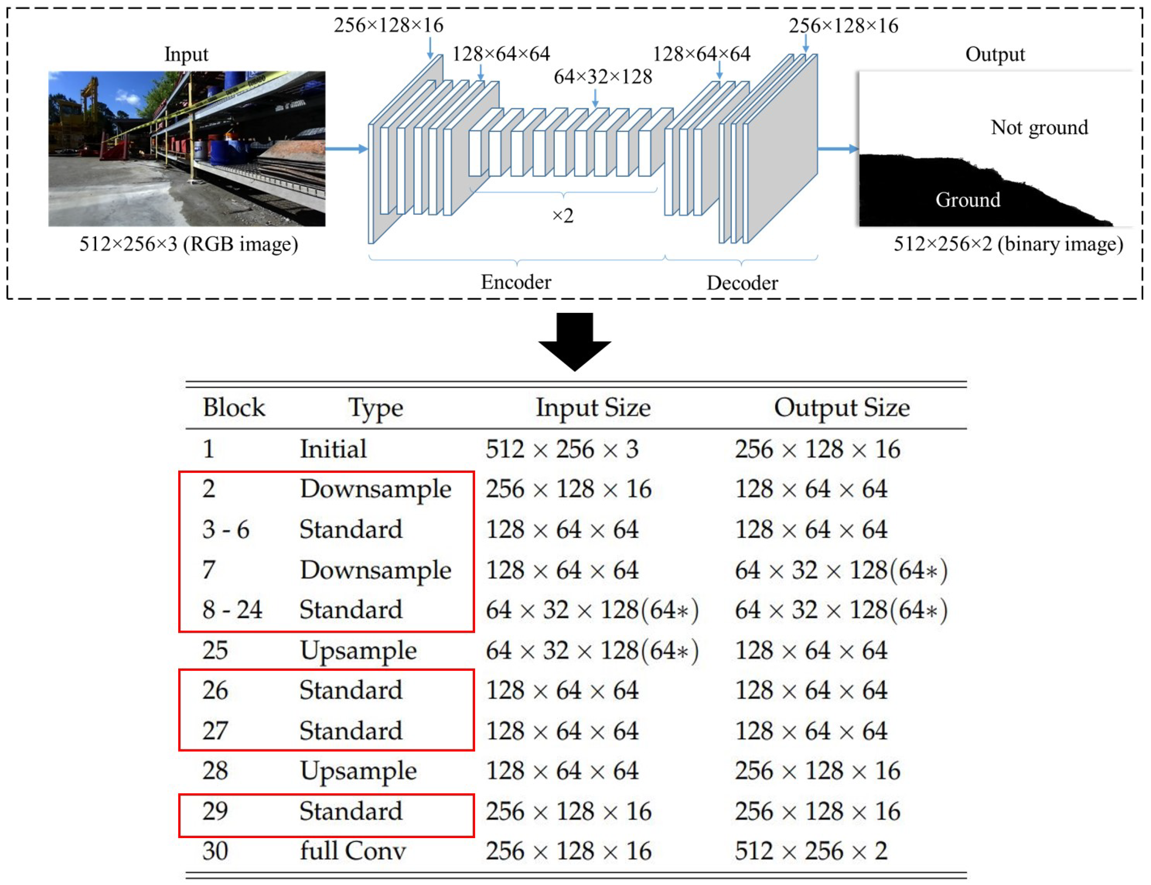
The proposed method has a light model that has been optimized for a mobile device and real-time semantic segmentation applications. Moreover, the algorithm needs two classes (i.e., navigable space and non-navigable space) for classifying open spaces for navigation and mapping. LNSNet has an encoder-decoder architecture, which consists of several Factorized Convolution Blocks. The architecture of our network is presented in Figure 4.
In the first Initial block where we followed the ENet architecture, we concatenated the output of a convolutional layer with the stride of two and a MaxPooling layer to decrease the feature size at an early stage. The Downsample and Standard blocks follow the structure we illustrated in the Factorized Convolution Block part. As for the Upsample and LastConv blocks, the same configurations are applied as ENet. The channels indicated by the * sign in Figure 4, originally designed to be 128; however, they compressed to 64 by model compression (to be further detailed in the following section)
4.1.3. Model Compressing
A well-trained CNN model usually has significant redundancy among different filters and feature channels. Therefore, an efficient way to cut down both computational cost and model size is to compress the model [52].
For a layer whose kernel size is K, it transforms an input feature map into an output feature map whose shape is . The shape of the kernel matrix is . Each single filter in the kernel could generates one layer of the output feature map. norm of the filter is used to evaluate the efficiency of the filter. The norm of a vector x is calculated using Equation (5), where represents each value of the kernel.
If the norm is close to zero, it generates negligible output because the output feature map values tend to be close to zero. To improve efficiency, removing these filters would reduce the computational expense and model size. After removing the filters, the corresponding output feature map channels would also be removed.
Network compressing consists of the following steps:
- (1)
- For each filter, calculate the value.
- (2)
- Sort filters by values calculated in Step1.
- (3)
- Remove the filters and corresponding feature maps.
- (4)
- Fine-tune the whole network.
Since the architecture of LNSNet is much more complex compared to CNNs without residual connections, such as AlexNet [47] and VGG [48], the first several layers are very sensitive and could have a huge impact on the layers behind and the overall performance.
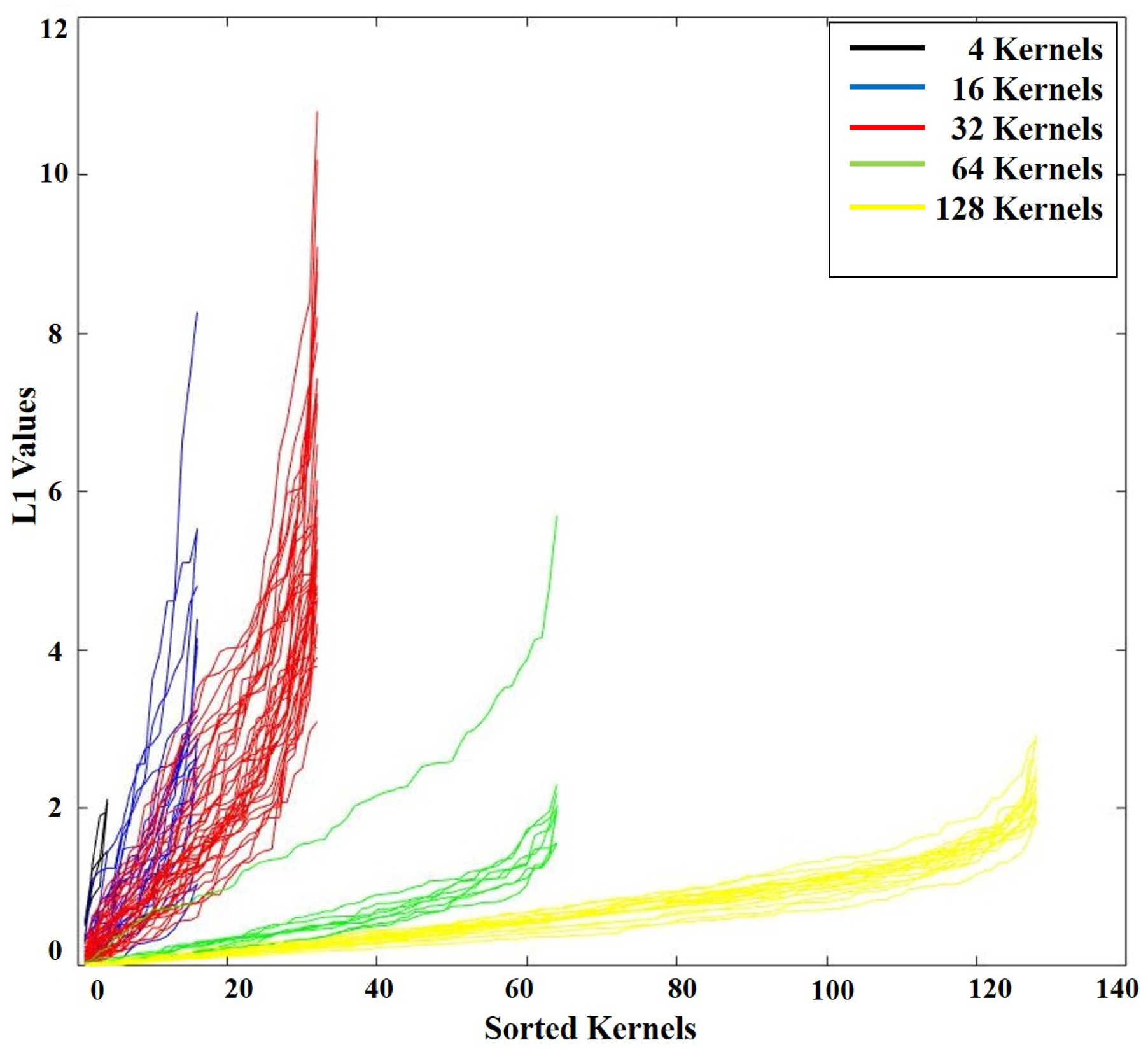
However, it is hard to predict how many filters and which filters can be removed without damaging the performance. As shown in Figure 5, by calculating and sorting the values of every filter in the model, the 128 filters (denoted as 128-kernels) generally have smaller values and have the largest number of redundant filters. 128-kernels are less sensitive to the changes compared to other kernels. Therefore, removing 128-kernels have a negligible impact on performance. As shown in Figure 5, the values for half of them is less than one, which indicates that they have a small impact on the overall performance. As a result, these filters could be removed without harming the accuracy. As it is shown in Figure 4 half of the filters of 128-kernels are removed (is indicated with * in the figure) and the model is fine-tuned on the same dataset.
4.2. Optimizer and Loss Function
The Adam algorithm [51] is implemented as an optimization method. This method is based on adaptive estimates of lower-order moments and is designed for first-order gradient-based optimization of stochastic objective functions. A learning rate of 0.1 is used with = 0.9 and = 0.999. and are exponential decay rates for the moment estimates. For the loss function, binary cross entropy is applied for binary segmentation task. The cross entropy is given by Equation (6).
Cross-entropy can be used as an error measure if the outputs of the last layer of a neural network are treated as probabilities. In Equation (6), p is the true distribution of the possibilities of the classifications. On the other hand, q is the predicted distribution of the possibilities which are from the network’s output. Cross-entropy can represent the likelihood of true and predicted distributions. As for binary cross-entropy, the loss function used in the method is a special case of the general cross-entropy when the number of classes is two.
5. Experimental Setup
5.1. Dataset Construction and Training Strategy
A new dataset has been constructed for the proposed method. The main objective of our classification task is to segment all objects from navigable spaces in the scene, which is why the proposed method has only two classes. To segment objects even in a new environment, the data is collected from three completely different environments including construction sites, parking lots, and roads (1000 images).
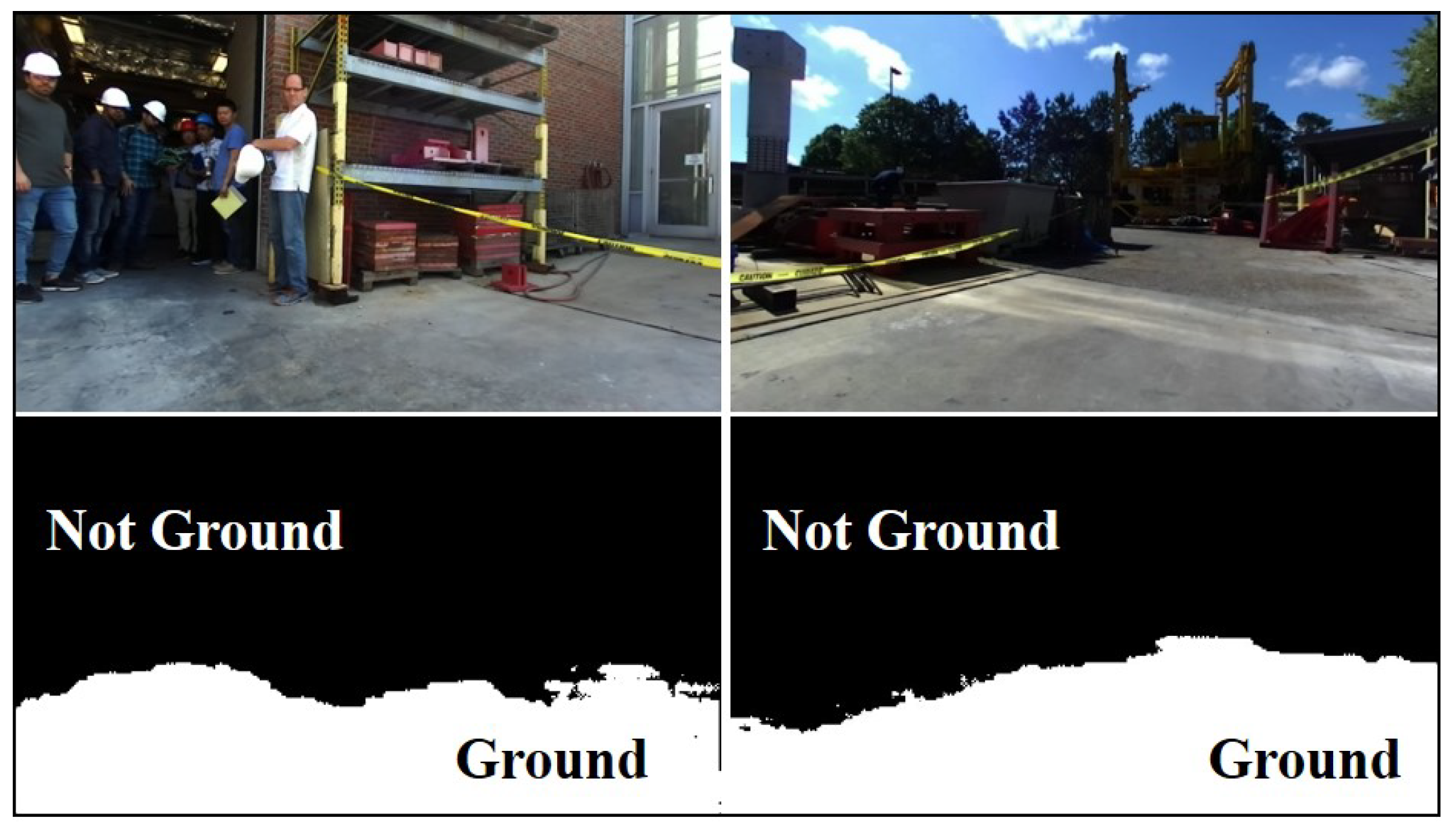
Images from the new dataset are collected with the following considerations: First, the angle of the camera is varied randomly for the training data. Second, images are collected in different weather conditions. Third, only two labels are assigned to the pixels during annotation; Ground and Not Ground. This strategy highly simplified the labeling task while still addressing a fundamental requirement for autonomous navigation (i.e., the identification of drivable terrain by the autonomous agent).
In addition, an updated Cityscapes public dataset [53] is also used for training and testing process. This dataset can prevent over-fitting of the proposed model. Therefore, it was used for training and cross-validation. Cityscape has 5000 frames that have high-quality pixel-level annotations. As it has 30 classes, these labels are grouped into 2 classes for our task. Table 1, shows the strategy used for grouping the labels. Both Cityscapes and the newly collected datasets are combined in later experiments. All images that were used have been resized to pixels. Figure 6 (top), shows a sample images from new dataset and Figure 6 (bottom) is their corresponding labels.
Since Asadi et al. [13] have already validated ENet implementation on the embedded platform in real-time, this paper focuses on comparing the performance of ENet and the proposed method on a server with the following specification: 128 GB RAM, Intel Xeon E5 processor, and two GPUs-NVIDIA Tesla K40c and Telsa K20c.
Tensorflow [54] and Keras [55] framework are used to implement the algorithm. CUDA [56] and CuDNN [57] are also utilized for accelerating the computations. The whole training process took about 12 h. The batch size is an important parameter in deep learning. A small batch size typically makes the model hard to converge. Large batch size can increase the efficiency by parallel computing and make full use of memory [58]. On the other hand, a large batch size would also cause a huge demand for memory. A batch size of 32 has been used in training. During each step, one batch is used for training. The total step is 200 per epoch. For each epoch, the training program runs through the whole dataset once. The total number of epochs is 15.
The training data is K-fold cross-validated by dividing it into K subsets [59]. Each time, one of the subsets is used as the validation set and the rest is used as the training set. Every data is used times for training and one time for validation. For this experiment, K is set to five. The validation set is used after each epoch of training in order to evaluate accuracy and loss.
5.2. Data Augmentation
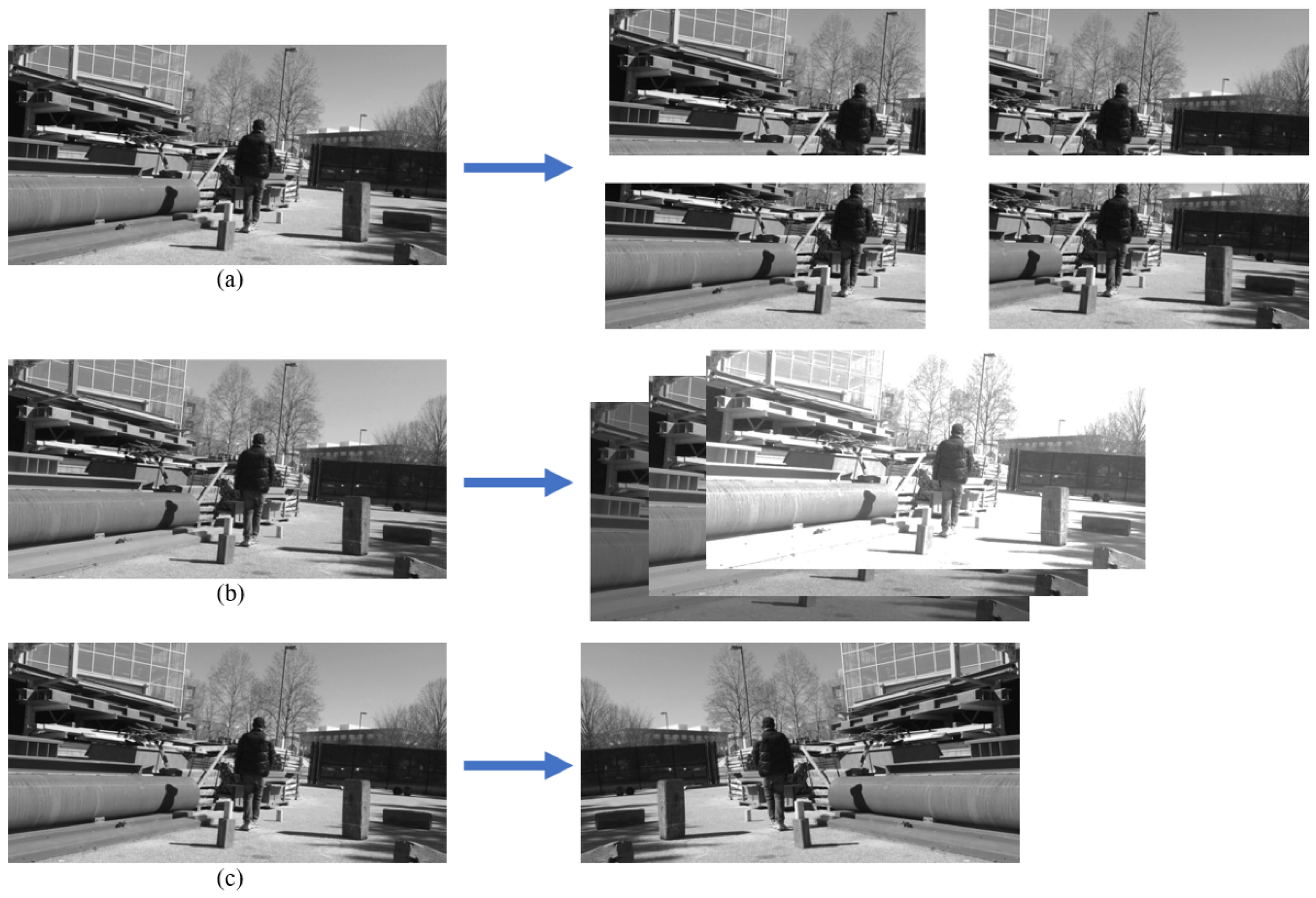
Deep learning models need to be trained on a large dataset. A small data set could cause over-fitting (i.e., performing well on the training data but not on the testing data). To deal with this challenge of having a limited number of the training images, label-preserving data augmentation is used. In this research similar to krizhevsky et al. [47], different methods of data augmentation such as random cropping, random color jitter, and flipping are implemented (see Figure 7).
Random cropping randomly selects a smaller region of the raw image, along with its corresponding annotation—therefore, “label-preserving” as mentioned previously. Then the region is resized to the raw image size and considered as a new sample. Random cropping utilizes the translation-invariance feature of the object in the dataset (see Figure 7a. Random color jitter makes a slight change in the color values of the image. The purpose of this operation is to simulate and generate different lighting conditions (see Figure 7b. A gamma correction function has been used as the Equation (7) shows. is the color value of every pixel in the input images. is the value in the output images, corresponding to the input images pixel by pixel. This equation randomly chooses the parameter from 0.5 to 1.5 for each image. Finally, regarding Figure 7c, flipping flips the images horizontally. These three methods are also applied simultaneously to generate more samples. During training, making data regularized is a common trick in deep learning, and gray-scale images are rescaled from 0–255 to 0–1. Each image in the original dataset could generate 32 new images through this data augmentation approach.
6. Experimental Results
6.1. Training Results
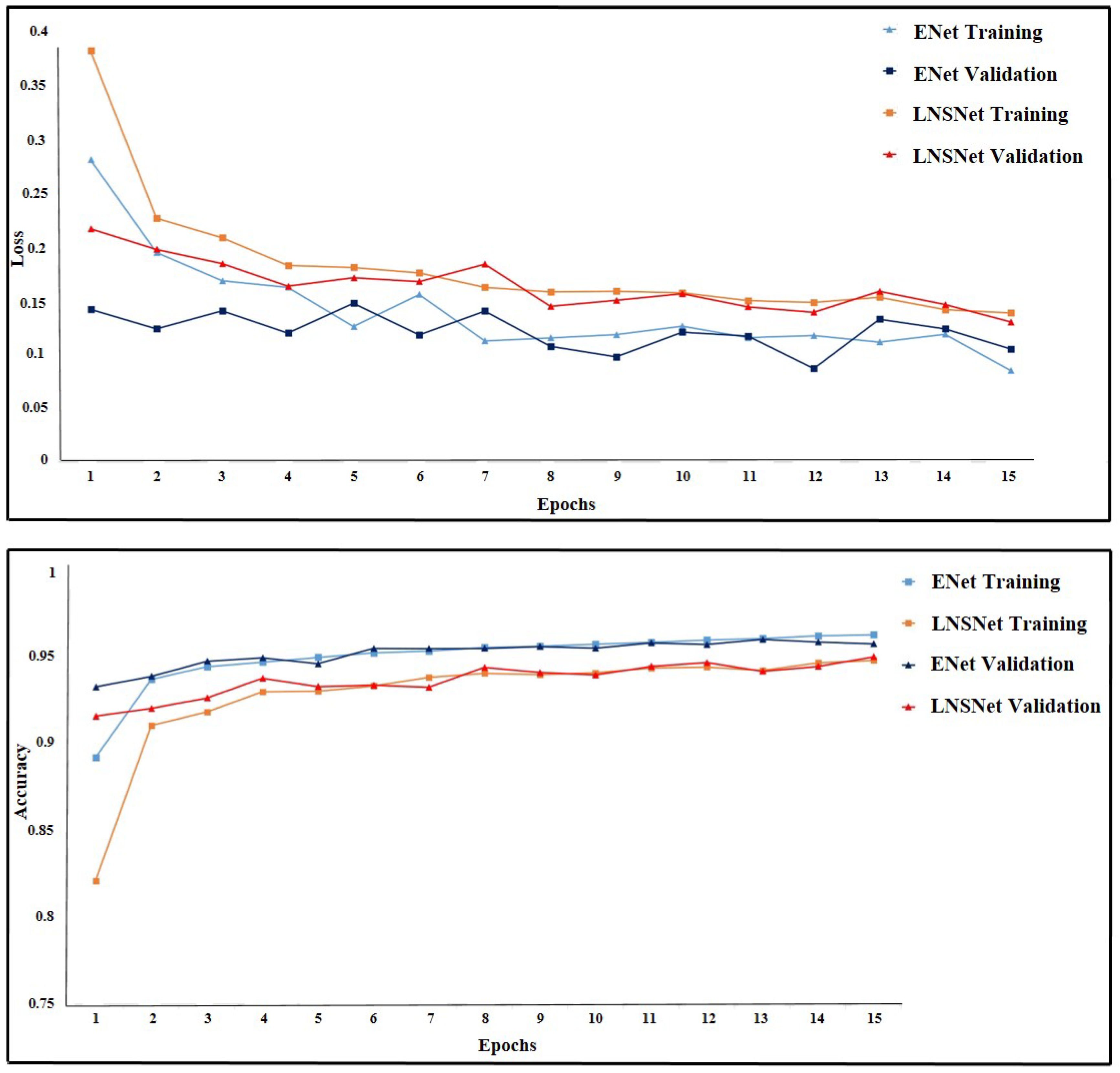
Figure 8 (bottom) shows the relations between accuracy and epochs during the training of both ENet and LNSNet models. Each line in the figure represents the average loss or accuracy of all splits during cross-validation. As the loss function decreases, the accuracy of the model increases, showing that the segmentation ability of the model is elevated. Figure 8 (top) shows variations in losses while training. The loss or cross-entropy in the figure decreases when the predictions are more accurate.
Since there is no obvious depart between validation loss and training loss, there is no over-fitting in the training. As the first validation is conducted after the first epoch of training, the model has already improved the classification ability at that time. On the other hand, the first point of training lines shows the model accuracy right after the initialization. So, the validation curves always start from a relatively higher accuracy than the training curves. Table 2 shows accuracy, precision, and recall rates at the end of the training process for both ENEt and LNSNet models.
6.2. Test Results
For testing and evaluation, 150 images are used from three scenes, including a parking lot, road, and construction site. Due to the differences between the three scenes, models performance is varied and highly related to the complexity of images and categories of objects. The test results are shown in Table 3.
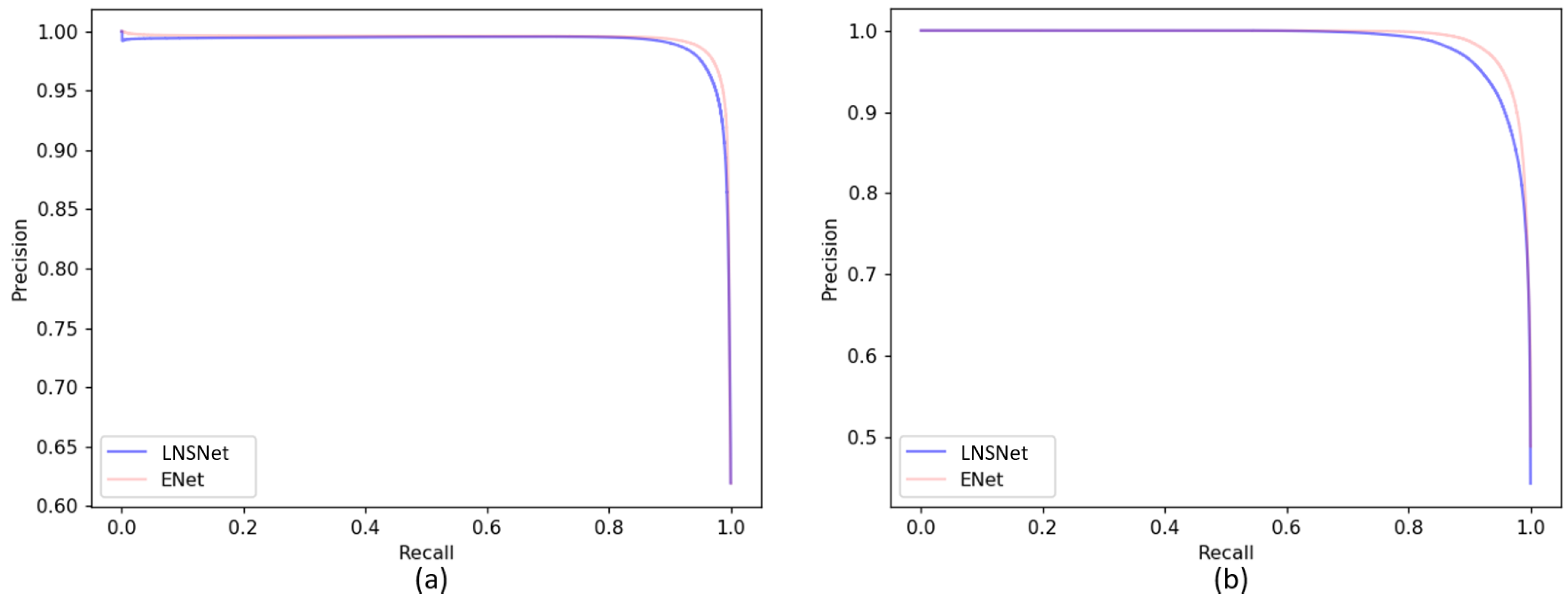
A precision-recall curve is also drawn to evaluate the two models. Figure 9 shows the relation between precision and recall while changing the thresholding value of the binary classification. As it is shown in Figure 9, Table 2 and Table 3, the LNSNet model has almost similar accuracy, precision, and recall rates rates compare to those of ENet. The difference was around 2% and the precision-recall curves are approximately overlapped, indicating no significant difference in accuracy.
6.3. Model Comparison
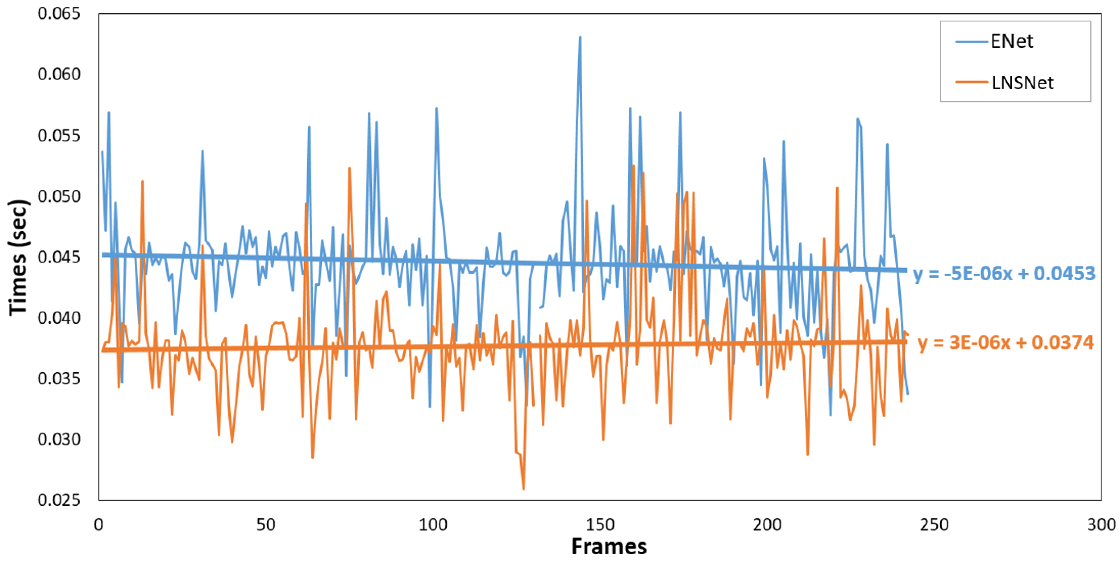
The results in Table 2 and Table 3 show that only 2% percent of accuracy is lost, on the other hand, the complexity of the network is reduced greatly by decreasing the parameters and the feature layers by half. The model size drops from 2225 KB to 1068 KB. The comparison between the two models is shown in Table 4. The inference time is directly related to computation cost in the network. The proposed model’s inference time decreased about 18%, although the number of parameters decreased significantly (see Table 4 and Figure 10). There are two tasks performed by the GPU: creating the kernel and evaluating the model. The proposed model only decreases the evaluation time which is why the inference time does not decrease at the same rate. In other words, the inference time depends greatly on other computation factors rather than just the evaluation of the neural network model (i.e., the cost of launching the GPU kernel starts to dominate the computation time).
Table 5 shows the means, standard deviations, and t-test results which indicate that the average inference time per frame has reduced from 44.7 ms to 36.5 ms per frame. This reduction in the inference time means that the maximum input frame rate for real-time performance can be increased by 5 fps (from 22 fps in ENet to 27 fps in LNSNet). The p-value of indicates that the difference is statistically significant at = 0.01. Although the proposed segmentation method has a lower inference time compare to the ENet method, the main contribution of the proposed method is reducing the model size (more than 50%). This reduction enables multiple modules to be run on the same Jetson TX1, which will reduce the latency caused by integrating multiple Jetson TX1s through the wired network.
7. Conclusions and Future Works
One of the major challenges in a robotic system that integrates multiple modules on a single modular framework, is the integration between the modules which are running on separate processing units. Latency in data transformation between different processing units decreases the performance of the system. Combining modules to run on the same processing unit can address this challenge and also reduces the cost, size, and weight of the system which counts as a significant improvement for mobile robotic systems that have either limited computing resources or payload capacity (e.g., unmanned aerial vehicles). This paper presents an efficient semantic segmentation model that can be run in real-time on multiple embedded platforms that are integrated as a system to determine navigable space in real-time. The results show improvement in model size, memory usage, and computation time (50% and 18% reduction in model size and inference time respectively) while keeping the accuracy almost the same. 50% reduction in the model size is a significant contribution, which enables multiple modules to be combined and run on the same processing unit. The core of model architecture is a new block based on separable convolution which compresses the parameters of present residual block meanwhile maintaining the accuracy and performance.
The proposed method is a step forward in making intelligent and contextually aware robots ubiquitous. In the future, the model’s segmentation ability and inference speed could be further improved by applying new neural network architectures and new loss function design. The proposed binary problem in the dataset is a good starting point but more complex classification tasks would be required in more realistic scenarios. So, a high-precise and multi-class annotated construction site dataset are in need. Moreover, existing 3D models (i.e., BIM) of construction sites can potentially guide and streamline the data collection of highly precise pixel-level annotations.
Author Contributions
Conceptualization, K.A. and P.C. and K.H.; methodology, K.A. and P.C. and K.H.; software, K.A. and P.C.; validation, K.A. and P.C. and K.H.; formal analysis, K.A. and P.C.; investigation, K.A. and P.C.; resources, K.H. and T.W. and E.L.; data curation, K.A. and P.C.; writing—original draft preparation, K.A. and P.C. and K.H.; writing—review and editing, K.A. and P.C. and K.H. and T.W. and E.L.; visualization, K.A. and P.C. and K.H.; supervision, K.A. and K.H.; project administration, K.A. and K.H.
Funding
This research received no external funding.
Acknowledgments
The authors gratefully acknowledge the support of NVIDIA Corporation with the donation of the Tesla K40 Graphics Processing Units used for this research. Any opinions, findings, conclusions or recommendations presented in this paper are those of the authors and do not reflect the views of NVIDIA.
Conflicts of Interest
The authors declare no conflicts of interest.
References
- Changali, S.; Mohammad, A.; van Nieuwl, M. The Construction Productivity Imperative; McKinsey & Company: Brussels, Belgium, 2015. [Google Scholar]
- Kangari, R.; Yoshida, T. Automation in construction. Robot. Auton. Syst. 1990, 6, 327–335. [Google Scholar] [CrossRef]
- Chan, A.P.; Scott, D.; Chan, A.P. Factors affecting the success of a construction project. J. Construct. Eng. Manag. 2004, 130, 153–155. [Google Scholar] [CrossRef]
- Asadi, K.; Ramshankar, H.; Noghabaee, M.; Han, K. Real-time Image Localization and Registration with BIM Using Perspective Alignment for Indoor Monitoring of Construction. J. Comput. Civ. Eng. 2019. [Google Scholar]
- Han, K.K.; Golparvar-Fard, M. Potential of big visual data and building information modeling for construction performance analytics: An exploratory study. Autom. Constr. 2017, 73, 184–198. [Google Scholar] [CrossRef]
- Asadi, K.; Ramshankar, H.; Pullagurla, H.; Bhandare, A.; Shanbhag, S.; Mehta, P.; Kundu, S.; Han, K.; Lobaton, E.; Wu, T. Building an Integrated Mobile Robotic System for Real-Time Applications in Construction. arXiv, 2018; arXiv:1803.01745. [Google Scholar]
- Asadi, K.; Han, K. Real-Time Image-to-BIM Registration using Perspective Alignment for Automated Construction Monitoring. In Construction Research Congress 2018, New Orleans, LA, USA, 2–4 April 2018; ASCE: Reston, VA, USA, 2018; pp. 388–397. [Google Scholar]
- Kropp, C.; Koch, C.; König, M. Interior construction state recognition with 4D BIM registered image sequences. Autom. Constr. 2018, 86, 11–32. [Google Scholar] [CrossRef]
- Asadi Boroujeni, K.; Han, K. Perspective-Based Image-to-BIM Alignment for Automated Visual Data Collection and Construction Performance Monitoring. In Computing in Civil Engineering 2017, Seattle, WA, USA, 25–27 June 2017; ASCE: Reston, VA, USA, 2017; pp. 171–178. [Google Scholar]
- Yang, J.; Park, M.W.; Vela, P.A.; Golparvar-Fard, M. Construction performance monitoring via still images, time-lapse photos, and video streams: Now, tomorrow, and the future. Adv. Eng. Informat. 2015, 29, 211–224. [Google Scholar] [CrossRef]
- Ham, Y.; Han, K.K.; Lin, J.J.; Golparvar-Fard, M. Visual monitoring of civil infrastructure systems via camera-equipped Unmanned Aerial Vehicles (UAVs): A review of related works. Vis. Eng. 2016, 4, 1. [Google Scholar] [CrossRef]
- Liu, P.; Chen, A.Y.; Huang, Y.N.; Han, J.Y.; Lai, J.S.; Kang, S.C.; Wu, T.; Wen, M.; Tsai, M. A review of rotorcraft unmanned aerial vehicle (UAV) developments and applications in civil engineering. Smart Struct. Syst. 2014, 13, 1065–1094. [Google Scholar] [CrossRef]
- Asadi, K.; Ramshankar, H.; Pullagurla, H.; Bhandare, A.; Shanbhag, S.; Mehta, P.; Kundu, S.; Han, K.; Lobaton, E.; Wu, T. Vision-based integrated mobile robotic system for real-time applications in construction. Autom. Constr. 2018, 96, 470–482. [Google Scholar] [CrossRef]
- ClearPathRobotics. husky-unmanned-ground-vehicle-robot. Available online: https://www.clearpathrobotics.com/husky-unmanned-ground-vehicle-robot/ (accessed on 29 November 2017).
- NVIDIA. Unleash Your Potential with the Jetson TX1 Developer Kit. Available online: https://developer.nvidia.com/embedded/buy/jetson-tx1-devkit (accessed on 29 November 2017).
- Paszke, A.; Chaurasia, A.; Kim, S.; Culurciello, E. ENet: A Deep Neural Network Architecture for Real-Time Semantic Segmentation. CoRR, 2016; arXiv:1606.02147. [Google Scholar]
- Quigley, M.; Gerkey, B.; Conley, K.; Faust, J.; Foote, T.; Leibs, J.; Berger, E.; Wheeler, R.; Ng, A. ROS: An open-source Robot Operating System. In Proceedings of the IEEE International Conference on Robotics and Automation (ICRA) Workshop on Open Source Robotics, Kobe, Japan, 12–17 May 2009. [Google Scholar]
- Golparvar-Fard, M.; Peña-Mora, F.; Savarese, S. D4AR–a 4-dimensional augmented reality model for automating construction progress monitoring data collection, processing and communication. J. Inf. Technol. Construct. 2009, 14, 129–153. [Google Scholar]
- Kim, H.; Kim, K.; Kim, H. Data-driven scene parsing method for recognizing construction site objects in the whole image. Autom. Constr. 2016, 71, 271–282. [Google Scholar] [CrossRef]
- Brilakis, I.; Park, M.W.; Jog, G. Automated vision tracking of project related entities. Adv. Eng. Informat. 2011, 25, 713–724. [Google Scholar] [CrossRef]
- Teizer, J.; Vela, P. Personnel tracking on construction sites using video cameras. Adv. Eng. Informat. 2009, 23, 452–462. [Google Scholar] [CrossRef]
- Yang, J.; Arif, O.; Vela, P.A.; Teizer, J.; Shi, Z. Tracking multiple workers on construction sites using video cameras. Adv. Eng. Informat. 2010, 24, 428–434. [Google Scholar] [CrossRef]
- Chi, S.; Caldas, C.H. Automated object identification using optical video cameras on construction sites. Comput.-Aided Civ. Infrastruct. Eng. 2011, 26, 368–380. [Google Scholar] [CrossRef]
- Park, M.W.; Brilakis, I. Construction worker detection in video frames for initializing vision trackers. Autom. Constr. 2012, 28, 15–25. [Google Scholar] [CrossRef]
- Escorcia, V.; Dávila, M.A.; Golparvar-Fard, M.; Niebles, J.C. Automated vision-based recognition of construction worker actions for building interior construction operations using RGBD cameras. In Construction Research Congress 2012: Construction Challenges in a Flat World; 21–23 May 2012; West Lafayette, IN, USA; ASCE: Reston, VA, USA, 2012; pp. 879–888. [Google Scholar]
- Memarzadeh, M.; Golparvar-Fard, M.; Niebles, J.C. Automated 2D detection of construction equipment and workers from site video streams using histograms of oriented gradients and colors. Autom. Constr. 2013, 32, 24–37. [Google Scholar] [CrossRef]
- Cho, Y.K.; Gai, M. Projection-recognition-projection method for automatic object recognition and registration for dynamic heavy equipment operations. J. Comput. Civ. Eng. 2013, 28, A4014002. [Google Scholar] [CrossRef]
- Zhu, Z.; Ren, X.; Chen, Z. Integrated detection and tracking of workforce and equipment from construction jobsite videos. Autom. Constr. 2017, 81, 161–171. [Google Scholar] [CrossRef]
- Park, M.W.; Brilakis, I. Continuous localization of construction workers via integration of detection and tracking. Autom. Constr. 2016, 72, 129–142. [Google Scholar] [CrossRef]
- Kang, D.; Cha, Y.J. Autonomous UAVs for Structural Health Monitoring Using Deep Learning and an Ultrasonic Beacon System with Geo-Tagging. Comput.-Aided Civ. Infrastruct. Eng. 2018, 33, 885–902. [Google Scholar] [CrossRef]
- Cha, Y.J.; Choi, W.; Suh, G.; Mahmoudkhani, S.; Büyüköztürk, O. Autonomous Structural Visual Inspection Using Region-Based Deep Learning for Detecting Multiple Damage Types. Comput.-Aided Civ. Infrastruct. Eng. 2017, 33, 731–747. [Google Scholar] [CrossRef]
- Gao, Y.; Mosalam, K.M. Deep Transfer Learning for Image-Based Structural Damage Recognition. Comput.-Aided Civ. Infrastruct. Eng. 2018, 33, 748–768. [Google Scholar] [CrossRef]
- Cha, Y.J.; Choi, W.; Büyüköztürk, O. Deep Learning-Based Crack Damage Detection Using Convolutional Neural Networks. Comput.-Aided Civ. Infrastruct. Eng. 2017, 32, 361–378. [Google Scholar] [CrossRef]
- Zhu, Z.; Paal, S.; Brilakis, I. Detection of large-scale concrete columns for automated bridge inspection. Autom. Constr. 2010, 19, 1047–1055. [Google Scholar] [CrossRef]
- Wu, Y.; Kim, H.; Kim, C.; Han, S.H. Object recognition in construction-site images using 3D CAD-based filtering. J. Comput. Civ. Eng. 2009, 24, 56–64. [Google Scholar] [CrossRef]
- Son, H.; Kim, C.; Kim, C. Automated color model–based concrete detection in construction-site images by using machine learning algorithms. J. Comput. Civ. Eng. 2011, 26, 421–433. [Google Scholar] [CrossRef]
- Han, K.K.; Golparvar-Fard, M. Appearance-based material classification for monitoring of operation-level construction progress using 4D {BIM} and site photologs. Autom. Constr. 2015, 53, 44–57. [Google Scholar] [CrossRef]
- Hamledari, H.; McCabe, B.; Davari, S. Automated computer vision-based detection of components of under-construction indoor partitions. Autom. Constr. 2017, 74, 78–94. [Google Scholar] [CrossRef]
- Li, H.; Chan, G.; Wong, J.K.W.; Skitmore, M. Real-time locating systems applications in construction. Autom. Constr. 2016, 63, 37–47. [Google Scholar] [CrossRef]
- Asadi, K.; Jain, R.; Qin, Z.; Sun, M.; Noghabaei, M.; Cole, J.; Han, K.; Lobaton, E. Vision-based Obstacle Removal System for Autonomous Ground Vehicles Using a Robotic Arm. arXiv, 2019; arXiv:cs.RO/1901.08180. [Google Scholar]
- Han, K.; Degol, J.; Golparvar-Fard, M. Geometry- and Appearance-Based Reasoning of Construction Progress Monitoring. J. Construct. Eng. Manag. 2018, 144, 04017110. [Google Scholar] [CrossRef]
- LeCun, Y.; Bottou, L.; Bengio, Y.; Haffner, P. Gradient-based learning applied to document recognition. Proc. IEEE 1998, 86, 2278–2324. [Google Scholar] [CrossRef] [Green Version]
- Girshick, R.; Donahue, J.; Darrell, T.; Malik, J. Rich Feature Hierarchies for Accurate Object Detection and Semantic Segmentation. In Proceedings of the IEEE Conference on Computer Vision and Pattern Recognition (CVPR), Columbus, OH, USA, 24–27 June 2014; pp. 580–587. [Google Scholar]
- Girshick, R. Fast r-cnn. In Proceedings of the IEEE International Conference on Computer Vision, Santiago, Chile, 7–13 December 2015; pp. 1440–1448. [Google Scholar]
- Long, J.; Shelhamer, E.; Darrell, T. Fully convolutional networks for semantic segmentation. In Proceedings of the IEEE Conference on Computer Vision and Pattern Recognition (CVPR), Boston, MA, USA, 7–12 June 2015; pp. 3431–3440. [Google Scholar]
- Szegedy, C.; Liu, W.; Jia, Y.; Sermanet, P.; Reed, S.; Anguelov, D.; Erhan, D.; Vanhoucke, V.; Rabinovich, A. Going deeper with convolutions. In Proceedings of the IEEE Conference on Computer Vision and Pattern Recognition, Boston, MA, USA, 7–12 June 2015; pp. 1–9. [Google Scholar]
- Krizhevsky, A.; Sutskever, I.; Hinton, G.E. Imagenet classification with deep convolutional neural networks. Adv. Neural Inf. Process. Syst. 2012, 25, 1097–1105. [Google Scholar] [CrossRef]
- Simonyan, K.; Zisserman, A. Very deep convolutional networks for large-scale image recognition. arXiv, 2014; arXiv:1409.1556. [Google Scholar]
- Badrinarayanan, V.; Kendall, A.; Cipolla, R. Segnet: A deep convolutional encoder-decoder architecture for image segmentation. arXiv, 2015; arXiv:1511.00561. [Google Scholar] [CrossRef]
- Howard, A.G.; Zhu, M.; Chen, B.; Kalenichenko, D.; Wang, W.; Weyand, T.; Andreetto, M.; Adam, H. Mobilenets: Efficient convolutional neural networks for mobile vision applications. arXiv, 2017; arXiv:1704.04861. [Google Scholar]
- Kingma, D.; Ba, J. Adam: A method for stochastic optimization. arXiv, 2014; arXiv:1412.6980. [Google Scholar]
- Li, H.; Kadav, A.; Durdanovic, I.; Samet, H.; Graf, H.P. Pruning filters for efficient convnets. arXiv, 2016; arXiv:1608.08710. [Google Scholar]
- Cordts, M.; Omran, M.; Ramos, S.; Rehfeld, T.; Enzweiler, M.; Benenson, R.; Franke, U.; Roth, S.; Schiele, B. The Cityscapes Dataset for Semantic Urban Scene Understanding. In Proceedings of the IEEE Conference on Computer Vision and Pattern Recognition (CVPR), Las Vegas, NV, USA, 26 June–1 July 2016; pp. 3213–3223. [Google Scholar]
- Abadi, M.; Barham, P.; Chen, J.; Chen, Z.; Davis, A.; Dean, J.; Devin, M.; Ghemawat, S.; Irving, G.; Isard, M.; et al. TensorFlow: A system for large-scale machine learning. In Proceedings of the 12th USENIX Symposium on Operating Systems Design and Implementation (OSDI 16), Savannah, GA, USA, 2–4 November 2016; pp. 265–283. [Google Scholar]
- Van Merriënboer, B.; Bahdanau, D.; Dumoulin, V.; Serdyuk, D.; Warde-Farley, D.; Chorowski, J.; Bengio, Y. Blocks and fuel: Frameworks for deep learning. arXiv, 2015; arXiv:1506.00619. [Google Scholar]
- Nickolls, J.; Buck, I.; Garland, M.; Skadron, K. Scalable Parallel Programming with CUDA. Queue 2008, 6, 40–53. [Google Scholar] [CrossRef]
- Chetlur, S.; Woolley, C.; Vandermersch, P.; Cohen, J.; Tran, J.; Catanzaro, B.; Shelhamer, E. cudnn: Efficient primitives for deep learning. arXiv, 2014; arXiv:1410.0759. [Google Scholar]
- Goyal, P.; Dollár, P.; Girshick, R.; Noordhuis, P.; Wesolowski, L.; Kyrola, A.; Tulloch, A.; Jia, Y.; He, K. Accurate, Large Minibatch SGD: Training ImageNet in 1 Hour. arXiv, 2017; arXiv:1706.02677. [Google Scholar]
- Kohavi, R. A Study of Cross-Validation and Bootstrap for Accuracy Estimation and Model Selection; Ijcai: Montreal, QC, Canada, 1995; Volume 14, pp. 1137–1145. [Google Scholar]
Figure 1.
Overview of the previous research’s system components. Control, Simultaneous Localization and Mapping (SLAM), Context Awareness, and Mapping Modules adapted from (Asadi et al. 2018).
Figure 1.
Overview of the previous research’s system components. Control, Simultaneous Localization and Mapping (SLAM), Context Awareness, and Mapping Modules adapted from (Asadi et al. 2018).

Figure 2.
An overview of the proposed method for real-time navigable space segmentation.

Figure 3.
Factorized Convolution Block.

Figure 4.
Model Architecture. The resolution values are respect to the example input (), but the network is operable with arbitrary image sizes. The sizes are given following order.
Figure 4.
Model Architecture. The resolution values are respect to the example input (), but the network is operable with arbitrary image sizes. The sizes are given following order.

Figure 5.
Norm visualization.

Figure 6.
Dataset: (top) proposed dataset image, (bottom) proposed dataset labels.

Figure 7.
Data augmentation: (a) random cropping, (b) random color jitter, (c) flipping.

Figure 8.
Training visualization for LNSNet and ENet models: (bottom) training accuracy vs. epochs, (top) loss variation vs epochs.
Figure 8.
Training visualization for LNSNet and ENet models: (bottom) training accuracy vs. epochs, (top) loss variation vs epochs.

Figure 9.
Precision-Recall curves: (a) training time, (b) test time.

Figure 10.
Inference time per frame for ENet (blue frequency) and LNSNet (orange frequency) and corresponding linear regressions (blue and orange straight lines).
Figure 10.
Inference time per frame for ENet (blue frequency) and LNSNet (orange frequency) and corresponding linear regressions (blue and orange straight lines).


Table 1.
Label Grouping.
| Proposed Dataset Labels | Cityscapes Labels |
|---|---|
| Ground | road, sidewalk, parking |
| Not Ground | person, rider, car, truck, bus, on rails, motorcycle, bicycle, caravan, trailer, fence, guard rail, bridge, tunnel, pole, pole group, traffic sign, traffic light, rail track, sky, building, wall, vegetation, terrain, void(ground), void(dynamic), void(static) |
Table 2.
Proposed vs ENet Accuracy in Training Data.
| ENet | LNSNet | |
|---|---|---|
| Recall | 0.9664 | 0.9442 |
| Precision | 0.9367 | 0.9290 |
| Accuracy | 0.9659 | 0.9551 |
Table 3.
Proposed vs. ENet Accuracy in Test Data.
| ENet | LNSNet | |
|---|---|---|
| Recall | 0.9890 | 0.9908 |
| Precision | 0.8855 | 0.8384 |
| Accuracy | 0.9435 | 0.9231 |
Table 4.
LNSNet vs. ENet.
| LNSNet | ENet | |
|---|---|---|
| Average inference time per frame (ms) | 36.5 | 44.7 |
| Total parameters | 227,393 | 371,116 |
| Max input frame rate for real-time performance | 27.4 | 22.4 |
| Model size (KB) | 1068 | 2225 |
Table 5.
Mean, standard deviation, and t-test results on the inference times.
| Mean (s) | Std (s) | df | t-Value | p-Value | |
|---|---|---|---|---|---|
| ENet | 0.0447 | 0.0048 | 473.98 | 17.036 | 4.0602 |
| LNSNet | 0.0365 | 0.0042 |
© 2019 by the authors. Licensee MDPI, Basel, Switzerland. This article is an open access article distributed under the terms and conditions of the Creative Commons Attribution (CC BY) license (http://creativecommons.org/licenses/by/4.0/).
Share and Cite
MDPI and ACS Style
Asadi, K.; Chen, P.; Han, K.; Wu, T.; Lobaton, E. LNSNet: Lightweight Navigable Space Segmentation for Autonomous Robots on Construction Sites. Data 2019, 4, 40. https://0-doi-org.brum.beds.ac.uk/10.3390/data4010040
AMA Style
Asadi K, Chen P, Han K, Wu T, Lobaton E. LNSNet: Lightweight Navigable Space Segmentation for Autonomous Robots on Construction Sites. Data. 2019; 4(1):40. https://0-doi-org.brum.beds.ac.uk/10.3390/data4010040
Chicago/Turabian StyleAsadi, Khashayar, Pengyu Chen, Kevin Han, Tianfu Wu, and Edgar Lobaton. 2019. "LNSNet: Lightweight Navigable Space Segmentation for Autonomous Robots on Construction Sites" Data 4, no. 1: 40. https://0-doi-org.brum.beds.ac.uk/10.3390/data4010040