Evaluation of Photogrammetry and Inclusion of Control Points: Significance for Infrastructure Monitoring


1
Department of Civil and Environmental Engineering, Michigan Technological University, Houghton, MI 49931, USA
2
Department of Geological and Mining Engineering and Sciences, Michigan Technological University, Houghton, MI 49931, USA
*
Author to whom correspondence should be addressed.
Data 2019, 4(1), 42; https://0-doi-org.brum.beds.ac.uk/10.3390/data4010042
Submission received: 6 February 2019
/
Revised: 9 March 2019
/
Accepted: 11 March 2019
/
Published: 14 March 2019
(This article belongs to the Special Issue Data Sensing and Analysis in Design, Construction, Operation, Monitoring, and Maintenance of Built Environments)
Abstract
:Structure from Motion (SfM)/Photogrammetry is a powerful mapping tool in extracting three-dimensional (3D) models from photographs. This method has been applied to a range of applications, including monitoring of infrastructure systems. This technique could potentially become a substitute, or at least a complement, for costlier approaches such as laser scanning for infrastructure monitoring. This study expands on previous investigations, which utilize photogrammetry point cloud data to measure failure mode behavior of a retaining wall model, emphasizing further robust spatial testing. In this study, a comparison of two commonly used photogrammetry software packages was implemented to assess the computing performance of the method and the significance of control points in this approach. The impact of control point selection, as part of the photogrammetric modeling processes, was also evaluated. Comparisons between the two software tools reveal similar performances in capturing quantitative changes of a retaining wall structure. Results also demonstrate that increasing the number of control points above a certain number does not, necessarily, increase 3D modeling accuracies, but, in some cases, their spatial distribution can be more critical. Furthermore, errors in model reproducibility, when compared with total station measurements, were found to be spatially correlated with the arrangement of control points.
1. Introduction
Structure from Motion (SfM)/Digital Photogrammetry provides the ability to build three-dimensional (3D) models from two-dimensional (2D) images [1,2]. Comparing 3D models built from images acquired at different times, can then be used to analyze deformation or displacement of an object over that time frame [3]. In this regard, imaging technologies can also enable readily-accessible processed spatial data for assessment of infrastructure systems [4,5,6,7].
Incorporating effective monitoring techniques for infrastructure systems is imperative when diagnosing performance and ensuring the structural integrity of systems. Moreover, ensuring structural safety for geotechnical applications is a critical component for transportation asset management systems [8,9]. The demand for an effective asset management protocol is growing for geotechnical infrastructure, such as retaining walls, for improving operations and enhancing safety at a minimal cost, while enabling conformity assessment results for structures [10,11,12,13].
With advancing technology, it is not a surprise that innovative, sensing-based techniques have been documented for the assessment of infrastructure systems, with comparable accuracies to traditional methods [9]. Furthermore, photogrammetry enables both a qualitative and a quantitative evaluation approach for monitoring changes or performances, and would be advantageous for an asset management system, easily data-logging its condition over time [9]. With researchers becoming more interested in using photogrammetry, comparative experimental studies between photogrammetry and Terrestrial Laser Scanning (TLS), for 3D reconstruction of civil and geotechnical infrastructure systems, have been documented [4,5,6,14,15,16,17,18,19,20,21,22,23]. While TLS has been implemented in areas of geotechnical engineering, because of improvements in scanning speed and mobility as well as capabilities for building management [24,25,26,27], few efforts emphasize photogrammetric techniques [9]. Photogrammetric 3D reconstruction provides a low-cost, comparative alternative to TLS, in terms of the point cloud density of the model and the geometrical accuracy [2,6,28].
Accuracies within the photogrammetry dense point cloud reconstruction can be impacted by different variables, such as the complexities in the scene or environment, and noise along imperfectly textured or flat surfaces [2,29]. The location and characteristics of the ground control points (GCP) could be reflective of the scene complexities. Result accuracy of photogrammetric methods was also found to be dependent on the functionality of the image processing algorithms [2]. The impact of the GCP should be further investigated, as this is often deemed as a limitation in the method [30,31,32]. Several researchers, who deployed unmanned aerial vehicle photogrammetric techniques for assessment, have noted concerns in control points impacts in rectifying images in larger scale applications [28,33,34,35,36]. The GCP has an important impact in remote sensing rectification, including quality of selection, distribution and, even, quantity, although few research studies have collectively assessed these influences [34,35].
This study focuses more inclusively on control point evaluation in close-range, terrestrial photogrammetric applications for monitoring infrastructure systems. Enhancing close-range photogrammetry measurability improves both accuracy and the method’s capability in further mobile mapping, or other non-traditional applications, as documented [37,38]. The authors previously highlighted photogrammetry’s ability to quantitatively capture changes of a retaining wall model application within a few millimeters, and largely within 2–3 cm, when compared to a traditional method [9]. In this study, the significance of the control point configuration, for detecting spatial changes or failure modes of a simulated infrastructure system, is investigated further. Two commonly used photogrammetry software packages are utilized to illustrate the comparability in modeling and processing functionalities for capturing displacement changes in controlled structural failure simulations. In addition to spatial distribution, the capability of a close-range photogrammetry approach to detect precise spatial changes of a structure and its displacement measurability, with and without control points, is also evaluated.
2. Methods and Experimental Data Setup
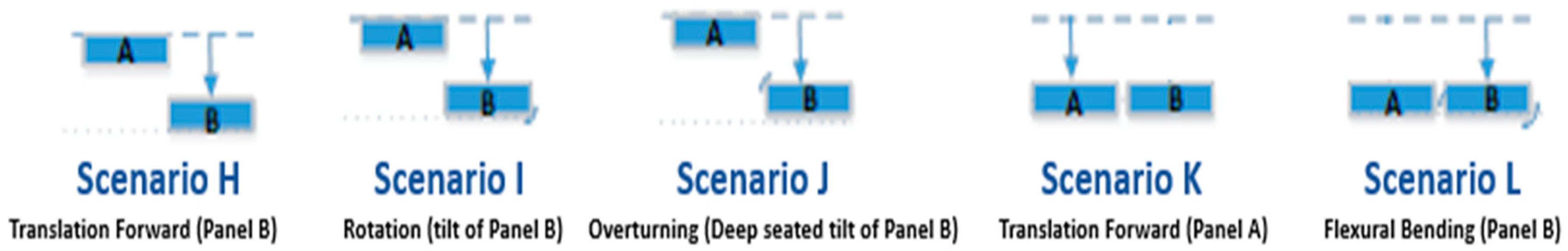
To deploy this photogrammetric approach, a novel observation of displacement and spatial changes along the surface of a retaining wall model was performed [9]. A 2.43 m × 2.43 m (8 ft × 8 ft) retaining wall model, consisting of two 1.22 m × 2.43 m (4ft × 8ft) panels, A and B, was subjected to four common displacement failure modes [39,40,41]. These failure modes were categorized into five testing scenarios: forward translation of wall panel B (scenario H), forward tilted rotation of wall panel B (scenario I), deep seated overturned rotation of wall panel B (scenario J), forward translation of wall panel A (scenario K) and flexural bending of wall panel B (scenario L) [9]. A brief schematic of the top of the retaining wall panels, providing a plan view for each of the five simulated failure scenarios, is shown in Figure 1. Fourteen reference control points were placed in the test setup to infer ground location for georeferencing. Ten of these control points were placed on the individual retaining wall panels, with five on each panel, and the remaining four were placed on neighboring stationary objects positioned at different elevations and depths from the wall model. The stationary control points, those placed on static surfaces, assisted in the co-registration of the point clouds in a common coordinate system for the different scenarios [9].
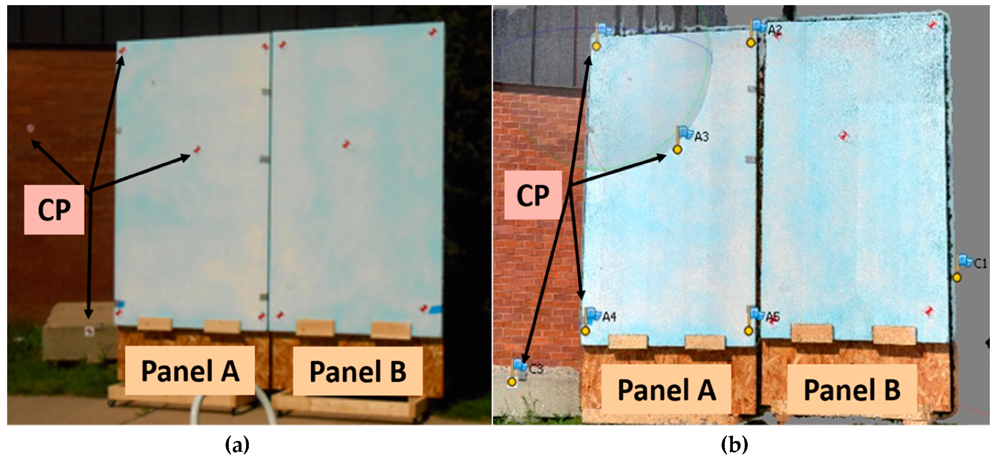
For each of the five scenarios, two images were collected, one kneeling and one standing, to produce vertical parallax from at least ten different positions from a 25-foot perpendicular line of sight [9]. A Nikon D5100 was used to collect images with a 55-mm focal length lens. At the end of each testing scenario configuration, a Trimble S3 Robotic total station (TS) surveying device, of 0.91 mm precision, was used to capture the location of the control points under failure simulation [9]. Figure 2a shows the setup of the wall model, with reference control points (CP) identified on the panels, as well as the static locations, such as the neighboring building wall and concrete platform. The photos taken from each scenario were placed into two commonly-used, commercially-available software packages, Agisoft Photoscan and Pix4D.
The software uses the control points to best align all images in the dataset. The photogrammetry point cloud models consist of numerous sets of points in 3D, on the order of several million. This magnitude of points results in point densities of tens– to hundreds–of–thousands of points per m2 [9]. Figure 2b provides an illustration of the point cloud model, including the flagged referenced control points within the testing environment. Control points on the moving wall panels were compared between scenarios, but also with total station measurements of those same points. The displacements were calculated by comparing the positions of the control points along the surfaces, for different scenarios. The relative space coordinate locations of the control points were determined in each of these scenarios, which were compared to the ground truth total station measurements.
A focused evaluation, considering different amounts of control points, was also performed for each of the five failure mode scenarios, specifically using the Photoscan software’s 3D model. Three sets of data, i.e., point cloud models, were created by aligning the collected images: (1) without any of the reference control points, (2) with two of the stationary control points and (3) with all four stationary control points. This strategy was implemented to consider the impact of control points for the model creation, varying from zero to four control points. For all three datasets, the locations of the wall panel control points, and two stationary points, were captured in the point cloud models and compared to the same total station measured locations. A rescaling adjustment factor was also included to present a best-fit evaluation, by knowing the distances of the control points and alignment of the points in space.
3. Results and Discussion
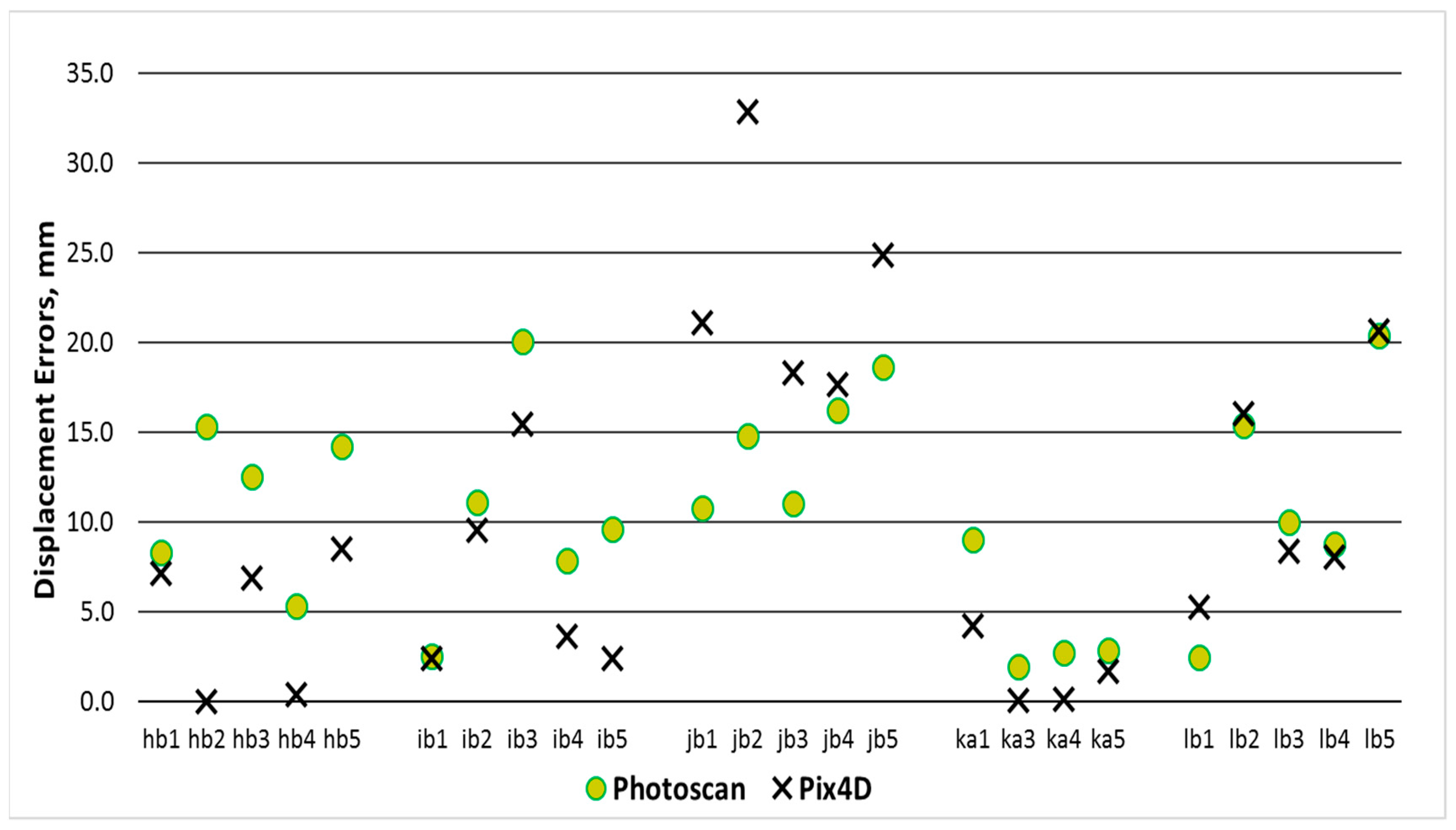
For each of the testing scenarios, the control point measurements captured from the photogrammetric models (shown in Figure 2b) were compared with the total station measurements, and corresponding differences or errors in the measurements were produced. Figure 3 reveals a comparison of the control point displacement errors for both the Photoscan and Pix4D software. The x-axis indicates the testing scenario evaluated and corresponding control points on the panel. Each of the scenarios are highlighted, along with the numbered control points (labeled from 1–5), along the particular panel’s A or B surface. The maximum displacement error is 35 mm with an average mean error of all control points determined as 10.5 mm for Photoscan and 9.8 mm for Pix4D (Figure 3). Scenario K presents the smallest errors (mean error of 4.1 mm and 1.5 mm, respectively, for Photoscan and Pix4D) across the five control point locations, when compared to the total station measurements. The largest errors are shown in scenario J, with a mean error of 14.3 mm and 23.9 mm, respectively, for Photoscan and Pix4D. On average, there is nearly a 10 mm difference between the two software programs within scenario J, which could be due to the complexity in modeling the imposed deep-seated failure on the wall within each software’s design.
Scenarios H, I and L experience unique translational, rotational and bending simulation, with average errors ranging between the largest (scenario J) to the smallest (scenario K). When comparing the displacement values captured with the total station, and those with the Pix4D software, percent errors are as small as 0.6% for control point location a4, in scenario K, and even smaller in scenario H, for control point b2 (less than 0.0049%). Percent errors with Photoscan were slightly larger, with the smallest, comparing the total station and software’s outputs, capturing a 3.4% error. These accuracy values are comparable with other researchers’ documenting accuracies, within an average range of 3.3–20.9 mm, when deploying traditional TLS techniques for infrastructure systems [42,43]. Digital Image Correlation (DIC) was implemented for measuring in situ deformation of the retaining wall, obtaining an accuracy of 3 mm, which further advocated for development of 3D model inclusion [44]. Several photogrammetric, unmanned aerial applications indicated 0.03–0.25 m range accuracy in assessing digital surface models [29], and accuracies near 4 cm with an aerial multi stereo approach [45].
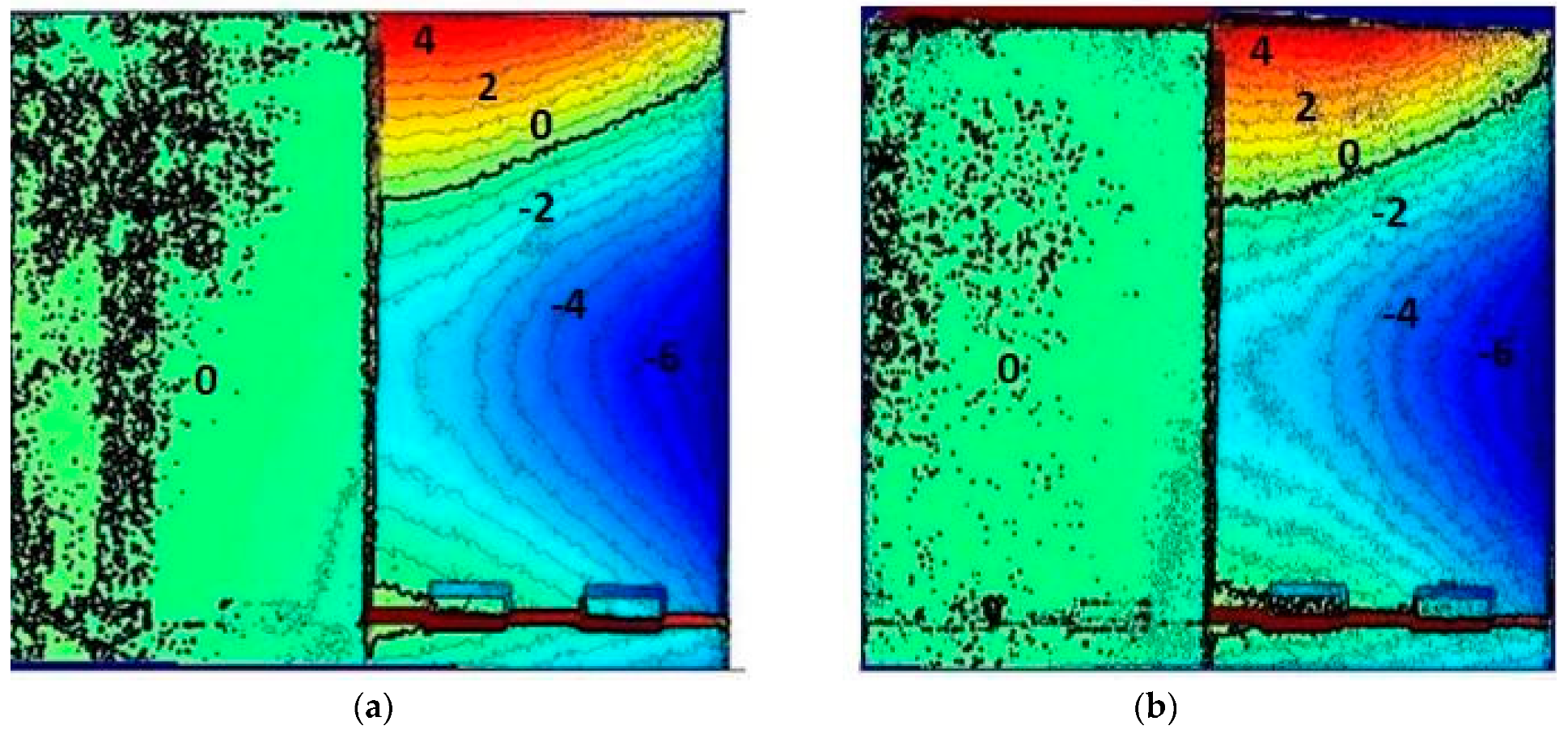
Further assessment of the data outputs was performed beyond the confined point locations with the wall’s displacement contour plots. Figure 4 reveals the plane-perpendicular displacement, shown as a color range with equal value contours, between the two software’s outputs for scenario L, the flexural bending failure model. The left panel remained stationary, and this is shown by the near-zero displacement. The right panel shows the simulated bending failure behavior displacements up to −6 cm (or 60 mm) for both Photoscan and Pix4D (Figure 4). The displacement contour along the surface plane shows little differences between the Photoscan (Figure 4a) and Pix4D (Figure 4b) software outputs. However, more detailed artifacts are visible along the Pix4D plane contour (Figure 4b), which is more evident on the right panel contour lines from imposed bending.
Distinctions in processing and modeling features, including noise rectifications between the two software programs, could have attributed to the variation in outputs. Nonetheless, this figure illustrates the feasibility of photogrammetric analysis for capturing changes along the surface of the infrastructure system, providing more descriptive data. This would enable a current, detailed performance or condition monitoring system, for infrastructure deformation, to effectively manage systems over a series of events (or time).
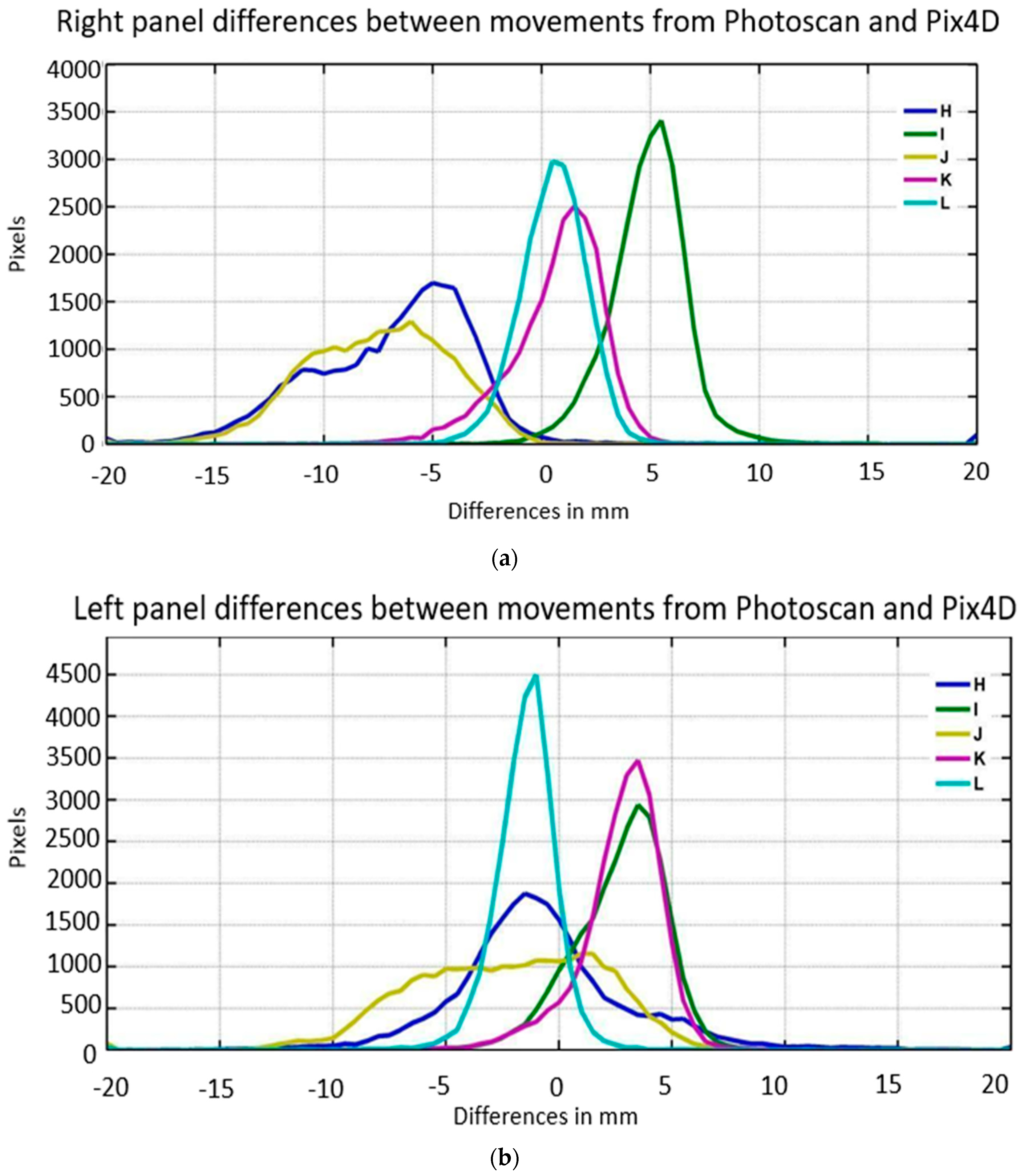
An analysis of the differences between the Photoscan and Pix4D results is presented in Figure 5 as a frequency polygon plot of the differences in the model outputs for the scenarios H through L. Scenario H and J present the widest distribution of differences (ranging from zero to slightly past −15 mm). In this regard, Figure 5a also aligns with the Figure 3 output, with the greatest discrepancy between the two software programs revealed in scenario H and J along the right panel or also referred as panel B. The other scenarios reveal a close-to-zero difference between the two software programs for the majority of the pixels on the model’s image. Overall, the agreement between the results from both software packages is high, and we can consider the differences to be less than 1 cm in general. Figure 5b presents similar results to those shown in Figure 5a, with results from both models generally falling within 1 cm of each other, revealing close values and high precision in change detection processes.
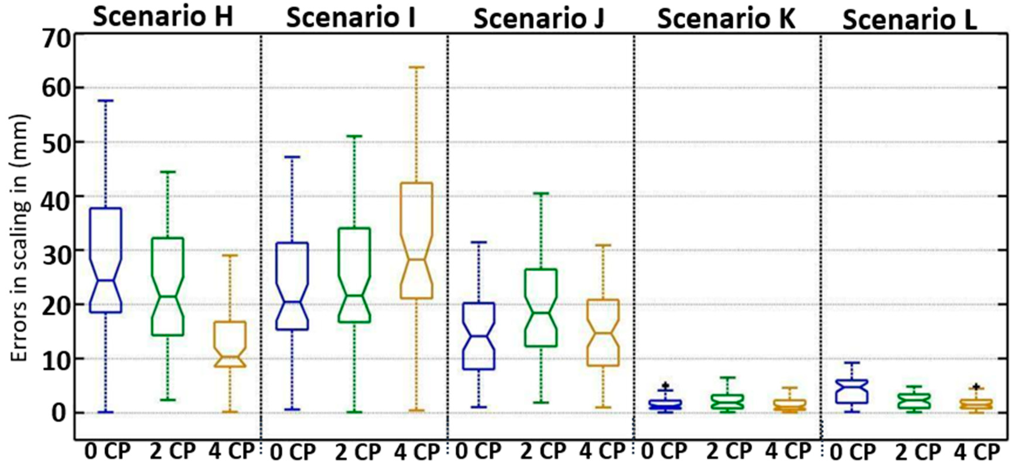
These results revealed comparable, and, even more accurate measures, when compared with other photogrammetric aerial investigations. Bakula et al. (2016), incorporating photogrammetry for measuring infrastructures as a part of unmanned aerial systems, obtained proven accuracies within 10 cm [46]. A greater optimal accuracy, near 5 cm, was captured when an iterative control point method was deployed [46]. Udin and Ahmad (2014) also presented submeter accuracies using UAV photogrammetry for large-scale stream mapping [36]. Additionally, the impact of choosing different configurations and numbers of control points was investigated for three different point cloud models using zero, two, and four control points for georeferencing. Figure 6 shows a comparison of the control point distributions when evaluated with the Photoscan software. Error ranges are significantly larger for scenarios H, I and J, than for the rest of the scenarios. The results shown in Figure 6 suggests that increasing the amount of control points does not, necessarily, lead to smaller errors. Therefore, a minimal implementation of control points, depending on the project, could be adequate for accurate 3D modeling.
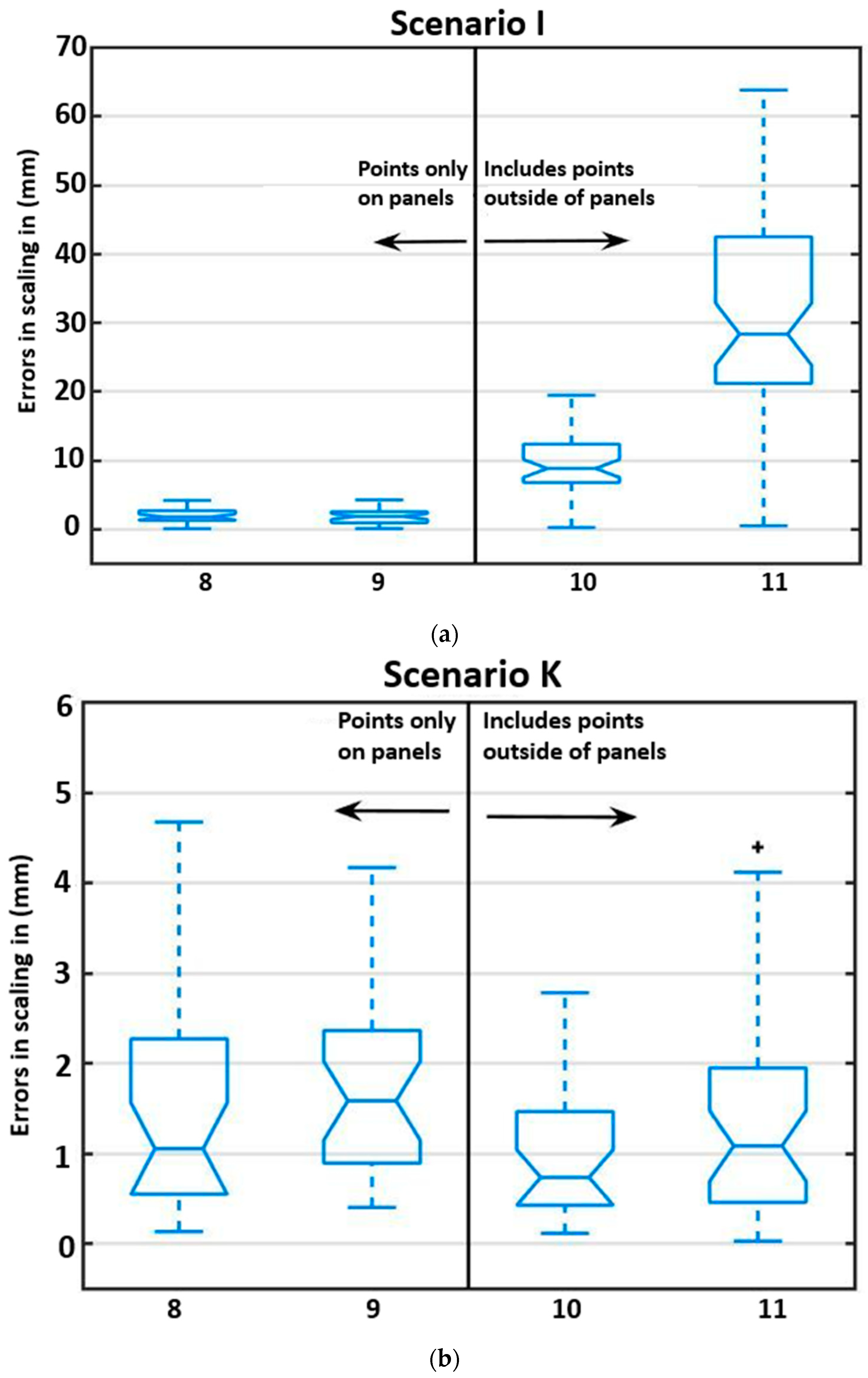
As the control points used in georeferencing increased from two to four, the spatial position of the points was also increased. This was shown to have a different impact in the scenarios H–J and scenarios K–L. Figure 7a. presents the results for scenario I, with the control points on the wall panels themselves and with the stationary control points. Scenario I presents a unique illustration in which the control point’s inclusion actually increased errors, particularly as they increased from two to four control points, unlike many of the other scenarios. In this scenario, as with others, the control points on each of the wall panels, and the four stationary points positioned on objects (two of which can be noted on the building wall and concrete platform in Figure 2b) near to the retaining wall model, at varying elevations, were used for referencing. The inclusion of the four control points produced larger errors.
This error, or change in results, may be related to the distribution of the additional control points incorporated in the analysis; the additional points were much farther away from the rest of the points and could, therefore, carry larger uncertainties, affecting the overall error values (Figure 6). When scenario I was evaluated using only the control points on the wall panels, A and B (and not the two stationary control points, as previously), a smaller error range was obtained (see left side of Figure 7a). The values along the x-axis in Figure 7. indicate the number of control points used, and a large increase in the error is observed when the number of control points used changes from 9 to 10. On the other hand, scenario K doesn’t show such an increase in the error with the different selection of control points (Figure 7b).
With distribution concerns, Gindraux et al. (2017) also assessed the accuracy of DSMs using UAV photogrammetry for glacier movement detection, in which the study emphasized accuracy decreases with closer distances to the GCP [29]. Liew et al. (2012) data highlighted that the center distribution of the control points presented the lowest total RMSE, lower than 5 pixels in aerial geometric distribution [35]. This may not, necessarily, be true, as our Figure 7b indicates reduction of error when control points beyond the center distribution were considered. Nonetheless, our results, and others overall, encourage uniformity in distributing control points.
To the contrary, when considering the amount of control points, researchers have presented varying findings. Shahbazi et al. (2015) suggests that, to reach the highest accuracy, a large number of well-distributed GCPs could be provided for a UAV-photogrammetry, DSM-georeferenced application of a gravel pit landscape, which may not, necessarily, be regarded as a minimum, but rather, a maximum amount [47]. Similarly, Tahar (2013), Rosnell and Hankavaara (2012) also promoted an increase in control points for improved DSM accuracy [33,48]. However, our study aligns with the notion of installing them at height variations, and even along different sides of the imaging zone, as Shahbazi documents, as well [46]. Gindraux et al. (2017), and other researchers, [49,50] also determined a common analysis, indicating accuracy increases with increased GCPs until a certain density is reached [29].
From this evaluation, a few considerations can be gathered. 3D modeling software is able to capture failure displacement, even with complex rotational movements with small errors. Test results from photogrammetry methods compared well with traditional measurements. The spatial distribution of control points may influence the quality of the results and could provide a considerable impact when detecting changes of an infrastructure system. Well-distributed control points are expected to produce better results, and minimal control points may enable an optimal density accuracy. Great precision between comparable modeling software further advocates the capability of photogrammetric processing for retaining wall performance monitoring.
The study also advocates the use of photogrammetry for, not only qualitative, but quantitative, data management of buildings and structures. Moreover, this study promotes the need for effective tools to manage risks and to ensure that performance-based requirements are met, as the research notes [13,26]. Maintaining performance data for transportation systems has been noted as a key element for transportation asset operation and planning [51], which photogrammetry methods could supplement and expand. The use of photogrammetry technologies for asset and, even, system-risk management, could be further considered to provide up-to-date measurements for a range of infrastructure corridors, whether transportation, civil or geotechnical. Additional investigation for obtaining accurate 3D models in photogrammetry software, considering testing setup or space configuration, anticipated displacement behavior, software specifications, camera settings, and increased or varied control point designs, should be pursued in future work.
4. Conclusions
Photogrammetry has the ability to generate 3D models of an object and enables a detailed description of changes in position or displacements over time. This study presents the evaluation of two widely-used photogrammetry software packages for capturing spatial and displacement changes of a retaining wall model. This study also shows the significance of the control points in evaluations and influences that may need to be considered for infrastructure monitoring. Implications of increasing control points for model reconstruction demonstrated that the inclusion of control points does not, necessarily, enhance model quality in georeferencing, but the position and distribution of the control points can influence model accuracy. It is recognized that spatial arrangement of control points needs considerable attention to adequately scale the 3D point cloud models and obtain optimal accuracy.
Author Contributions
R.C.O., R.E.-W. and T.O. conceived and designed the experiments; R.C.O., R.E.-W. and T.O. performed the experiments; R.C.O. and R.E.-W. analyzed the data; R.C.O., R.E.-W. and T.O. wrote the paper.
Funding
This research was partially funded by the U.S. Department of Transportation (USDOT) through the Office of the Assistant Secretary for Research and Technology (Cooperative Agreement No. RITARS-14-H-MTU).
Acknowledgments
This project was supported by several departments at Michigan Technological University including Geological and Mining Engineering and Sciences, Civil & Environmental Engineering, and School of Technology.
Conflicts of Interest
The authors declare no conflict of interest.
Disclaimer
The views, opinions, findings, and conclusions reflected in this paper are the responsibility of the authors only and do not represent the official policy or position of the USDOT/OST-R or any state or other entity.
References
- Wolf, P.R.; Dewitt, B.A.; Wilkinson, B.E. Elements of Photogrammetry: With Applications in GIS; McGraw-Hill: New York, NY, USA, 2000. [Google Scholar]
- Khaloo, A.; Lattanzi, D. Hierarchical dense structure-from-motion reconstructions for infrastructure condition assessment. J. Comput. Civ. Eng. 2016, 31, 04016047. [Google Scholar] [CrossRef]
- Han, J.; Hong, K.; Kim, S. Application of a photogrammetric system for monitoring civil engineering structures. In Special Applications of Photogrammetry; InTech: London, UK, 2012. [Google Scholar]
- Dai, F.; Rashidi, A.; Brilakis, I.; Vela, P. Comparison of image-based and time-of-flight-based technologies for three-dimensional reconstruction of infrastructure. J. Constr. Eng. Manag. 2012, 139, 69–79. [Google Scholar] [CrossRef]
- Dai, F.; Lu, M.; Kamat, V.R. Analytical approach to augmenting site photos with 3D graphics of underground infrastructure in construction engineering applications. J. Comput. Civ. Eng. 2010, 25, 66–74. [Google Scholar] [CrossRef]
- Zhu, Z.; Brilakis, I. Comparison of optical sensor-based spatial data collection techniques for civil infrastructure modeling. J. Comput. Civ. Eng. 2009, 23, 170–177. [Google Scholar] [CrossRef]
- Kim, D.H.; Gratchev, I.; Balasubramaniam, A. A photogrammetric approach for stability analysis of weathered rock slopes. Geotech. Geol. Eng. 2015, 33, 443–454. [Google Scholar] [CrossRef]
- Ceylan, H.; Gopalakrishnan, K.; Kim, S.; Taylor, P.C.; Prokudin, M.; Buss, A.F. Highway infrastructure health monitoring using micro-electromechanical sensors and systems (MEMS). J. Civ. Eng. Manag. 2013, 19, S188–S201. [Google Scholar] [CrossRef]
- Oats, R.C.; Escobar-Wolf, R.; Oommen, T. A Novel Application of Photogrammetry for Retaining Wall Assessment. Infrastructures 2017, 2, 10. [Google Scholar] [CrossRef]
- Anderson, S.A.; Alzamora, D.; DeMarco, M.J. Asset Management Systems for Retaining Wall. In Proceedings of the Biennial Geotechnical Seminar Conference, Denver, CO, USA, 7 November 2008; pp. 162–177. [Google Scholar]
- Butler, C.J.; Gabr, M.A.; Rasdorf, W.; Findley, D.J.; Chang, J.C.; Hammit, B.E. Retaining wall field condition inspection, rating analysis, and condition assessment. J. Perform. Constr. Facil. 2015, 30, 04015039. [Google Scholar] [CrossRef]
- AASHTO. Transportation Asset Management Guide: A Focus on Implementation; American Association of State Highway and Transportation Officials (AASHTO): Washington, DC, USA, 2013. [Google Scholar]
- Almeida, N.M.; Sousa, V.; Dias, L.A.; Branco, F. Engineering risk management in performance-based building environments. J. Civ. Eng. Manag. 2015, 21, 218–230. [Google Scholar] [CrossRef]
- Bhatla, A.; Choe, S.Y.; Fierro, O.; Leite, F. Evaluation of accuracy of as-built 3D modeling from photos taken by handheld digital cameras. Autom. Constr. 2012, 28, 116–127. [Google Scholar] [CrossRef]
- Riveiro, B.; Jauregui, D.V.; Arias, P.; Armesto, J.; Jiang, R. An innovative method for remote measurement of minimum vertical underclearance in routine bridge inspection. Autom. Constr. 2012, 25, 34–40. [Google Scholar] [CrossRef]
- Golparvar-Fard, M.; Bohn, J.; Teizer, J.; Savarese, S.; Peña-Mora, F. Evaluation of image-based modeling and laser scanning accuracy for emerging automated performance monitoring techniques. Autom. Constr. 2011, 20, 1143–1155. [Google Scholar] [CrossRef]
- Zhou, Z.; Gong, J.; Guo, M. Image-based 3D reconstruction for post-hurricane residential building damage assessment. J. Comput. Civ. Eng. 2015, 30, 04015015. [Google Scholar] [CrossRef]
- Clayton, C.R.; Woods, R.I.; Bond, A.J.; Milititsky, J. Earth Pressure and Earth-Retaining Structures; CRC Press: Boca Raton, FL, USA, 2014. [Google Scholar]
- DeMarco, M.J.; Anderson, S.A.; Armstrong, A. Retaining Walls Are Assets Too! Public Roads 2009, 73, 30–37. [Google Scholar]
- Gul, M.; Catbas, F.N.; Hattori, H. Image-based monitoring of open gears of movable bridges for condition assessment and maintenance decision making. J. Comput. Civ. Eng. 2013, 29, 04014034. [Google Scholar] [CrossRef]
- Slaker, B.A. Monitoring Underground Mine Displacement Using Photogrammetry and Laser Scanning. Ph.D. Thesis, Virginia Polytechnic Institute and State University, Blacksburg, VA, USA, 2015. [Google Scholar]
- Escobar-Wolf, R.; Oommen, T.; Brooks, C.N.; Dobson, R.J.; Ahlborn, T.M. Unmanned aerial vehicle (UAV)-based assessment of concrete bridge deck delamination using thermal and visible camera sensors: A preliminary analysis. Res. Nondestruct. Eval. 2018, 29, 183–198. [Google Scholar] [CrossRef]
- Kalacska, M.; Lucanus, O.; Sousa, L.; Vieira, T.; Arroyo-Mora, J.P. UAV-Based 3D Point Clouds of Freshwater Fish Habitats, Xingu River Basin, Brazil. Data 2019, 4, 9. [Google Scholar] [CrossRef]
- Scotland, I.; Dixon, N.; Frost, M.W.; Wackrow, R.; Fowmes, G.J.; Horgan, G. Measuring Deformation Performance of Geogrid Reinforced Structures Using a Terrestrial Laser Scanner; Loughborough University Institutional Repository: Leicestershire, UK, 2014. [Google Scholar]
- Mill, T.; Alt, A.; Liias, R. Combined 3D building surveying techniques–terrestrial laser scanning (TLS) and total station surveying for BIM data management purposes. J. Civ. Eng. Manag. 2013, 19, S23–S32. [Google Scholar] [CrossRef]
- Henke, K.; Pawlowski, R.; Schregle, P.; Winter, S. Use of digital image processing in the monitoring of deformations in building structures. J. Civ. Struct. Health Monit. 2015, 5, 141–152. [Google Scholar] [CrossRef]
- Jiang, R.; Jáuregui, D.V.; White, K.R. Close-range photogrammetry applications in bridge measurement: Literature review. Measurement 2008, 41, 823–834. [Google Scholar] [CrossRef]
- Calì, M.; Ambu, R. Advanced 3D Photogrammetric Surface Reconstruction of Extensive Objects by UAV Camera Image Acquisition. Sensors 2018, 18, 2815. [Google Scholar] [CrossRef]
- Gindraux, S.; Boesch, R.; Farinotti, D. Accuracy assessment of digital surface models from unmanned aerial vehicles’ imagery on glaciers. Remote Sens. 2017, 9, 186. [Google Scholar] [CrossRef]
- Westoby, M.J.; Brasington, J.; Glasser, N.F.; Hambrey, M.J.; Reynolds, J.M. Structure-from-Motion’ photogrammetry: A low-cost, effective tool for geoscience applications. Geomorphology 2012, 179, 300–314. [Google Scholar] [CrossRef]
- Forlani, G.; Pinto, L.; Roncella, R.; Pagliari, D. Terrestrial photogrammetry without ground control points. Earth Sci. Inform. 2014, 7, 71–81. [Google Scholar] [CrossRef]
- Dai, F.; Feng, Y.; Hough, R. Photogrammetric error sources and impacts on modeling and surveying in construction engineering applications. Visual. Eng. 2014, 2, 2. [Google Scholar] [CrossRef] [Green Version]
- Tahar, K.N. An evaluation on different number of ground control points in unmanned aerial vehicle photogrammetric block. Int. Arch. Photogramm. Remote Sens. Spat. Inf. Sci. 2013, 40, 93–98. [Google Scholar] [CrossRef]
- Benassi, F.; Dall’Asta, E.; Diotri, F.; Forlani, G.; Morra di Cella, U.; Roncella, R.; Santise, M. Testing accuracy and repeatability of UAV blocks oriented with GNSS-supported aerial triangulation. Remote Sens. 2017, 9, 172. [Google Scholar] [CrossRef]
- Liew, L.H.; Wang, Y.C.; Cheah, W.S. Evaluation of control points’ distribution on distortions and geometric transformations for aerial images rectification. Procedia Eng. 2012, 41, 1002–1008. [Google Scholar] [CrossRef]
- Udin, W.S.; Ahmad, A. Assessment of photogrammetric mapping accuracy based on variation flying altitude using unmanned aerial vehicle. In IOP Conference Series: Earth and Environmental Science; IOP Publishing: Bristol, UK, 2014; Volume 18, p. 012027. [Google Scholar]
- Chen, Y.C.; Tseng, Y.H. Advancement of Close Range Photogrammetry with a Portable Panoramic Image Mapping System (Ppims); The Photogrammetric Record: Hoboken, NJ, USA, 2018. [Google Scholar]
- Fraser, C. Advances in Close Range Photogrammetry. Available online: www.ifp.uni-stuttgart.de/publications/phowo15/260Fraser.pdf (accessed on 25 September 2018).
- Federal Highway Administration United States Department of Transportation. Mechanically Stabilized Earth Walls and Reinforced Soil Slopes Design & Construction Guidelines; Publication No. FHWA-NHI-00-043; National Highway Institute (NHI) Office of Bridge Technology: Washington, DC, USA, 2001.
- Power, M.; Fishman, K.L.; Makdisi, F.; Musser, S.; Richards, R., Jr.; Youd, T.L. Seismic Retrofitting Manual for Highway Structures: Part 2-Retaining Structures, Slopes, Tunnels, Culverts and Roadways; Federal Highway Administration: Washington, DC, USA, 2006.
- Muni, B. Soil Mechanics & Foundations; John Wiley & Sons, Inc.: Hoboken, NJ, USA, 2010. [Google Scholar]
- Su, Y.Y.; Hashash, Y.M.A.; Liu, L.Y. Integration of construction as-built data via laser scanning with geotechnical monitoring of urban excavation. J. Constr. Eng. Manag. 2006, 132, 1234–1241. [Google Scholar] [CrossRef]
- Gong, J.; Zhou, H.; Gordon, C.; Jalayer, M. Mobile terrestrial laser scanning for highway inventory data collection. Comput. Civ. Eng. 2012, 545–552. [Google Scholar] [CrossRef]
- Tung, S.H.; Weng, M.C.; Shih, M.H. Measuring the in situ deformation of retaining walls by the digital image correlation method. Eng. Geol. 2013, 166, 116–126. [Google Scholar] [CrossRef]
- Maltezos, E.; Skitsas, M.; Charalambous, E.; Koutras, N.; Bliziotis, D.; Themistocleous, K. Critical infrastructure monitoring using UAV imagery. In Fourth International Conference on Remote Sensing and Geoinformation of the Environment (RSCy2016); International Society for Optics and Photonics: Bellingham, WA, USA, 2016; Volume 9688, p. 96880P. [Google Scholar]
- Bakula, K.; Ostrowski, W.; Szender, M.; Plutecki, W.; Salach, A.; Górski, K. Possibilities for Using LIDAR and Photogrammetric Data Obtained with AN Unmanned Aerial Vehicle for Levee Monitoring. Int. Arch. Photogramm. Remote Sens. Spat. Inf. Sci. 2016, 41, 773–780. [Google Scholar] [CrossRef]
- Shahbazi, M.; Sohn, G.; Théau, J.; Menard, P. Development and evaluation of a UAV-photogrammetry system for precise 3D environmental modeling. Sensors 2015, 15, 27493–27524. [Google Scholar] [CrossRef]
- Rosnell, T.; Honkavaara, E. Point cloud generation from aerial image data acquired by a quadrocopter type micro unmanned aerial vehicle and a digital still camera. Sensors 2012, 12, 453–480. [Google Scholar] [CrossRef]
- Rock, G.; Ries, J.B.; Udelhoven, T. Sensitivity analysis of UAV-photogrammetry for creating digital elevation models (DEM). Int. Arch. Photogramm. Remote Sens. Spat. Inf. Sci. 2011, XXXVIII-1/C22, 69–73. [Google Scholar] [CrossRef]
- Tonkin, T.N.; Midgley, N.G. Ground-control networks for image based surface reconstruction: An investigation of optimum survey designs using UAV derived imagery and structure-from-motion photogrammetry. Remote Sens. 2016, 8, 786. [Google Scholar] [CrossRef]
- Sisiopiku, V.P.; Rostami-Hosuri, S. Congestion Quantification Using the National Performance Management Research Data Set. Data 2017, 2, 39. [Google Scholar] [CrossRef]
Figure 1.
Plan view illustration of the simulated failure mode scenarios and movement for each wall panel.
Figure 1.
Plan view illustration of the simulated failure mode scenarios and movement for each wall panel.

Figure 2.
Images of retaining wall model (a) during data collection and (b) point cloud reconstructed model with flagged control points.
Figure 2.
Images of retaining wall model (a) during data collection and (b) point cloud reconstructed model with flagged control points.

Figure 3.
Displacement errors captured with Photoscan and Pix4D.

Figure 4.
Photogrammetry plane-perpendicular displacement for scenarios L using (a) Photoscan and (b) Pix4D software programs (in cm).
Figure 4.
Photogrammetry plane-perpendicular displacement for scenarios L using (a) Photoscan and (b) Pix4D software programs (in cm).

Figure 5.
Histogram of errors between softwares for all scenarios H-L for both the (a) left panel (panel-A) and (b) right panel (panel-B).
Figure 5.
Histogram of errors between softwares for all scenarios H-L for both the (a) left panel (panel-A) and (b) right panel (panel-B).

Figure 6.
Errors in control point evaluation for scenarios H–L.

Figure 7.
Comparison of error analysis for spatial variation of control points in (a) scenario I and (b) scenario K.
Figure 7.
Comparison of error analysis for spatial variation of control points in (a) scenario I and (b) scenario K.

© 2019 by the authors. Licensee MDPI, Basel, Switzerland. This article is an open access article distributed under the terms and conditions of the Creative Commons Attribution (CC BY) license (http://creativecommons.org/licenses/by/4.0/).
Share and Cite
MDPI and ACS Style
Oats, R.C.; Escobar-Wolf, R.; Oommen, T. Evaluation of Photogrammetry and Inclusion of Control Points: Significance for Infrastructure Monitoring. Data 2019, 4, 42. https://0-doi-org.brum.beds.ac.uk/10.3390/data4010042
AMA Style
Oats RC, Escobar-Wolf R, Oommen T. Evaluation of Photogrammetry and Inclusion of Control Points: Significance for Infrastructure Monitoring. Data. 2019; 4(1):42. https://0-doi-org.brum.beds.ac.uk/10.3390/data4010042
Chicago/Turabian StyleOats, Renee C., Rudiger Escobar-Wolf, and Thomas Oommen. 2019. "Evaluation of Photogrammetry and Inclusion of Control Points: Significance for Infrastructure Monitoring" Data 4, no. 1: 42. https://0-doi-org.brum.beds.ac.uk/10.3390/data4010042