Towards Sentinel-1 SAR Analysis-Ready Data: A Best Practices Assessment on Preparing Backscatter Data for the Cube

Abstract

This study aims at assessing the feasibility of automatically producing analysis-ready radiometrically terrain-corrected (RTC) Synthetic Aperture Radar (SAR) gamma nought backscatter data for ingestion into a data cube for use in a large spatio-temporal data environment. As such, this study investigates the analysis readiness of different openly available digital elevation models (DEMs) and the capability of the software solutions SNAP and GAMMA in terms of overall usability as well as backscatter data quality. To achieve this, the study builds on the Python library pyroSAR for providing the workflow implementation test bed and provides a Jupyter notebook for transparency and future reproducibility of performed analyses. Two test sites were selected, over the Alps and Fiji, to be able to assess regional differences and support the establishment of the Swiss and Common Sensing Open Data cubes respectively.

1. Introduction

Global Earth systems are facing increased pressure—over-exploitation of resources, climate change, environmental and ecological degradation, and overpopulation—meaning that the ability to measure and monitor Earth surface change is of ever-increasing value [1]. Advances in technology, the democratization of space and recognition of the value of Earth Observation (EO) in providing insights—e.g., for the Sustainable Development Agenda—have led to an increase in the availability of EO data worldwide, and with this, a growing interest globally in efficient exploitation of EO data at scale [2]. Global monitoring programs coupled with an extensive archive of historical remotely sensed imagery have paved the way for both historic time-series analysis and operational routine monitoring [3].

The launch of the set of Sentinel satellites by the European Space Agency (ESA) as part of the European Commission’s Copernicus Program has been a catalyst for this change and is generating ever-increasing interest across governments and different market sectors, each with different user requirements [4]. It becomes quickly apparent that it is simply not technically feasible or financially affordable to consider traditional methods of storing, handling and manipulating EO data. Local processing and data distribution methods currently exploited by industry and government are not suitable to address the challenge of scalability, increases in the size of data volumes, and the growing complexities in the preparation, handling, storage, and analysis required to meet user requirements. To allow immediate analysis of the data without additional significant user effort, these barriers need to be addressed. In response, there has been a drive within the EO community to find faster, cost-effective ways to process EO data at scale, whilst facilitating access to EO-derived insights. Two concepts addressing this challenge are Earth Observation Data Cubes (EODC), coupled with the concept of Analysis-Ready Data (ARD) [5,6].

As a geodata infrastructure technology for convenient storage and analysis of large amounts of raster data, the concept of data cubes has been gaining ground. In particular, the Open Data Cube (ODC), originally developed by Geoscience Australia (GA) and having evolved as an international initiative supported by the Committee of Earth Observation Satellites (CEOS), has found wide application in part due to its user-friendly Python application programming interface (API). Several efforts from CEOS and national ODC initiatives, such as the Swiss Data Cube (SDC) [7], the Common Sensing Data Cube (CSDC), the Ghana Data Cube [8], and Digital Earth Australia (DEA) [9] are working towards making EO data accessible and are discussing which data specifications need to be met to optimally provide data over this new infrastructure.

Synthetic Aperture Radar (SAR) is an EO system that has the advantage of being almost weather and solar illumination independent. Therefore, SAR data, and more specifically, Sentinel-1 is becoming popular, as many regions have issues with cloud cover, and would benefit from denser temporal sampling, e.g. for applications such as forest change detection and coastal monitoring. Through the Copernicus program, Sentinel-1 data is routinely and freely available. With the availability of ESA’s Sentinels Application Platform (SNAP) open-source software, the access barrier to SAR data has been significantly lowered. Large amounts of SAR data acquired with a repeat interval of twelve days (reduced to six using both Sentinel-1A and Sentinel-1B) can be freely downloaded and conveniently processed [10,11].

However, to access the valuable information contained within EO data, users are required to undertake a series of complex pre-processing steps to turn the data from a ‘raw’ unprocessed format into a state that can be analyzed. Unless the user has the expertise, software and infrastructure to handle and process this information, efficient exploitation of the data is not realized.

A term that is now frequently used in this context is Analysis-Ready Data (ARD). According to the Committee on Earth Observation Satellites (CEOS), this is defined as ‘satellite data that have been processed to a minimum set of requirements and organized into a form that allows immediate analysis without additional user effort and interoperability with other datasets both through time and space’ (http://ceos.org/ard/).

Originally defined for optical satellite imagery, this generally describes data that is corrected for atmospheric effects and thus contains measurements of surface reflectance. Currently, the majority of known Data Cube implementations rely on optical imagery [9,12,13] and only a few of them offer access to SAR ARD products. One example of the use of SAR data in a Data Cube framework is the Water Across Synthetic Aperture Radar Data (WASARD) for water body classification [14]. Having SAR data in an Earth Observation Data Cube (EODC) can be an excellent complement to optical imagery and can overcome limitations such as cloud coverage. The main reason that there is currently little SAR data available in EODCs comes from the fact that there was, until recently, no common definition of the ARD level. CEOS is leading an effort to define the minimum set of requirements to allow immediate analysis with minimum additional user effort. The CEOS Analysis-Ready Data for Land (CARD4L—http://ceos.org/ard/) provides specifications for Optical, Thermal, and SAR imagery. Regarding SAR, the ARD level was recently defined only for terrain-corrected radar backscatter. Polarimetric and interferometric specifications are under development and are expected for 2019. CARD4L SAR products will be: (1) Normalized Radar Backscatter; (2) Geocoded Single-Look Complex; (3) Polarimetric Radar Decomposition; (4) Normalized Radar Covariance Matrix, and (5) Differential Interferometry Products [15]. To be considered as ARD, the Normalized Radar Backscatter product should be Radiometric Terrain Correction (RTC) and provided as gamma0 (γ0) backscatter, which mitigates systematic contamination that would otherwise still be present in sets of data acquired with multiple geometries [16].

While there is little dispute over the individual processing steps necessary to convert the original level 1 backscatter products provided by, e.g., Copernicus to RTC [16], different software implementations may lead to significant differences in final product quality. The Committee on Earth Observation Satellites (CEOS) recently published a comprehensive guide on how to produce Analysis-Ready SAR RTC data for land mapping applications, listing a large number of requirements for metadata specifications and necessary corrections to obtain a well-documented data set of high quality [15]. However, what remains missing, is a straightforward implementation in commercial and open-source software such that a user can directly select a certain level of quality and “analysis readiness”. Once the data is prepared to the highest standard possible, the influence of SAR-specific imaging effects is to be assessed. Effects such as geometric decorrelation are inherent to SAR data and while they are relevant to some applications, they can be considered as disturbances for others. Therefore, the user needs to be aware of them when analyzing any specific backscatter ARD product.

The overall aim of this study is to evaluate how far Sentinel-1 data is interoperable in terms of geometry and software. It picks up on findings reported in [17], however, investigating two new test areas; in the Alps and in Fiji. These test areas were selected as there is currently work underway on developing operational data cubes for these two areas (SDC—http://www.swissdatacube.ch, CSDC—http://commonsensing.org.gridhosted.co.uk/).

The SDC is an innovative analytical cloud-computing platform allowing users to access, analysis and visualization of 35 years of optical (e.g., Sentinel-2; Landsat 5, 7, 8) and radar (e.g., Sentinel-1) satellite EO ARD over the entire country [5,18]. Importantly, the SDC minimizes the time and scientific knowledge required for national-scale analyses of large volumes of consistently calibrated and spatially aligned satellite observations. The SDC is based on the Open Data Cube software stack [19,20] and is updated continually. It contains approximately 10,000 scenes for a total volume of 6TB and more than 200 billion observations over the Alps. The objective of the SDC is to support the Swiss government for environmental monitoring and reporting, as well as enabling Swiss scientific institutions to benefit from EO data for research and innovation. Additionally, the SDC allows for medium/high spatial and temporal resolution environmental monitoring, thereby providing synoptic, consistent and spatially explicit information sufficiently detailed to capture anthropogenic impacts at the national scale. The SDC is supported by the Swiss Federal Office for the Environment (FOEN) and currently is being developed, implemented and operated by the United Environment Program (UNEP)/GRID-Geneva in partnership with the University of Geneva (UNIGE), the University of Zurich (UZH) and the Swiss Federal Institute for Forest, Snow and Landscape Research (WSL). Ultimately, the SDC will deliver a unique capability to track changes in unprecedented detail using EO satellite data and enable more effective responses to problems of national significance [18]. To our knowledge, the Swiss Data Cube is the first Data Cube to contain almost the entire Sentinel-1 ARD archive. It contains five years of 12-day terrain-flattened backscatter Sentinel-1 backscatter composites generated using the methodology described in [16] in the initial stage.

For the SDC, Sentinel-1 data will be useful to enhance the Snow Observations from Space (SOfS) algorithm that currently only uses optical imagery (e.g., Landsat, Sentinel-2) [20]. Preliminary results have shown a clear decrease in snow cover over the Alps in the last 30 years. However, to provide an integrated and effective mechanism to monitor snow cover and its variability, SAR data will help identify snowmelt processes [21]. In addition to snow mapping, Sentinel-1 analysis-ready data has been shown to be useful for vegetation mapping and dynamics [22], rapid assessment after a storm event [23], and melt-onset mapping using multiple SAR sensors [24].

The Common Sensing project is an international development project that aims to improve climate change and disaster risk resilience in the Small-Island Developing States (SIDS) of Fiji, Vanuatu and the Solomon Islands (http://commonsensing.org.gridhosted.co.uk/) with the support of EO data and tools. As part of this multi-year project, an EODC for Fiji is being developed on the Open Data Cube software stack [19,20] and will contain Analysis-Ready Data for Sentinel-2, Landsat-5-8, SPOT 1-5 (surface reflectance) and Sentinel-1 (normalized radar backscatter). Much like the SDC, the Common Sensing Data Cube (CSDC) will be built with an aim to break down barriers to the use of EO data by policymakers through the provision of data and tools to facilitate rapid generation of EO-derived products and insights through both time and space. The objective is to support government and non-government stakeholders to undertake routine monitoring and reporting on Earth surface dynamics in rapidly changing environments in the South Pacific SIDS. For example, the CSDC will focus on exploitation of S1 data for vegetation mapping, coastal erosion, water resource management and disaster response, e.g., flooding.

As part of this study, different existing pre-processing workflows from different software solutions were evaluated for their interoperability. For instance, changes in backscatter from these differences might be too severe for certain mapping applications. Therefore, this study aimed at investigating the signal stability over different land cover classes to observe whether temporal backscatter variability originates from actual changes over land or are in fact the result of, e.g., different viewing angles or acquisition times. Of further interest in this context is a thorough analysis of how far the quality of the Digital Elevation Model (DEM) used in the processing affects the quality of the resulting products. Finally, this study provides an open-source assessment framework via a Python package including a Jupyter notebook (see Supplementary Materials).

Although compatibility with the CEOS ARD backscatter standard is, ultimately, to be reached, this study does not perform a formal assessment of the extent to which the specific requirements are met.

2. Study Outline and Description of Test Sites

This study investigated the use of two SAR processing software solutions, SNAP and GAMMA, for producing radiometrically terrain-corrected Sentinel-1 SAR backscatter. In particular, the influence of the resampling method and the DEM on the resulting topographic normalization was assessed. This section guides the reader through the paper’s structure. First, Chapter 3 describes the technical methodology of the study. In Chapter 4, the results from the analyses performed are presented. Chapters 5 and 6 discuss the findings and conclude. Motivated by the activities around the Swiss and Common Sensing Data Cubes, two test sites were selected, in the Alps and in Fiji, respectively.

In a first major component, two single S1A ground-range detected (GRD) scenes, acquired over the two test sites, were processed using two software solutions with different parametrizations and DEMs to assess the quality of the resulting RTC backscatter. This is described in Section 4.1, Section 4.2 and Section 4.3. The identifiers of the two scenes are presented in

Table 1. Identifiers of the scenes used for single image analysis.

Test Site	Scene Identifier
Alps	S1A_IW_GRDH_1SDV_20180829T170656_20180829T170721_023464_028DE0_F7BD
Fiji	S1A_IW_GRDH_1SDV_20181229T064000_20181229T064036_025236_02CA47_4B57

; their footprints are shown in Figure 1 and Figure 2. The footprints shown in these plots were used throughout the three mentioned sections to create DEMs of the same size and used the same inputs for the SAR processing.

These scenes were processed with the steps described in Section 3.3 to UTM Zone 32N (EPSG 32632) and Zone 60S (EPSG 32760), respectively, with a spatial resolution of 90 m. This resolution was chosen as a common denominator of all DEMs used in order to more objectively compare their quality independent of the differences in spatial resolution.

After thorough analysis of single image processing results, focus shifted to time series analysis in Section 4.4. For this, the study area was scaled down slightly to the island of Viti Levu, which can also be seen in Figure 2. Viti Levu is the largest island in the Fijian archipelago and the most populated. Sentinel-1 data is being routinely collected over Viti Levu from ascending and descending tracks every ~6 days; however, data is currently only being collected by Sentinel-1A. For this study, 62 Sentinel-1 GRD scenes acquired between April 2018 and April 2019 were processed in accordance with steps described in Section 3.3 and re-projected onto a UTM Zone 60S (EPSG 32760) grid with a sample interval of 20 m. An overview of Fiji, the study area for time series analysis, and the relevant S1 acquisition frames are displayed in Figure 3.

3. Methods

3.1. Software

This study and the accompanying Jupyter notebook (see Supplementary Materials) build on two Python packages pyroSAR [25,26] and spatialist [27]. PyroSAR is a framework for organizing and processing SAR data with APIs to the ESA Sentinel Application Platform (SNAP) [28] and GAMMA [29]. It serves the purpose of wrapping the image processing into convenient Python functions so that processing in SNAP and GAMMA can be operated in a similar way. Spatialist offers general spatial data handling functionality for pyroSAR by providing a convenient wrapper for the Python bindings of the Geodata Abstraction Library (GDAL) [30], offering a collection of general spatial data handling tools.

Several additions have been made to pyroSAR during this study, which are reflected in versions 0.7 to 0.9.1. A changelog summarizing these changes is available in pyroSAR’s online documentation [26].

While the workflows used during this study for processing with GAMMA and SNAP already existed, several additions and modifications were made to further improve the accuracy of the processing result and the usability of the routines within a Jupyter notebook.

Throughout this study, images were processed using SNAP version 6.0.9 and a GAMMA version released in November 2018. SNAP7 is due to be released in Summer 2019 with announced improvements to the terrain flattening procedure [31]. This processing step is particularly important for creating RTC products and processing results will be considered as soon as this new version is released to update the findings accordingly.

During this study, it was observed that SNAP processing of large workflows, i.e., with many processing steps in sequence, takes disproportionately longer, the more processing steps are added to it. For this reason, a mechanism was added to pyroSAR which splits a workflow into several groups, writes each group to a new temporary workflow XML file and executes these new workflows in sequence. Temporary products are written by the intermediate workflows, which are then passed to the succeeding workflow. Once finished, the directory containing the temporary workflows and products is deleted. This was observed to drastically increase processing speed, but no dedicated benchmarking was performed.

In addition to the Jupyter notebook technology [32], this study further builds on several open-source Python packages, in particular, Numpy [33] for general array handling, Matplotlib [34] for visualization, Scipy [35] and Astropy [36] for specific array computations and Scikit-Learn [37] for computation of performance statistics.

3.2. DEM Preparation

The choice of a high-quality DEM is crucial for accurate SAR processing, in particular for the correction of topographic effects such as foreshortening. According to the CEOS recommendations on producing analysis ready normalized backscatter for land [15], the selected DEM optimally has a spatial resolution as good or better than the resolution of the SAR image. Furthermore, it is recommended to assess whether the topography had changed between the acquisition of the DEM and that of the SAR scene to ensure that changes in backscatter are not related to changes in topography.

Thus, in this study, different DEMs were compared in order to assess the extent to which newer options are better suited for processing SAR imagery than older ones. Although newer DEMs might be closer in acquisition date to the SAR scene, older options have likely undergone more processor updates and manual edits to correct processor shortcomings over the years and might still be the better choice. See, e.g., [38] and [39] for details on SRTM quality enhancement.

The SAR processing was performed with four different DEMs, SRTM in 1 arcsec and 3 arcsec resolution [40], the 30 m ALOS World DEM (AW3D30) [41] and the TanDEM-X DEM in 90 m resolution [42]. An overview of DEM download URLs is given in

Table 2. Digital Elevation Models (DEMs) used in this study and their sources.

DEM	Source
ALOS World 3D 30 m	ftp://ftp.eorc.jaxa.jp/pub/ALOS/ext1/AW3D30/release_v1804
SRTM 1 arcsec	https://step.esa.int/auxdata/dem/SRTMGL1
SRTM 3 arcsec	http://srtm.csi.cgiar.org/wp-content/uploads/files/srtm_5x5/TIFF
TanDEM-X 90 m	ftpes://tandemx-90m.dlr.de

. For this study, routines were developed in pyroSAR to automatically prepare these different DEM types for processing in both SNAP and GAMMA software. This includes downloads of respective DEM tiles for a defined geometry, e.g., the footprint of a SAR scene, mosaicking and cropping, as well as re-projection and conversion from EGM96 geoid heights to WGS84 ellipsoid heights if necessary. Adopting this methodology, it was guaranteed that all DEM mosaics were created in an identical way—thereby mitigating inconsistencies introduced by the DEM preparation itself. The DEM files used for SNAP and GAMMA were thus identical aside from the file format, which was GeoTIFF for SNAP and the GAMMA file format in the latter.

To fully evaluate the quality of the respective DEMs, a high-resolution reference DEM, e.g., from a LiDAR flight campaign, is required for error analysis. Such products were not available in this study for either test site. By relying on openly available DEM products, however, the overall reproducibility of the study is increased. Hence, the analysis focused on identifying which DEM deviated most from the others to provide an indication of relative DEM consistency within the area under investigation. For this, the median of all DEMs was computed and an index map created identifying which DEM deviated most from the median at respective pixels and to what magnitude. This analysis served the purpose of quantifying outliers in the four DEMs. In a second analysis, the impact of the DEM choice on SAR processing was investigated, whose methodology is described in Section 3.4. The optimal DEM over a specific test site has only a few outliers of small magnitude, resulting in high-quality SAR products. The results of both analyses are presented in Section 4.3.

Generally, this analysis aims to be reproducible for every area worldwide in order to assess which DEM is best suited for a specific area of interest—we do not intend here to make a general global DEM recommendation.

3.3. SAR Processing

For this study, processing of Sentinel-1 Ground-Range Detected (GRD) imagery to radiometrically terrain corrected gamma0 backscatter (γ0 RTC)—in line with the CARD4L SAR backscatter specification—was investigated. The correction of topographic effects is seen as essential for storing SAR datasets from multiple acquisition geometries in a data cube in order to create a consistent interoperable product. The superior interoperability of gamma0 in comparison to sigma0 was previously investigated in a previous study [17].

The workflows in SNAP and GAMMA were designed to match each other as closely as possible. This includes removal of border noise and thermal noise, calibration, multilooking, update of orbit state vectors, terrain flattening according to [16], geocoding and conversion to logarithmic (dB) scaling. See Figure 4 for a visualization of the GAMMA and SNAP workflows used.

One major difference in the overall approach between the two software solutions is the handling of the input ground range detected (GRD) imagery. While in SNAP, all processing steps are directly performed on the original GRD images, in GAMMA, the images are per default first converted back to slant range before further processing steps such as multi-looking and terrain flattening are performed. According to [16], the topographic normalization can be performed in either ground or slant range geometries after appropriate conversions. Differences between the backscatter estimates from alternatively processing the images in ground range or slant range were not investigated in this study.

Further differences can occur due to the different resampling methods used by SNAP and GAMMA. While in GAMMA, an input DEM is either left as it is or oversampled by user-defined factors, a SNAP user has several options of standard resampling methods of which one has to be selected. Therefore, the input DEM is modified by SNAP at all times while in GAMMA, the DEM can be left unaltered, possibly reducing additional inaccuracies caused by resampling. The latter approach is preferred, since all images processed with a certain DEM will be in exactly the same pixel grid while they can be shifted relative to each other if the DEM is resampled to the exact extent of the SAR scene during processing.

The same methods that are available in SNAP for resampling of the input DEM are also available for geocoding the final SAR image. For this study, bilinear resampling was chosen based on the overall quality of the result and processing time. For resampling multi-looked images with the GAMMA software, B-spline interpolation on the square root of the SAR data (sqrt(data)) was the recommended method according to the GAMMA documentation. By first transforming the data to the square root, interpolation errors are reduced due to reduced dynamic range and effective spectral bandwidth. After interpolation the data is transformed back to its original linear scale [43].

In addition to the processing capabilities of both software packages, one critical step was executed directly in pyroSAR. A feature inherent to S1 GRD images acquired before IPF version 2.9 released in early 2018 was the border noise, which needs to be masked prior to processing. A processing step is available in SNAP, which is a direct implementation of the recommendations for removal by ESA [44]. No such implementation is offered in GAMMA. While the SNAP implementation certainly reduces the noise, it is not sufficient to completely remove it. Hence, a custom implementation is used by pyroSAR, which also follows the official ESA recommendations but applies additional corrections to the results, thus creating a cleaner image border and reducing the noise to a minimum. The correction consists of three major steps. First, a line is generated marking the border between valid and invalid pixels from the ESA masking. Second, this line is simplified using the Visvalingam-Whyatt (VW) method of polyline vertex reduction [45]. Third, the VW-simplified line is shifted so that all areas masked by the original line are again covered. This process is exemplarily shown in Figure 5. While earlier versions of pyroSAR already featured this removal for GAMMA processing, it was added to the default SNAP workflow during this study to further match the workflows across both software packages and increase the quality of SNAP products.

3.4. Assessment of Topographic Normalization Quality

In order to compare different processing workflows for their ability to correct for backscatter differences originating from the orientation of the terrain towards the sensor, the RTC backscatter products were compared with the local incident angle (INC). An image which has not been corrected for terrain effects will show a negative correlation with the INC product such that areas tilted towards the sensor are brighter than shadowed areas tilted away from the sensor [16]. In order to compare all processed images to a common INC product, an image was created according to the descriptions by Small 2011 and Meier et al. 1993 [46] in 30 m resolution and UTM projection for both study sites, respectively. In the following sections, this product is referred to as a UZH (University of Zurich) incident angle product. During processing, the products created by SNAP were found to be aligned to a different pixel grid than that defined by the input DEM, while in GAMMA, this exact grid was preserved. This is explained by the above-described additional resampling, which is always applied in SNAP. For this reason, two different INC products were resampled from the original UZH product to match the respective grids and the spatial resolution of 90 m used throughout this study for comparison with single image results. By up-sampling the product from 30 m to 90 m, nearly identical products were used for the SNAP and GAMMA grids. Otherwise, an additional resampling step would have had to be applied directly to the backscatter results of either software to match the grid of the other, potentially introducing additional errors and impairing comparability of the results.

By default, the INC products created by SNAP and GAMMA internally are also created as GeoTIFF files together with the SAR backscatter files in the accompanying Jupyter notebook using the processors described in Section 3.3. While the large UZH product could not be integrated with this otherwise open-source approach, similar products can thus be created in the notebook and alternatively be used for comparisons.

While it was expected that these three INC products, UZH, GAMMA and SNAP, would be nearly identical due to their simple computation, large differences were observed. Figure 6 shows the general differences between the three. All products were resampled to a common grid at 90 m resolution.

One large difference is the value range of the angles found in the maps. While the UZH product contained negative values lower than −20°, the other two products contained only positive values. An angle of 0° would be found on slopes oriented vertically to the sensor’s line of sight with a value identical to that of the sensor’s incident angle. Any slope tilted even further would thus be negative. The reason that these values do not occur in either SNAP or GAMMA may be that they employ a different solution compared to the angle between two 3D vectors, as done by UZH.

A much larger divergence between the GAMMA and UZH products was observed compared to the other two juxtapositions. The highest similarity, both in Root Mean Square Error (RMSE) and coefficient of determination (R²), was found between the UZH and SNAP product. On closer inspection, a shift of the GAMMA product relative to the other two products of about ½ to one pixel to the east was observed. The SNAP product appeared much smoother than the other two, suggesting some additional spatial filtering is internally applied by the software. Overall, the UZH product visually contained the most detail and spatial variation, particularly, on slopes tilted towards the sensor.

Furthermore, the linear regression slope significantly deviated from one with values between 0.74 and 0.87. The value closest to one was observed in the SNAP vs. GAMMA comparison, both being similar in value range between 0 and 90. Larger deviations were observed in the UZH comparisons, which can be explained by the different value ranges.

3.5. Masking of Land Cover Classes

In order to compare the quality of topographic normalization of the different DEMs, backscatter was masked to forested areas which generally return more stable backscatter than most other land cover classes [16]. In the Alps, the European CORINE 2018 product (CLC) was used [47]. Being available with 100 m resolution, it was up-sampled to 90 m resolution and the grid of the respective SAR images to be masked. Binary forest masks were created combining broad-leaved, coniferous and mixed forest.

Over the Fiji study area, a land cover dataset made available by Fiji’s Ministry of Lands, sourced from PacGeo (http://www.pacgeo.org/layers/geonode:fiji_vector), was used. The Land Use/Land Cover dataset was created by AIR Worldwide for the Pacific Catastrophe Risk Assessment & Financing Initiative (PCRAFI—http://pcrafi.spc.int/).

To reliably assess ARD interoperability, it is essential that backscatter properties of corresponding land cover surfaces remain relatively consistent over the period of analysis. To discriminate regions of moist (evergreen) and dry (deciduous) tropical forest, forested-area polygons were fused with average annual precipitation derived from 1 km resolution WorldClim version 2 climate datasets—http://www.worldclim.org/. The fused dataset is shown in Figure 7. Interoperability analysis subsequently focused on areas provisionally identified as evergreen forest and regions of grassland located to the north west of Viti Levu—the main island of Fiji.

3.6. Time Series Analysis

A 12-month time series (April 2018–April 2019) of Sentinel-1 GRD gamma0 at 20 m resolution was generated using the GAMMA- and SNAP-derived workflows outlined in Section 3.3. For the latter software, the SNAP6 SRTM 1 arcsec auto-download setup was used. In total, 62 Sentinel-1A raw scenes from orbital tracks 44 (descending) and 139 (ascending) were processed, providing a regular six-day sampling of spatiotemporal variation in C-band backscatter across the island of Viti Levu. Sentinel-1B is currently not being tasked to acquire imagery of this part of the South Pacific.

To manage large raster time series and retrieve image statistics coincident with shapefile geometries, the study leveraged the functional power of open-source spatiotemporal database technologies (PostgreSQL, PostGIS, TimescaleDB). Land cover datasets, outlined in Section 3.5, were re-projected into a local UTM coordinate reference system and loaded into ancillary PostgreSQL/PostGIS data tables. On a scene by scene basis, gamma0 image files were compiled into a multi-band, XML-based virtualized raster (VRT) file and loaded as out-of-database raster objects into TimescaleDB hypertables partitioned according to acquisition datetime. Analysis was, therefore, supported by a highly optimized, data abstraction platform, where complex multi-dimensional queries were rapidly executed against raster and vector datasets using a single SQL command. This approach allows for convenient repeatability and scalability of queries for statistical analysis.

4. Results

4.1. Software Parameterization

Several tests were performed to ensure optimal parameterization of the processing routines. A large number of options exist for preparing the DEM, adjusting its resolution, the choice of DEM resampling during processing and choice of interpolation of the SAR scene during geocoding. While optimizing all these processing parameters is outside the scope of this study and the results are likely different for other SAR scenes, a quick comparison was judged necessary in order to approximate optimal processing parameters. This analysis was performed for the Alps test site only.

4.1.1. GAMMA

Of particular interest was the effect of DEM resolution choice on the normalization. For example, if a SAR scene is to be processed to 90 m resolution, users have the option to resample the DEM to this resolution prior to processing, or alternatively, during processing. Furthermore, users have the option to convert DEM heights from EGM96 geoid to WGS84 ellipsoid in GDAL or, alternatively, in GAMMA. While for the sake of optimal comparison with SNAP it is seen preferential to do the conversion in GDAL, it was judged necessary to assess whether the SAR image quality is similar to the result using GAMMA’s internal conversion.

A second comparison was made between UTM and WGS84 LatLon to assess the software’s sensitivity to different coordinate reference systems. The UTM DEM was used in 30 m resolution, the WGS84 DEM was left at its original resolution of approximately 30 m north–south and 21 m east–west. Both were internally resampled in GAMMA so that a target resolution of 90 m in both directions was approximated.

As a third assessment, several geocoding interpolation modes were compared, which are listed in

Table 3. GAMMA geocoding interpolation modes compared in this study.

Identifier	Description
1	Bicubic Spline (GAMMA Default)
2	bicubic-log spline, interpolates log(data)
3	bicubic-sqrt spline, interpolates sqrt(data)
4	B-spline interpolation (degree: 5)
5	B-spline interpolation sqrt(x) (degree: 5)

.

The degree of option 4 and 5 were left at their defaults, as further optimization was considered to be outside the scope of this study.

It should be mentioned that in order to compare the backscatter to the UZH local incident angle product, three different subsets had to be created for the latter each at a 90 m resolution but in three different pixel grids, for the utm_30, utm_90 and wgs84_30 DEMs, respectively. Two different UZH base products were used, one in WGS84 LatLon, the other in UTM but both with a resolution of 30 m in order to keep the differences as small as possible. Similarly, the CLC product was resampled to these three different grids for masking forest.

The results computed for the SRTM 1 arcsec DEM are shown in Figure 8. In the first row, several DEM setups were tested with different coordinate reference systems, conversions from geoid to ellipsoid and resampling of the DEM to 90 m target resolution directly in GDAL, or alternatively, internally in GAMMA. The nomenclature used to describe the different setups is listed in

Table 4. Nomenclature used for describing the different GAMMA image processing setups.

Identifier	Description
utm|wgs84	The Coordinate Reference System
30|90	the resolution of the DEM input into the processor in meters
gdal|gamma	the geoid/ellipsoid height conversion process
Gb [1,2,3,4,5]	the GAMMA interpolation method

.

While differences in the top row were marginal, the optimal configuration was selected to be a DEM in UTM and 90 m resolution with geoid heights converted using GDAL, which was option utm_90_gdal_gb1 in Figure 8. While the other configurations showed slightly better values for the coefficient of variation, the values were only marginally different from the selected choice. The configuration of first resampling the DEM to the target resolution was seen as preferential, as any further resampling during processing is specific to the scene extent and thus introduces shifts in pixel grids between different images. Since several images processed with the 30 m UTM DEM would be in different grids relative to each other, further resampling would be necessary to align the grids after processing, introducing additional inaccuracies. UTM was selected since working with a resolution in meters with same values for x and y resolution was seen to be more convenient for interpreting and visualizing results. As expected, only small differences could be detected between UTM and WGS84 LatLon with otherwise identical parametrization. Differences between using the GAMMA and GDAL geoid conversion were also negligible; the latter was preferred in order to enable more consistent treatment with SNAP.

Having selected an optimal DEM set up in the first row, the second row only compares differences in geocoding resampling algorithms. Contrary to the recommendations given in [43], the optimal result was achieved using the bicubic-log spline method, which can be identified by utm_90_gdal_gb2 in Figure 8. This setup, using a DEM in 90 m resolution projected to DEM and geocoding the SAR images using bicubic-log spline interpolation was used for further GAMMA processing of SAR scenes throughout this study.

4.1.2. SNAP

During this study, the utilization of external DEMs for SNAP6 terrain flattening was not possible. An error message indicating a bug in reading the DEM files was identified, which occurred in the default parametrization of the workflow in the SNAP GUI, as well as all possible parameter combinations available in the workflow XML files. The cause of this was not further investigated since several bug reports were found in SNAP’s online ticketing system describing similar problems and a fix of the problem is thus soon to be expected.

To still be able to compare different DEMs as intended in this study, a mechanism was developed in pyroSAR to execute individual processing nodes in different versions of SNAP. The workflow was set up such that all processing nodes are executed in SNAP6 except Terrain-Flattening, which was executed in SNAP5. The authors are well aware that the terrain flattening has been fundamentally improved in SNAP6 and will further be improved in the soon-to-be-released SNAP7. However, in order to compare different DEMs and their processing results, the older version with a less accurate result had to be used. The SNAP6 terrain flattening could still be run with, e.g., the SRTM 1-Sec auto-download option and thus, a visualization of the improvement from one version to the other was still possible. This is shown in Figure 9. Once the bugs in SNAP6 are fixed or SNAP7 is released, the analyses can be run again and the conclusions updated accordingly.

While this feature to replace individual processing nodes with other versions was developed as a work-around for this study, it could also be beneficial in future studies, as it enables users to selectively assess the impact of single processing steps within future releases on the processing result. Once SNAP7 is released, a user could continue processing with SNAP6 and replace individual nodes with the SNAP7 version to selectively compare the impact of each on the processing result.

In order to assess which resampling method of the seven different options available in SNAP is best suited to the task at hand, the GRD product was processed with all combinations of DEM resampling and SAR image resampling. The RTC backscatter of all 49 images over forest was then compared to the UZH incident angle product. The resulting coefficient of variation is shown in

Table 5. Coefficient of variation (CV) of SAR backscatter compared to UZH local incident angle for different combinations of DEM resampling (rows) and SAR image resampling (columns). Less variation with a CV closer to zero describes a better normalization, which is highlighted in color accordingly. Range depicts the CV value range for respective rows and columns.

	NEAREST	BILINEAR	CUBIC	BISINC_5	BISINC_11	BISINC_21	BICUBIC	Range
NEAREST	−0.26	−0.21	−0.26	−0.24	−0.3	−0.38	−0.26	0.17
BILINEAR	−0.26	−0.19	−0.23	−0.22	−0.3	−0.34	−0.23	0.15
CUBIC	−0.25	−0.2	−0.23	−0.23	−0.32	−0.36	−0.23	0.16
BISINC_5	−0.25	−0.19	−0.23	−0.21	−0.28	−0.34	−0.23	0.15
BISINC_11	−0.24	−0.19	−0.22	−0.22	−0.3	−0.36	−0.23	0.17
BISINC_21	−0.25	−0.19	−0.22	−0.21	−0.32	−0.35	−0.22	0.16
BICUBIC	−0.25	−0.2	−0.23	−0.22	−0.32	−0.36	−0.23	0.16
range	0.02	0.02	0.04	0.03	0.04	0.04	0.04

. The slope values are not shown here as only very small differences were found, with nearly all values being 0.01 and 0.0 or 0.02 in few cases. DEM resampling can be defined for terrain flattening and terrain correction, while image resampling is only relevant for the terrain correction in the geocoding step. The same option for DEM resampling was applied in both flattening and orthorectification. Only options available for both DEM and image resampling in both processing steps were selected. For terrain correction, Delaunay interpolation is available for DEM resampling—it was excluded from this analysis as it was not available for DEM resampling in the flattening step and also not for the image resampling. For this experiment, the images were processed using the SRTM 1 arcsec HGT auto-download option in SNAP6. All produced images were of the exact same size and pixel grid, thus only a single subset was necessary for the UZH and CLC products, respectively.

Only small differences in coefficient of variation (CV) were visible when changing the DEM resampling method with ranges of 0.02 to 0.04. Changing the image resampling method, on the other hand, resulted in much higher differences in CV ranging from 0.15 to 0.17. The best results were achieved for bilinear image resampling and bilinear or BSINC DEM resampling with a CV of −0.19.

Table 6. Processing time in seconds for different combinations of DEM resampling (rows) and SAR image resampling (columns). The color coding highlights the overall processing time differences between all 49 runs. Range depicts the time value range for respective rows and columns.

	NEAREST	BILINEAR	CUBIC	BISINC_5	BISINC_11	BISINC_21	BICUBIC	Range
NEAREST	277.59	262.54	258.86	266.74	274.56	287.68	265.8	28.82
BILINEAR	272.3	271.82	320.97	297.16	309.95	303.75	285.69	49.15
CUBIC	291.67	286.74	289.61	296.76	304.83	319.24	292.17	32.5
BISINC_5	532.42	549.04	511.16	509.3	517.1	528.16	507.99	41.05
BISINC_11	866.05	839.12	859.91	865.12	885.41	915.87	875.77	76.75
BISINC_21	1707.67	1595.32	1604.46	1608.85	1614.23	1611.57	1601.53	112.35
BICUBIC	387.02	388.06	395.55	397.98	400.79	417.86	400.02	30.84
range	1435.37	1332.78	1345.6	1342.11	1339.67	1323.89	1335.73

shows the processing times needed to achieve the results using the different methods. For this test, a laptop with 16 GB of RAM and a 1.9 GHz × 8 intel i7 CPU was used. This test was not intended as a formal benchmarking but rather a quick comparison and hence the numbers only show an approximation. Interestingly, several methods needed slightly less processing time than the simplest and presumably fastest nearest-neighbor method during DEM resampling while they required significantly more time during image resampling. The reason for this was not further investigated. Likely, the small relative time differences for DEM resampling will change with repeated runs. The differences in time between the DEM resampling methods varied significantly, with a range of 1324 to 1435 s, while the choice of image resampling had a much smaller impact, with ranges of 29 to 112 s.

In summary, changing the DEM resampling method did not result in large differences in the quality of the topographic normalization but had an impact on the processing time needed. In contrast, the image resampling method did not impact the CV quite as strongly but differences in processing time were much smaller. As a best compromise of processing time and lowest coefficient of variation, bilinear resampling was chosen for both DEM and image resampling and was used for further processing throughout this study.

4.2. DEM Assessment

4.2.1. Alps

Quantification of Outliers

The maximum deviation from the median for the area of the scene under investigation is shown in Figure 10. While a higher level of deviation can generally be seen in mountainous regions compared to the flatland to the Southeast of the image, a particularly high deviation was observed around Lake Garda to the southwest and a mountain range to the east. These two regions are highlighted in Figure 10 and inspected more closely in Figure 11.

The mentioned index map identifying which of the DEMs contained the height value that deviated most from the median is not shown here, as no areal patterns could be visually identified due to frequent near-random deviations of lower magnitude. However, a difference becomes visible above 100 m deviation, which is shown in Figure 12. Unexpectedly, deviations on the order of several hundreds of meters were seen, with the ALOS World DEM deviating more than 2500 m in several cases. On closer inspection, several artifacts could be identified in this particular DEM over Lake Garda, which would need to be masked out prior to SAR processing. In all other DEMs, the lake was either masked out or contained the actual height of the lake. While these deviations were very high in magnitude, the ALOS World DEM showed only a few maximum deviations in comparison to the TanDEM-X DEM. In particular, the mountain range with high deviations visible to the east shown in Figure 10 and the bottom row of Figure 11 can be attributed to this particular DEM. While this DEM showed the lowest magnitude of deviations in the boxplot of Figure 12, it was by far the option with the highest number of maximum deviations, contributing 86% to the overall random sample. The ALOS DEM, on the other hand did contain only a few, but extreme, outliers centered around Lake Garda.

It is not clear what caused these artifacts, and it is expected that the processing result will significantly improve in future versions of this product initially released in October 2018. We stress that the SRTM DEM was manually edited to correct processor deficits, likely more than the current version of the TanDEM-X DEM, as previously mentioned in Section 3.3.

Table 7. Alps: size (n) and 95th (p95) percentile of the samples drawn for the boxplot in Figure 12, as well as the histogram values of the ‘all’ sample in percent (%). If n is smaller than 10,000, all pixels where the individual DEM showed the highest deviation were selected.

Identifier	n	p95	%
all	10,000	522.92
AW3D30	5629	1197.80	5.90
SRTM-1Sec-HGT	3423	526.48	3.69
SRTM-3Sec	4826	298.47	4.74
TDX90m	10,000	530.46	85.67

summarizes statistics of the samples selected for Figure 12. The lowest overall deviation magnitude and frequency can be observed for the two SRTM DEMs, with both showing the two lowest values for the 95th percentile of maximum deviations and containing the least maximum deviations across the image. It is therefore concluded that, in particular, the higher resolution SRTM 1 arcsec DEM is a viable choice for any further processing. However, this was only a quick test and not an in-depth investigation and is thus not made as a general recommendation. In many regions, the SRTM 1 arcsec is likely a suboptimal choice due to ground movements that occurred between its acquisition and that of the SAR scene. One aim of the accompanying Jupyter notebook is to enable quick and convenient assessments of DEM quality for any study site.

Comparison of Single Image Processing Results

In order to assess the quality of the topographic normalization between SNAP and GAMMA, as well as between the four different DEMs, backscatter was compared to the local incident angle at each pixel location in forest areas which were masked as described in Section 3.5.

As measures of quality of topographic normalization, the slope of the linear regression function and the coefficient of variation were used. The former is optimal at zero, as no significant dependence on the local angle of incidence was found in the data. An uncorrected backscatter image correlates negatively with the incident angle, containing lower values with increasing angle of incidence.

The coefficient of variation was used to quantify the scattering around the mean backscatter as an indicator of insufficiently corrected pixels. The mean is also displayed so that the overall level of backscatter can be compared between images. The result is displayed in Figure 13.

It is understood, that this presents only a basic assessment of image quality, which does by far not cover all aspects of SAR processing and the resulting differences in RTC backscatter. A more formal assessment was made by [48].

In images processed with GAMMA using the AW3D30 and SRTM 1 arcsec DEMs, the overall dependency on the local incident angle was completely removed, reflected in an overall slope of 0. The two other GAMMA cases showed a slight under-correction of the incident angle dependency with slopes of 0.01. In terms of variation, the best GAMMA result was achieved using the SRTM 1 arcsec DEM showing the lowest CV of −0.1965. This DEM thus presented the optimal choice for this test site as it had the lowest values for both slope and variation. Of similarly high quality was the AW3D30 DEM result, with the same slope and only marginally higher variation of −0.208. The TDX DEM performed worst, with a slope of 0.01 and a CV of −0.27.

In all SNAP images, a larger dependency on the incident angle was still present with higher slopes of 0.04 and 0.05. Contradicting the GAMMA results, the SRTM 3 arcsec and TDX DEMs yielded the best SNAP results, with the former showing the overall best values for slope (0.04) and CV (−0.315).

Due to the use of the deprecated SNAP5 processor, a direct comparison between SNAP and GAMMA was refrained from at this point. However, relative results for the different DEMs were expected to be similar between SNAP and GAMMA.

4.2.2. Fiji

Quantification of Outliers

The maximum deviation from the DEM median for Fiji is shown in Figure 14. Multiple noise features across the water body around the islands were observed. Several rectangular features are visible along the coast of Fiji which likely present artifacts of the automated DEM processing. A closer inspection of the southwest coast of Viti Levu and several islands to the east are shown in Figure 15.

It was observed that the mentioned noise features, as well as the rectangular artifacts along the Fiji coast, are contained in the TDX data. In the bottom row of Figure 15, several smaller features of high deviation are shown next to the mentioned noise. These features, although only rarely occurring, highlight very large deviations of up to more than 15,000 m in several cases. While these features are mostly contained in the AW3D30 product, they can also be observed in the SRTM 1 arcsec product, which was found to be the most viable choice for SAR processing in the Alps.

Furthermore, it needs to be noted that the DEMs differ in their representation of water bodies. While in the AW3D30 and SRTM 1-Sec DEMs water is set to 0 in the original products, they are represented by no data in the other two. Due to the conversion of DEM heights from geoid to ellipsoid, the former two DEMs will contain a mean value of 56 m across the image, varying slightly with the local geoid height.

Since DEM no-data areas will also be set to no data in resulting SAR products, the latter two DEMs are not suited for processing without further modifications if water bodies are of interest. The water mask of the TDX DEM contains a high omission error not only across the water body with the aforementioned noise and the rectangular features along the coast but also, with a general overestimation of the island size wherein the water mask shows an average distance of approximately 500 m on to the actual coast. The TanDEM-X DEM was delivered with several ancillary products, including a water indication layer (referred to as WAM in the product guide [42]). This layer was extracted for the two sites to investigate whether water bodies could easily be masked in the actual DEM. A binary water mask was extracted by thresholding the WAM product, which contains several water indication metrics, and setting all values between 3 and 127 to water. This was a quick method for decoding the bitmask values contained in the product to a binary water mask, as recommended by the TDX90m product guide [42]. Unfortunately, it was observed that this resulted in a high commission error of detected water bodies across mountainous areas in both study sites. Instead, the SRTM 3 arcsec DEM was used for masking, which directly contains a reliable water mask and thus presented a quick and accurate solution.

The general quantitative overview of median deviation statistics is shown in Figure 16; the corresponding statistics are shown in

Table 8. Size (n) and 95th percentile (p95) of the samples drawn for Figure 16, as well as the histogram values of the ‘all’ sample in percent (%). All sample sizes are the maximum number of pixels available for the respective selection.

Identifier	n	p95	%
all	1783	13890.79
AW3D30	661	14913.00	37.07
SRTM-1Sec-HGT	881	10275.38	49.41
SRTM-3Sec	157	296.20	8.81
TDX90m	84	170.16	4.71

. Only areas not masked as water in the SRTM 3 arcsec product were considered. Both the SRTM 3 arcsec and the TDX DEMs contained only a few maximum deviations, which were also of low magnitude. The AW3D30 and SRTM 1 arcsec DEMs contained deviations of more than 15,000 m with the former showing a higher frequency of deviations of a particularly high magnitude.

Based on the low frequency and magnitude of maximum deviations, the TDX DEM presented the best option for processing SAR data over Fiji. However, based on the need to include an ancillary water mask, which requires an additional pre-processing step, the SRTM 3 arcsec DEM was selected as the best choice. If the higher resolution of the AW3D30 and SRTM 1 arcsec DEM are required, further masking is recommended to eliminate the mentioned artifacts in order to avoid propagation of errors into the SAR backscatter products.

Comparison of Single Image Processing Results

The SAR images processed over Fiji using different DEMs were compared to the UZH local incident angle in Figure 17 to assess the quality of topographic normalization. The value range of the incident angle was smaller than in the Alps, reflecting the overall flatter slopes in this study area. As compared to the Alps, higher slopes and variation were observed for both SNAP and GAMMA, yet the same trends were present with GAMMA being very slightly under-corrected and SNAP heavily under-corrected.

For GAMMA, the best performing DEM was the SRTM 1 arcsec DEM with the lowest slope and variation. The SRTM 3 arcsec and TDX DEMs are, equally, the worst performers, with the former showing the higher slope and the latter the highest variation of the two.

In line with the findings in the Alps, the two best-performing DEMs using SNAP were the SRTM 3 arcsec and the TDX. However, the latter performed slightly better with a marginally lower variation.

4.3. Comparison of SNAP and GAMMA by Terrain

Although differences in the quality of the topographic normalization were observed between SNAP and GAMMA, this could be of little concern for many users who are interested in areas with flatter terrain only. It was thus of great interest to investigate the similarity of images from the two processors depending on the orientation of the terrain towards the sensor to quantify differences originating from the terrain flattening procedure. For this analysis, the SNAP6 SRTM 1 arcsec auto-download result was used and compared to the GAMMA result processed with the same DEM.

Figure 18 displays the similarity of the processing results from SNAP6 and GAMMA for the whole scene without stratification to the left and dependent on the local angle of incidence to the right. A differentiation was made between samples collected across the whole image and all present CLC classes (black dashed and solid lines for SNAP5 and SNAP6, respectively) and samples of forested areas only (green line). The color bars represent the composition of CLC classes for the specific incidence angle ranges.

The overall RMSE of 2.29 dB in the image to the left was also reflected in the SNAP6 RMSE values for individual terrain classes up to 60° in the image to the right, ranging from 2.11 (>20–30) to 2.56 dB (>−10–0) for samples from all classes combined. Hence, in this terrain, the differences between the two could not be explained by the terrain, since this range of incident angles includes regions of layover and foreshortening over flat terrain to moderate shadows, but showed only little variation in the RMSE. The mean incident angle of the acquired SAR scene over the island was 39°, thus this angle represents approximately flat terrain in the plot.

Only a slight increase in RMSE was observed with incident angles lower than 0°, showing different yet very similar qualities of normalization of layover and foreshortening for both SNAP and GAMMA. In contrast, the SNAP5 normalization exhibited a strong increase of RMSE from approximately 2.6–3.1 dB in flat areas to nearly 5 dB at angles lower than 0°, again confirming the large improvement in SNAP6.

From 50° onwards, a strong increase in RMSE up to 4.5 at >80–90° for SNAP6 was observed, demonstrating larger differences in normalization in areas close to radar shadow. A similar pattern was observed with the SNAP5 results, yet the maximum RMSE value was much higher at 5.8 dB, showing an improvement of SNAP6 in this region as well. As was expected, the SNAP6 forest RMSE progression line followed the same pattern of the overall RMSE, however, with generally smaller values, as low as 1.70 in flat terrain. The corresponding SNAP5 line, showing a similar trend, is omitted here for clarity.

4.4. Time-Series Analysis

The scope of this study was expanded to assess the interoperability of pyroSAR-derived GAMMA and SNAP Analysis-Ready Datasets over space and time—including consideration of internal (software tool set, DEM selection, pre-processing) and external (local topography, orbit direction) factors. To align with the objectives and parallel activities of the UK International Partnership Program (IPP) Common Sensing initiative, a test site was selected, encompassing the island of Viti Levu in Fiji. Preliminary analysis focused on benchmarking monthly and seasonal variability in gamma0 VV- and VH-polarized backscatter across the 12-month time series for selected land cover classes. To identify and quantify systematic inconsistencies caused by acquisition parameters, it was vital to conduct statistical analysis against land surfaces exhibiting a low frequency variability in their radar backscatter properties.

Mean and standard deviation of VV and VH gamma0 backscatter were computed for all point geometries (~5000 samples) across every scene in the GAMMA and SNAP time series, which is shown in Figure 19. Due to the stable canopy structure and climatic conditions, moist tropical forests in Viti Levu demonstrated minimal variability in mean backscatter for the duration of the gamma0 time series (−6 dB VV, −12 dB VH). Conversely, the temporal backscatter signature of grassland regions demonstrated a clear seasonal variation caused by the transition from cooler dry conditions (May to September) to the wet, warmer season (November to March). Variations in biomass and surface moisture content have strong influences on microwave backscatter properties of vegetated land surfaces [49].

In compliance with CEOS ARD guidelines, no speckle reduction filtering was incorporated into the SNAP and GAMMA workflows (selection and configuration of speckle filter dependent on application). The large sample population (~5000 points per land cover class per scene), therefore, exhibited high levels of deviation (±2 dB) around mean backscatter. Visual inspection revealed that mean VV and VH backscatter signatures computed for GAMMA and SNAP gamma0 time series demonstrated near equivalence as a function of time.

Workflow interoperability was further examined by computing error statistics between spatially coincident gamma0 backscatter values retrieved from GAMMA and SNAP raster time series. As indicated in

Table 9. Temporally averaged gamma0 backscatter and RMSE statistics derived from GAMMA and SNAP time series for different land categories over Viti Levu.

	VV gamma0			VH gamma0
	GAMMA µ	SNAP µ	RMSE	GAMMA µ	SNAP µ	RMSE
Evergreen	−6.11	−6.20	0.67	−12.65	−12.42	0.64
Grassland	−7.54	−7.63	0.58	−13.50	−13.22	0.63

, GAMMA and SNAP gamma0 demonstrated a high level of consistency—minimal deviation was evident in temporally averaged co-polarized backscatter computed for evergreen forest and grassland classes (<0.1 dB). Statistical analysis revealed a greater level of inconsistency between GAMMA and SNAP cross-polarized products—~0.25dB differences in mean gamma0.

As shown in Figure 20 and summarized in

Table 10. Best-fit Gaussian PDF fitted to frequency distribution of mean signed difference between gamma0 values extracted from Viti Levu GAMMA and SNAP time series.

	VV gamma0		VH gamma0
	PDF μ	PDF σ	PDF μ	PDF σ
Evergreen	−0.07	0.53	0.26	0.47
Grassland	−0.07	0.46	0.29	0.44

, variance between GAMMA and SNAP backscatter was evaluated by fitting a Gaussian probability function (PDF) to the frequency distribution of mean signed differences. From Table 10, it can be seen that the deviation between GAMMA and SNAP-derived backscatter closely approximated a random variable with a normal distribution, exhibiting minimal bias around zero mean.

Follow-on analysis evaluated the interoperability between SNAP and GAMMA gamma0 products as a function of the underlying topography, represented by the SRTM 1 arcsec slope. Randomized point geometries generated for evergreen and grassland regions were stratified into two categories—one group coincident with areas of relatively flat terrain (0 to 12 percent slope); the other set aligned with locations of rapidly varying elevation (20 percent slope and higher).

The RMSE between GAMMA and SNAP VV and VH gamma0 backscatter values coincident with flat and steep moist forest and grassland areas was subsequently computed on a scene by scene basis and rendered as a time series plot. Figure 21 visualizes the variation in GAMMA vs SNAP RMSE as a function of time (x-axis) where inter-comparison between coincident VV (top row) and VH (bottom row) gamma0 backscatter values was stratified into steep (blue) and flat (orange) locations. A summary is given in

Table 11. Aggregated RMSE statistics quantifying level of consistency between gamma0 backscatter generated from GAMMA and SNAP workflows for Viti Levu raster time series.

	VV gamma0 RMSE (dB)		VH gamma0 RMSE (dB)
	Steep	Flat	Steep	Flat
Evergreen	1.77	1.44	1.80	1.43
Grassland	1.62	1.32	1.68	1.37

. Analysis revealed that the underlying slope significantly affected the degree of consistency between GAMMA and SNAP gamma0 products.

Additionally, the time series was subdivided into ascending and descending scenes and the analysis was run again.

Table 12. RMSE statistics quantifying consistency between GAMMA and SNAP gamma0 for ascending scenes and locations of flat and steep terrain.

	VV gamma0 RMSE (dB)		VH gamma0 RMSE (dB)
	Steep	Flat	Steep	Flat
Evergreen	1.63	1.39	1.70	1.40
Grassland	1.54	1.34	1.65	1.40

and

Table 13. RMSE statistics quantifying consistency between GAMMA and SNAP gamma0 for descending scenes and locations of flat and steep terrain.

	VV gamma0 RMSE (dB)		VH gamma0 RMSE (dB)
	Steep	Flat	Steep	Flat
Evergreen	1.91	1.49	1.89	1.45
Grassland	1.70	1.31	1.71	1.34

indicate increased variability between GAMMA and SNAP gamma0 backscatter when comparing locations with a high slope in descending scenes.

The final phase of the Viti Levu study evaluated capabilities of GAMMA and SNAP processing tools to normalize gamma0 backscatter for changes in viewing geometry and effects of the underlying topography. With even distribution of ascending and descending scenes across the time series period with a repeat cycle of ~six days, the analysis evaluated the variability of temporally averaged gamma0 backscatter values as a function of orbit direction and slope.

As indicated in Figure 19, radar backscatter properties of the moist tropical forest canopy remained relatively consistent throughout the year. To quantify variability introduced by the direction of the satellite platform, temporally averaged gamma0 values were derived for a collection of randomly selected geometries from sub-divided ascending and descending time series. With over-sampling dampening effects of natural variability, it was hypothesized that mean backscatter measured at locations across the Viti Levu evergreen forest should eventually approach a one-to-one relationship when comparing ascending and descending time series.

For evergreen land cover, Figure 22 indicates the level of interoperability between temporally averaged gamma0 backscatter derived from ascending and descending scenes of GAMMA and SNAP time series. Low correlation was recorded when comparing mean gamma0 for ascending and descending scenes. This can be explained by the overall low variation of backscatter over the homogeneous evergreen forest around a mean of −6 dB. Differences in the local incident angle between the orbits and differences in dominant scattering processes (double bounce vs. volume scatter) in an inhomogeneous forest structure caused frequent outliers, whose origin was not further investigated. A much stronger linear relationship would be expected for L-Band SAR penetrating deeper into the forest canopy, thus causing a higher variability in backscatter as compared to C-Band. Products generated by GAMMA demonstrated a slightly greater error variance compared to SNAP gamma0 products.

The analysis was subsequently repeated for collections of randomly selected point geometries coincident with locations of flat and steep terrain.

Table 14. Inter-comparison of temporally averaged gamma0 backscatter derived from ascending and descending 20 m scenes for 5000 randomly selected point geometries coincident with flat terrain in moist tropical forests of Viti Levu.

	VV gamma0			VH gamma0
	Ascend µ	Descend µ	RMSE	Ascend µ	Descend µ	RMSE
GAMMA	−5.99	−6.43	2.73	−12.27	−12.63	2.32
SNAP	−5.95	−6.33	2.33	−12.51	−12.84	2.18

and

Table 15. Inter-comparison of temporally averaged gamma0 derived from ascending and descending 20 m scenes for 5000 randomly selected point geometries coincident with steep terrain across moist tropical forests of Viti Levu.

	VV gamma0			VH gamma0
	Ascend µ	Descend µ	RMSE	Ascend µ	Descend µ	RMSE
GAMMA	−6.30	−6.24	3.10	−12.57	−12.49	2.81
SNAP	−6.20	−6.11	2.71	−12.67	−12.81	2.48

indicate an increased level of inconsistency between temporally averaged gamma0 across steep terrain.

Table 16. Inter-comparison of temporally averaged gamma0 derived from ascending and descending 20 m scenes for 5000 randomly selected point geometries coincident with steep terrain across grassland areas of Viti Levu.

	VV gamma0			VH gamma0
	Ascend µ	Descend µ	RMSE	Ascend µ	Descend µ	RMSE
GAMMA	−7.84	−7.51	2.12	−13.14	−13.41	1.63
SNAP	−7.56	−7.88	1.81	−13.43	−13.61	1.59

and

Table 17. Inter-comparison of temporally averaged gamma0 derived from ascending and descending 20 m scenes for 5000 randomly selected point geometries coincident with flat terrain in grassland areas of Viti Levu.

	VV gamma0			VH gamma0
	Ascend µ	Descend µ	RMSE	Ascend µ	Descend µ	RMSE
GAMMA	−7.54	−7.57	2.59	−13.30	−13.30	2.43
SNAP	−7.33	−7.49	2.14	−13.43	−13.60	2.24

summarize the results of re-executing the analysis with randomly selected point geometries coincident with flat and steep grassland areas.

Over forested areas, a good agreement between SNAP and GAMMA VV backscatter was observed with mean values of approximately −6 dB in all cases and an RMSE of 2.71 to 3.1. For VH, a better agreement was observed with a mean backscatter of around −12.5 dB and slightly lower RMSE values between 2.18 and 2.81. RMSE values on steeper slopes were recorded to be higher by about 0.4 for both polarizations. In descending orbit, backscatter of both polarizations was slightly higher on steep slopes than on flat areas. The opposite was observed for the ascending orbit.

RMSE values over grassland were lower than over forest with values of 1.81 to 2.59 for VV and 1.59 to 2.43 for VH. Backscatter over flat grassland was lower than that over forest by about 0.7 to 1.6 dB. The same trend of lower VH backscatter in ascending orbit and higher backscatter in descending orbit observed over forest was observed over grassland. For VV however, higher backscatter was observed in ascending mode and in descending orbit, backscatter processed by GAMMA was slightly lower, but the equivalent from SNAP much higher.

5. Discussion

5.1. Software Usability

During this study and preceding work on pyroSAR, effort was invested into making the two processing software packages as easy to use as possible. In the case of GAMMA, this meant creating an API that wraps the command line interface into modularized Python workflows including a suite of convenience functions. In SNAP, effort was invested into creating flexible and reliable workflows delivering consistent results while improving the overall processing speed.

For SAR processing in any software, numerous parameters can be set whose influence on the results require many years of training and expertise in interpreting SAR data. By providing easy-to-use workflows and a Jupyter notebook for reproducing the created results, it is intended to further lower the entry barrier to utilizing SAR imagery. Although simplifying SAR workflows usually comes with a reduction in parameterization flexibility, great care is taken to keep the workflows and their configuration as flexible as possible and demonstrate the impact of different processing choices in the Jupyter notebook.

Particularly, the use of SNAP required a large effort during this study since a bug prevented the use of external DEMs for terrain flattening in SNAP6, and initial processing was held back by the much longer processing time in comparison to GAMMA. In addition to this, SNAP required a lot of memory, thus initial processing was not possible on a 16GB local machine. Processing on a large server cluster with 500GB of RAM and 48 logical CPUs was still slower than using GAMMA on a local laptop. Although it is recognized that SNAP’s workflow chaining in memory, without the need to create intermediate products, is theoretically beneficial due to fewer read and write operations of intermediate products, apparently more development time is needed to fully implement this philosophy and actually gain speed in processing and memory efficiency.

The large need for resources of SNAP was drastically reduced by executing each processing node individually while writing intermediate products. This way, processing time was reduced by a factor of seven and the memory consumption was reduced so that processing on a local machine became possible. The isolated execution of single nodes was also highly beneficial in error tracing. This feature is currently only available in pyroSAR and not in SNAP itself; therefore, the large resource footprint and long processing time are likely limiting wider adoption of the software. Naturally, it is of interest to communicate these findings with the SNAP developers and community to contribute to the improvement of the software.

In addition to the processing speed, testing SNAP with different parameterizations at the beginning of this study was oftentimes held back by difficulties in interpreting the short ambiguous error messages. This way, a lot of time had to be invested in repeated trial runs in order to find the origin of generic error messages. pyroSAR tries to mitigate this problem by providing more verbose error messages and reacting to those that can be interpreted. For example, a mechanism was implemented during this study to automatically remove certain parameters from a processing node in case the currently used SNAP version does not accept this particular parameter, write the modified workflow to a new XML file and rerun the processing. This was, for example, necessary to be able to use SNAP6 workflows in SNAP5 since, in the Terrain-Flattening node, two new parameters were introduced in the newer version.

Throughout this study, GAMMA was found to work very reliably yet the authors benefited largely from several years of know-how built into pyroSAR in order to reduce the complexity of this rather difficult-to-use software.

If a large data cube with long SAR time series is to be built, software continuity is essential to ensure that all data have been processed in the same way. Although this is certainly not fully possible due to several changes in the internal IPF processor during the lifetime of Sentinel-1, a user is advised to use only one version of SNAP or GAMMA for building larger data sets and continuously expanding them with newly acquired data. For this, pyroSAR offers the modularized SNAP processing scheme described earlier, giving a user the option to selectively assign processor versions to specific nodes. This way, only critical nodes can be executed in newer versions of SNAP. For example, in early 2018, the border noise removal became obsolete with a new IPF version, which caused an error in older versions of SNAP. This particular step could thus be executed by the newer version, leaving all other nodes working unchanged. Optimally, this kind of mechanism would directly be implemented in SNAP so that a user could operate multiple subversions of SNAP without explicitly installing them. A similar mechanism has not yet been developed for GAMMA.

Ideally, a user could also order data processed with a specific IPF version directly from ESA to also exclude optimizations made in newer versions for the sake of data continuity in case newer versions introduced changes, reducing the comparability with older scenes. While it is clear that a large data volume such as the entire S1 archive cannot be re-processed, an on-demand service coupled to the rolling archive could have a user select the specific IPF version of his or her choice.

5.2. Use of DEM Products

In this study, the suitability of four openly available DEM options for SAR processing was investigated. The extent to which two newer options, the ALOS World 30 m (AW3D30) DEM and the TanDEM-X 90 m DEM, stand up against the well-established SRTM variants in 1 and 3 arc seconds, was assessed. These four products represent three very different approaches of creating DEMs. The AW3D30 DEM was created photogrammetrically from optical ALOS PRISM data, the SRTM DEM from a bistatic C-Band SAR space shuttle mission and the TDX DEM from a bistatic X-Band SAR two-satellite constellation. Each having their advantages and disadvantages, large discrepancies between the four were observed, reflected in deviations of up to 2500 m from the median of all four in the Alps and even up to 15,000 m over Fiji. These large deviations need to be considered for SAR data processing, which otherwise would result in topographic normalization of low quality.

In the Alps, the SRTM 1 arcsec DEM was selected as the best option for processing based on general usability not requiring additional pre-processing such as masking, an overall low magnitude of deviations from the median, and the higher resolution in comparison to the 3 arcsec variant and the available TDX DEM. The AW3D30 DEM was found to contain several outliers of high magnitude around Lake Garda, which would have to be masked out prior to processing using an ancillary mask. The TDX DEM was found to contain several regions with artifacts, which are likely to be reduced in future updates of the products with improvements to the processor and/or manual corrections.

In the case of Fiji, no DEM fulfilled all criteria of being able to be used as provided, having a high resolution and containing a low number of high deviations. Both the SRTM 3 arcsec and TDX DEM required a re-coding of no data values over water so that SAR backscatter over water is not masked in the output products. The product of the highest quality was the low-resolution SRTM 3 arcsec DEM with only a few maximum deviations, all being of low magnitude. The TDX DEM, although also containing only deviations of similarly low magnitude, did not include a water mask of high quality, resulting in noise over water areas and a high omission of water around the coastlines of the Fiji Islands. Utilizing the TDX water indication mask delivered together with the current DEM product did not sufficiently mask out water bodies either. The SRTM 3 arcsec water mask was used instead. The SRTM 1 arcsec and AW3D30 contained several artifacts of very high magnitude above 15,000 m. Several of those found in the SRTM DEM were also found in the ALOS DEM. Since the ALOS DEM utilizes the SRTM DEM in areas where low accuracy was achieved with the photogrammetric approach, these artifacts were likely copied without further visual analysis. Because of the differences in water masking, the SRTM 3 arcsec water mask was applied to the other three DEMs as well since it was found to be the most accurate one. An overview of the findings in subsection “Quantification of Outliers” in Section 4.2.1 and Section 4.2.2 is given in

Table 18. Comparison of the 95th percentile (p95) of DEM deviation magnitude and the frequency of maximum outlier occurrence (%) for both test sites. Summary of Table 7 and Table 8.

	p95		%
	Alps	Fiji	Alps	Fiji
AW3D30	1197.80	14913.00	5.90	37.07
SRTM-1Sec-HGT	526.48	10275.38	3.69	49.41
SRTM-3Sec	298.47	296.20	4.74	8.81
TDX90m	530.46	170.16	85.67	4.71

.

5.3. Quality of Topographic Normalization

To compare different DEMs and their impact on SAR image topographic normalization, SNAP5 Terrain Flattening had to be used as the use of external DEMs was not possible in the considered version of SNAP6. Major improvements of the terrain flattening procedure were introduced in SNAP6, which is shown in Figure 9 and Figure 18 of this study, where the SRTM 1 arcsec auto-download option was used to show the benefit over SNAP5. Further improvements to this procedure are expected for SNAP7, which is due to be released in summer 2019. The SNAP results of topographic normalization quality can thus not objectively be compared to those of GAMMA knowing that they show inferior results to the latest version of SNAP. By providing the Jupyter notebook with this publication, it is intended to begin establishing an open testing framework, that can easily be adjusted to future processing software updates or even extended to additional software solutions not yet considered in this study.

For summarizing the findings of subsection “Comparison of Single Image Processing Results” in Section 4.2.1 and Section 4.2.2,

Table 19. Slope and coefficient of variation from the comparisons of GAMMA-processed RTC backscatter over forested regions with local incident angle made in Figure 13 and Figure 17.

	Slope		CV
	Alps	Fiji	Alps	Fiji
AW3D30	0.00	−0.02	−0.2080	−0.2652
SRTM-1Sec-HGT	0.00	−0.02	−0.1965	−0.2519
SRTM-3Sec	−0.01	−0.04	−0.2506	−0.2830
TDX90m	−0.01	−0.03	−0.2706	−0.2845

and

Table 20. Slope and coefficient of variation from the comparisons of SNAP-processed RTC backscatter over forested regions with local incident angle made in Figure 13 and Figure 17.

	Slope		CV
	Alps	Fiji	Alps	Fiji
AW3D30	−0.05	−0.07	−0.3635	−0.3104
SRTM-1Sec-HGT	−0.05	−0.07	−0.3512	−0.3161
SRTM-3Sec	−0.04	−0.06	−0.3152	−0.2942
TDX90m	−0.05	−0.06	−0.3378	−0.2938

compare the results of the GAMMA and SNAP processing results, respectively.

The use of the SRTM 1 arcsec DEM resulted in the highest quality of backscatter normalization using GAMMA, both in the Alps and in Fiji. This DEM was also found to contain the smallest number of maximum deviations from the median across the whole Alps scene and low magnitudes for these deviations, second in ranking only to the SRTM 3 arcsec DEM. In contradiction, this DEM contained the most outliers in Fiji, where several artifacts of high DEM deviation were observed. The SRTM 3 arcsec DEM performed worse with similar results for the Alps and Fiji, although showing a low number of DEM outliers with low magnitude. The TDX DEM performed similarly to the SRTM 3 arcsec DEM, albeit containing nearly 86% or maximum deviations in the Alps. Higher slopes and variations were observed in Fiji for all DEMs.

In contradiction to the GAMMA results, the SRTM 3 arcsec and TDX DEMs performed best for SNAP processing and thus better reflect the findings of the DEM outlier assessment summarized in Table 18. The former, which consistently contained few outliers and low deviation magnitude in both test sites, also performed best in the SAR processing comparison. The high number of maximum deviations in the TDX DEM over the Alps did not have a noticeable influence on the SAR processing result.

It is concluded that the DEM comparisons performed in this study show valuable findings in assessing the suitability for SAR processing by highlighting the differences between them in regions of high deviations but are not directly suited to fully assess the resulting quality of the topographic normalization. Since this study focused on analyzing DEM outliers above 100 m, only very few points across the whole images were taken into consideration. However, although rarely occurring, these extreme outliers present in the data will occasionally have a large impact on the processing results and should be removed prior to processing to avoid misinterpretation. This becomes even more critical in a data cube environment where the analysis of individual images loses importance when several hundreds of images are being analyzed.

Large differences in the RMSE between SNAP and GAMMA products of about 2 dB in flat terrain and up to 4.5 dB on steep slopes were observed, which can only partially be explained by the differences in topographic normalization quality. Additional analyses are necessary to further investigate the differences between the two processing software packages and assess whether their results can be aligned more closely. The largest conceptual differences between the two processing workflows are GAMMA’s conversion to slant range prior to normalization, while SNAP operates entirely in ground range, and the choice of resampling methods during geocoding.

5.4. Time Series Analysis

Section 4.4 of this study—Time Series Analysis—investigated the temporal interoperability of SNAP and GAMMA processed gamma0 for two land cover classes; annually consistent evergreen tropical forest, and seasonal grassland, taking into consideration the influence of both internal and external factors in the overall consistency of the output backscatter. The evaluation considered the influence of orbit direction, choice of software and topography.

The software analysis for the backscatter time series highlighted little discrepancies, and thus good interoperability, for the analyzed land covers, the different acquisition geometries and for small slopes. Contrariwise, large slopes yielded large discrepancies. Nevertheless, a useful property highlighting a consistent gamma0 processing chain is the intra-software interoperability among different viewing geometries at all slopes.

In view of the construction of a Sentinel-1 data cube, it can be concluded that both the commercial and open-source software workflows presented in this study do provide reliable gamma0 products, with the general recommendation of including a geometrical distortion (layover, shadow) map and the local incident angle as an auxiliary data cube product. The quality of the generated time series benefited from the custom border noise removal presented in Section 3.3. After processing, a data cube can aid in temporally exploiting and analyzing the time series in terms of backscatter and geophysical parameters, or simple change detection be performed. However, it needs to be kept in mind that changes in backscatter originating from DEM artifacts and insufficient topographic normalization might still be present in the data and care is thus to be taken when analyzing pixel time series out the spatial image context.

6. Conclusions and Further Recommendations

The choice of DEM as an input for creating gamma0 RTC backscatter is a major influencing factor for the correction of topographic effects such as foreshortening. Hence, it was assessed whether particular DEMs are generally better suited for the task and whether regional differences require site-specific selection. As DEM options, the two SRTM variants in 1 and 3 arcsecs, the ALOS 30m World DEM and the TanDEM-X 90m DEM were selected. In a first analysis, the four DEMs were compared, assessing their direct similarity and quantity of outliers. A second test focused on their influence on the quality of the resulting terrain correction. As factors for selecting between the four options, the need for additional pre-processing and thus overall usability, the frequency of outliers and the spatial resolution were considered. The highest overall quality was found in the two SRTM DEMs, containing accurate handling of water bodies and a low number of outliers, thus reducing the need for additional processing. The lowest quality was found in the TanDEM-X DEM containing an inaccurate water mask and also several large artifacts in mountainous regions. However, neither DEM was found to fulfill all criteria, with results differing between the two test sites. Hence, it is necessary to perform the presented comparisons prior to processing data for a test site in order to prevent the introduction of systematic backscatter errors that can be particularly difficult to assess in a data cube time series analysis scheme that potentially incorporates hundreds of scenes. Optimally, differences in DEM quality and their influence on SAR processing could be further quantified so that the development of an automated method is made possible that locally detects and corrects inconsistencies while taking actual terrain changes into consideration.

To assess the influence of the DEM quality on the actual processing result, the SAR images were compared with the local incident angle maps. This way, insufficiently corrected dependencies on the terrain were quantified both across the whole image, represented through a slope in the linear regression equation, and locally through the amount of variation around the mean backscatter. The findings of this analysis could not be predicted by those of the preceding DEM comparison and thus present an additional direct method to help select an optimal DEM.

A direct comparison of SNAP and GAMMA was not conducted as comprehensively as anticipated, as the use of external DEMs was not possible in the SNAP version available at the time of writing. Large improvements were confirmed between SNAP5 and SNAP6, with the latter performing similar to GAMMA. Large differences were found in areas of steep shadowed slopes, yet no assessment was made as to whether SNAP6 or GAMMA delivered better quality. Most remaining differences between the result of SNAP6 and GAMMA could not be explained by the quality of the terrain correction and are thus more likely the result of different methods used for resampling and interpolating the images during geocoding.

One step that is missing in both solutions is the accurate removal of Sentinel-1 border noise. While SNAP, as opposed to GAMMA, offers an implementation, this method was found to not sufficiently remove this noise. Alternatively, a custom implementation in pyroSAR was used, which was shown to reliably remove these artifacts and was thus applied prior to processing with either software.

In terms of the overall usability of the used processing software solutions, advantages and disadvantages can be attested to for both. SNAP offers a convenient, user-friendly graphical user interface and is open source, but its usage is often hindered by difficult-to-interpret error and log messages. Furthermore, the complex Java structure of the toolbox complicates the search and fix of encountered bugs.

GAMMA, on the other hand, offers a very basic command line interface requiring a lot of experience to use in order to develop workflows as flexible and easy to use as those of SNAP. However, once this is achieved, it works very robustly and fast.

The final choice of software is to be left to the user depending on the requirement and available resources. The study outlined a generally good interoperability of products except for extreme slopes tilted away from the sensor. However, this study focused on forests and grassland only and it is thus recommended to specifically test product interoperability for the land cover classes of interest. Furthermore, it is recommended to mask backscatter values in areas of incident angles greater 60° as an increase of RMSE between the products of SNAP and GAMMA was observed, which was attributed to a decrease in topographic normalization quality. This threshold value might change with future software versions and improved normalization routines.

In order to directly encompass the results of this study, a Jupyter notebook is provided. This way, the analyses presented here can easily be reproduced in new study sites, with new versions of the software solutions discussed, and also, with additional processing software options not yet taken into consideration. Additionally, the increased transparency is anticipated to contribute to an open discussion of best practices for producing ARD data and thus, generally accelerate progress in this field. The accompanying Jupyter notebook (see Supplementary Materials) together with pyroSAR is envisaged as an open test bed for extending ARD assessments towards SAR data domains, such as polarimetry and interferometry. In this context, the authors acknowledge the CEOS Analysis-Ready Data for Land (CARDL4L) guidelines as the best foundation for formally describing and standardizing the term ARD. No formal assessment was made of how far the workflows presented here meet the requirements of this guideline. This is considered as a future goal such that a user might eventually be able to select a certain level of analysis “readiness” in either software and conveniently process data accordingly.

As a data cube option to analyze the processed data, the Open Data Cube (ODC) technology was selected. Functionality to ingest data into this environment is presented in the accompanying Jupyter notebook and thus know-how is provided for lowering the entry border to working with such an environment. However, setting up such a cube and ingesting data into it is anticipated to require little effort only in comparison to ensuring a consistently high level of data quality and workflow transparency. The authors thus encourage application of the developed analyses provided in the Jupyter notebook and welcome additions to its online GitHub repository and the pyroSAR framework in order to improve the quality of ARD backscatter data and thus further lower the entry barrier to using SAR data. The ODC, in general, is seen as an interesting option for providing not only the SAR data itself but also the implementation of algorithms exploiting the data, further leveraging open science.
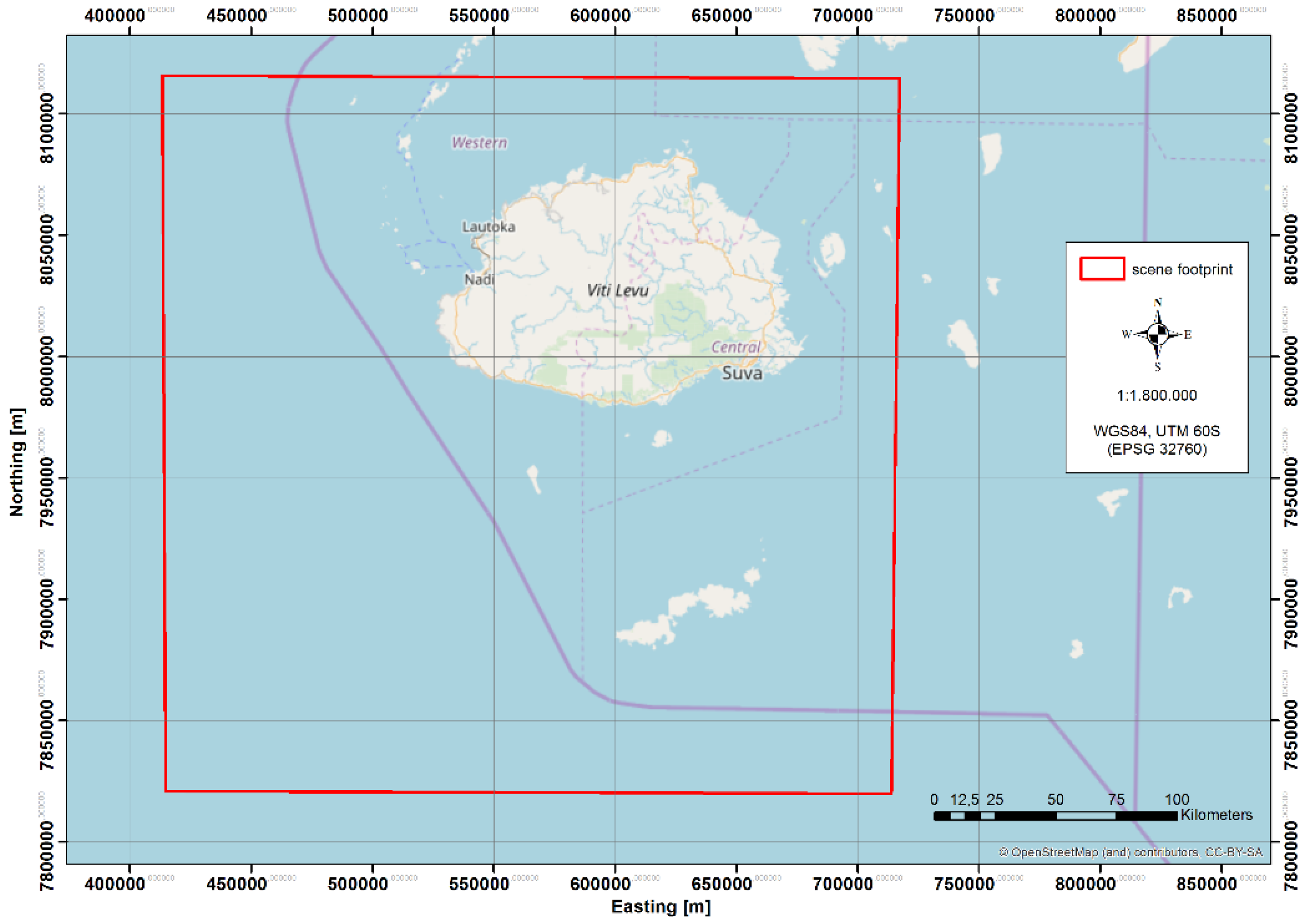
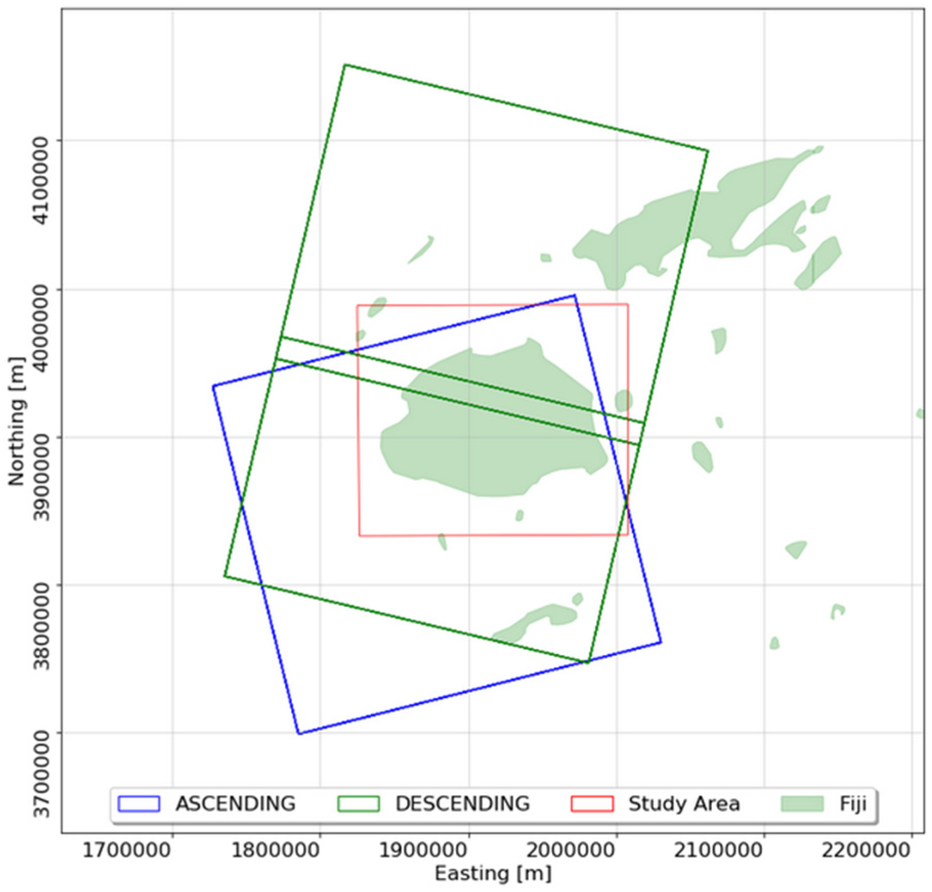
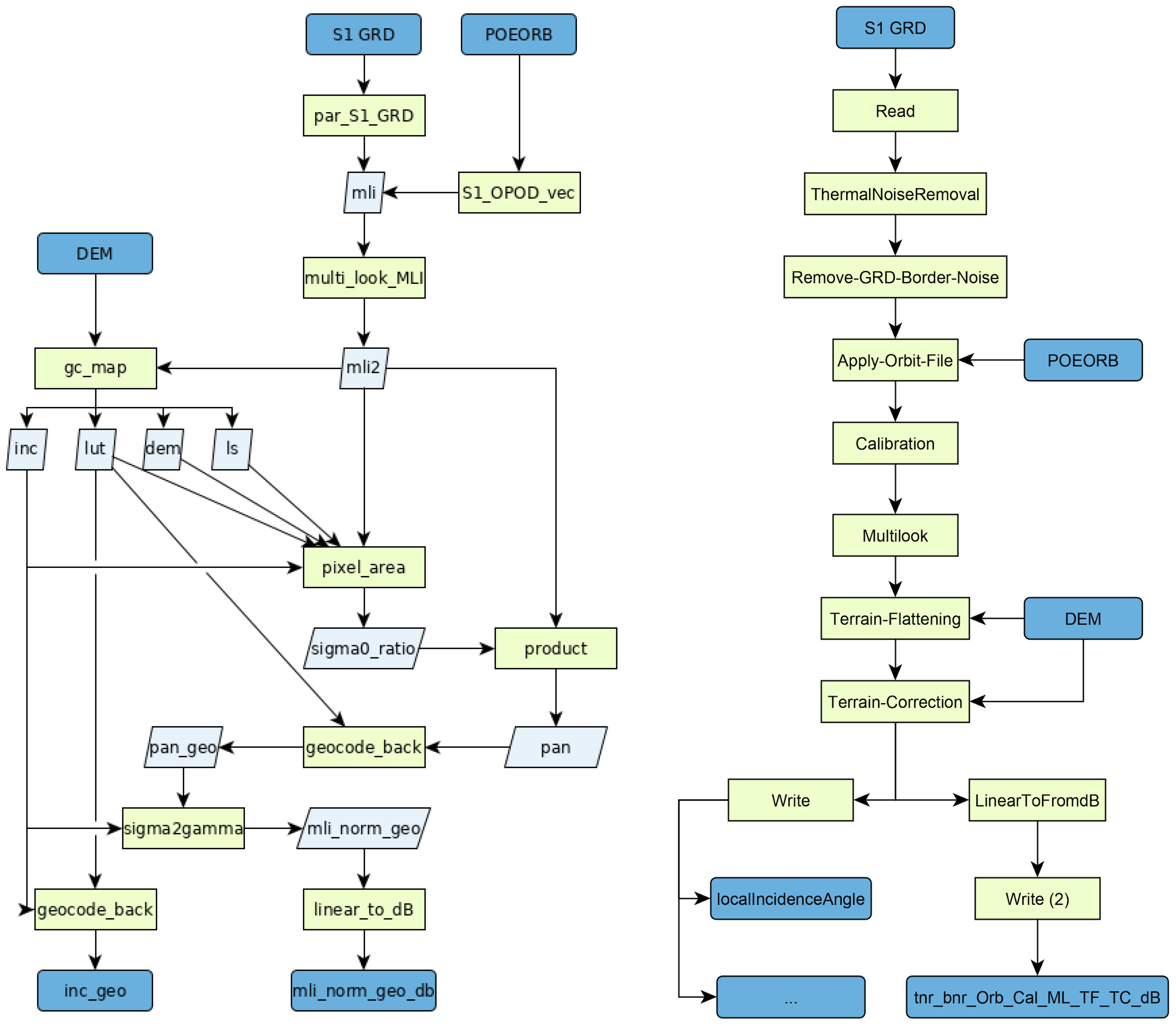
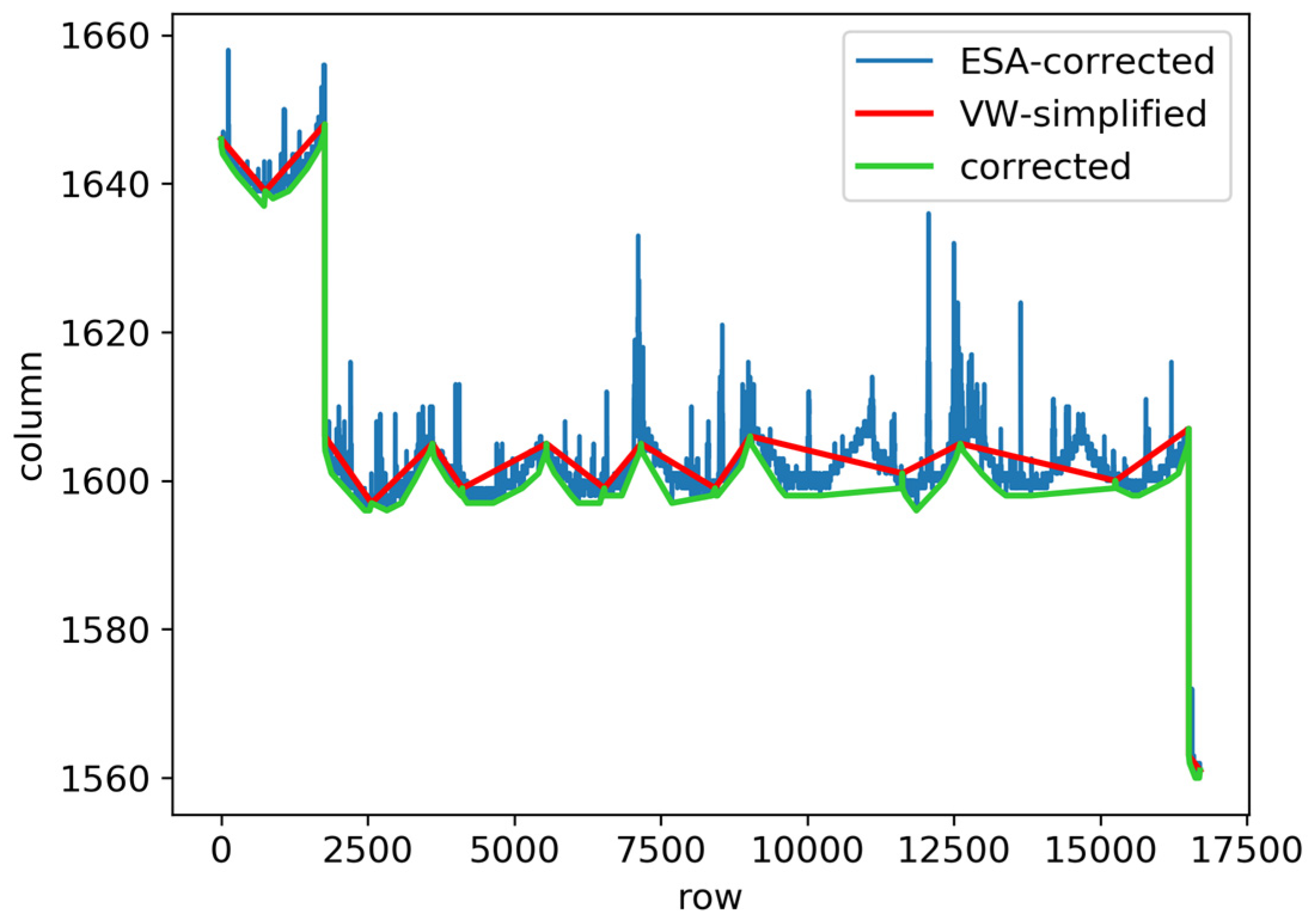
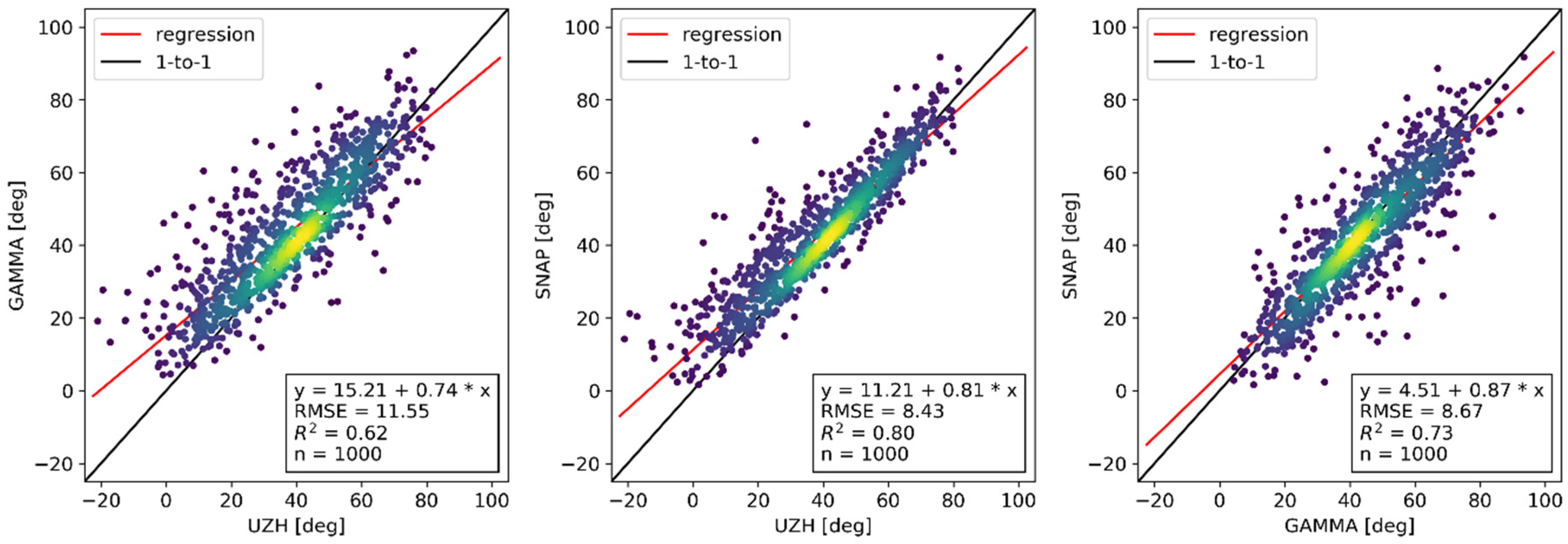
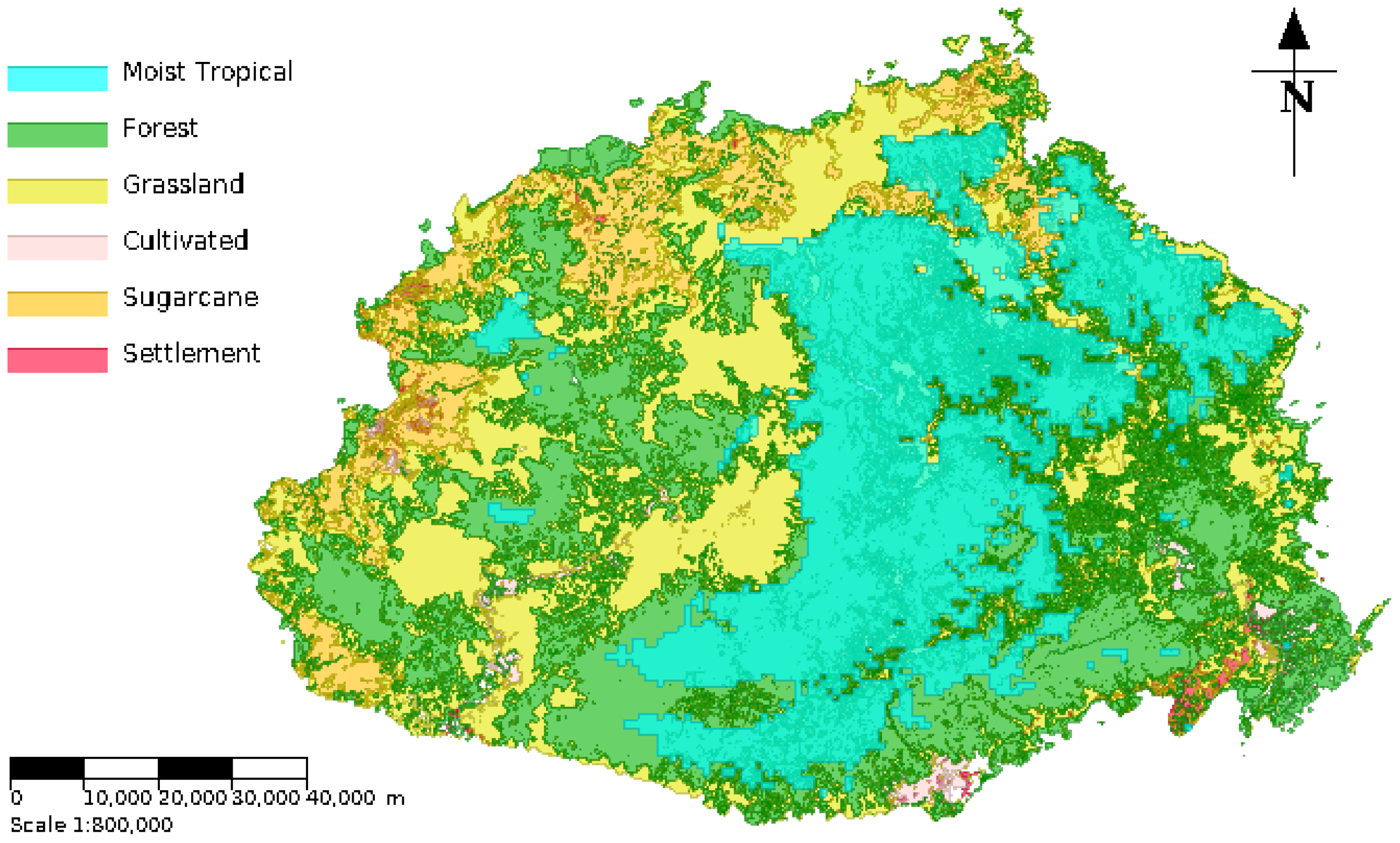
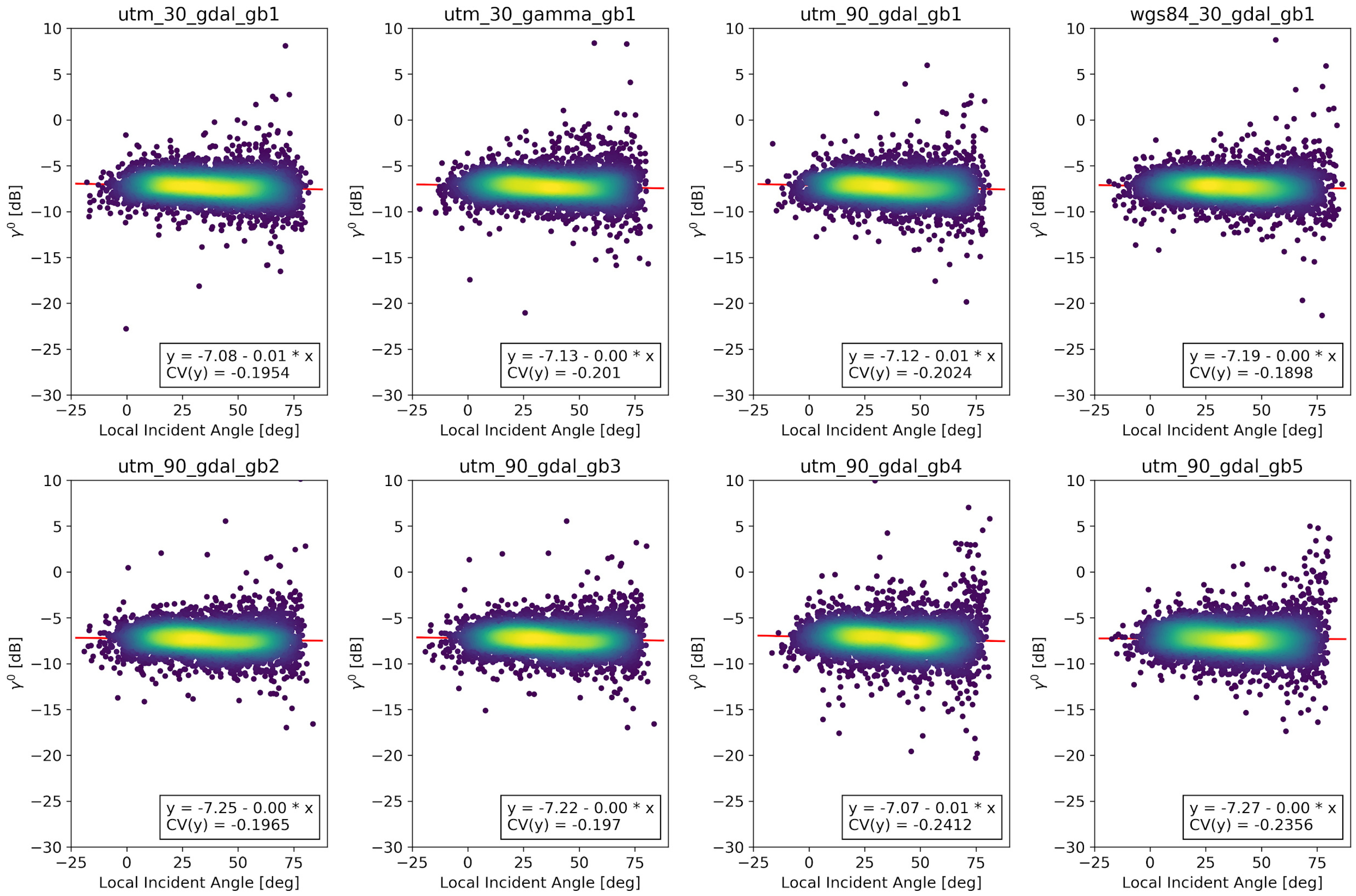
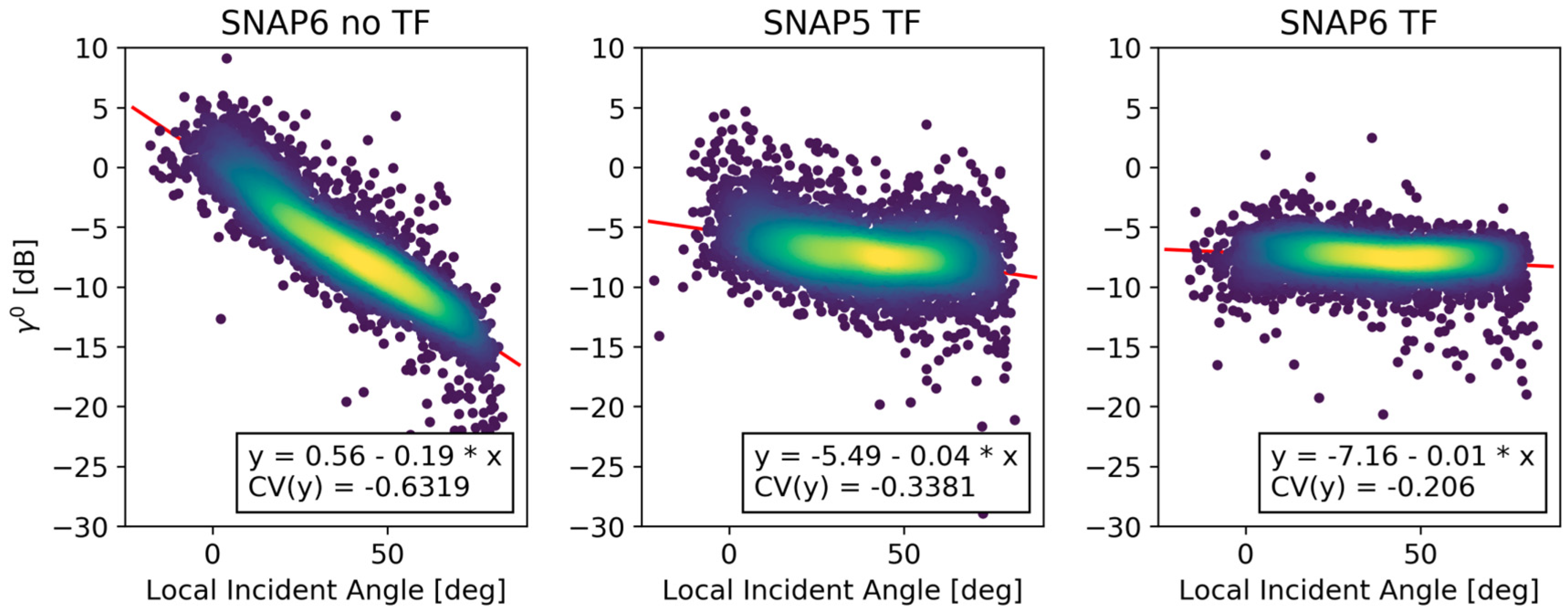
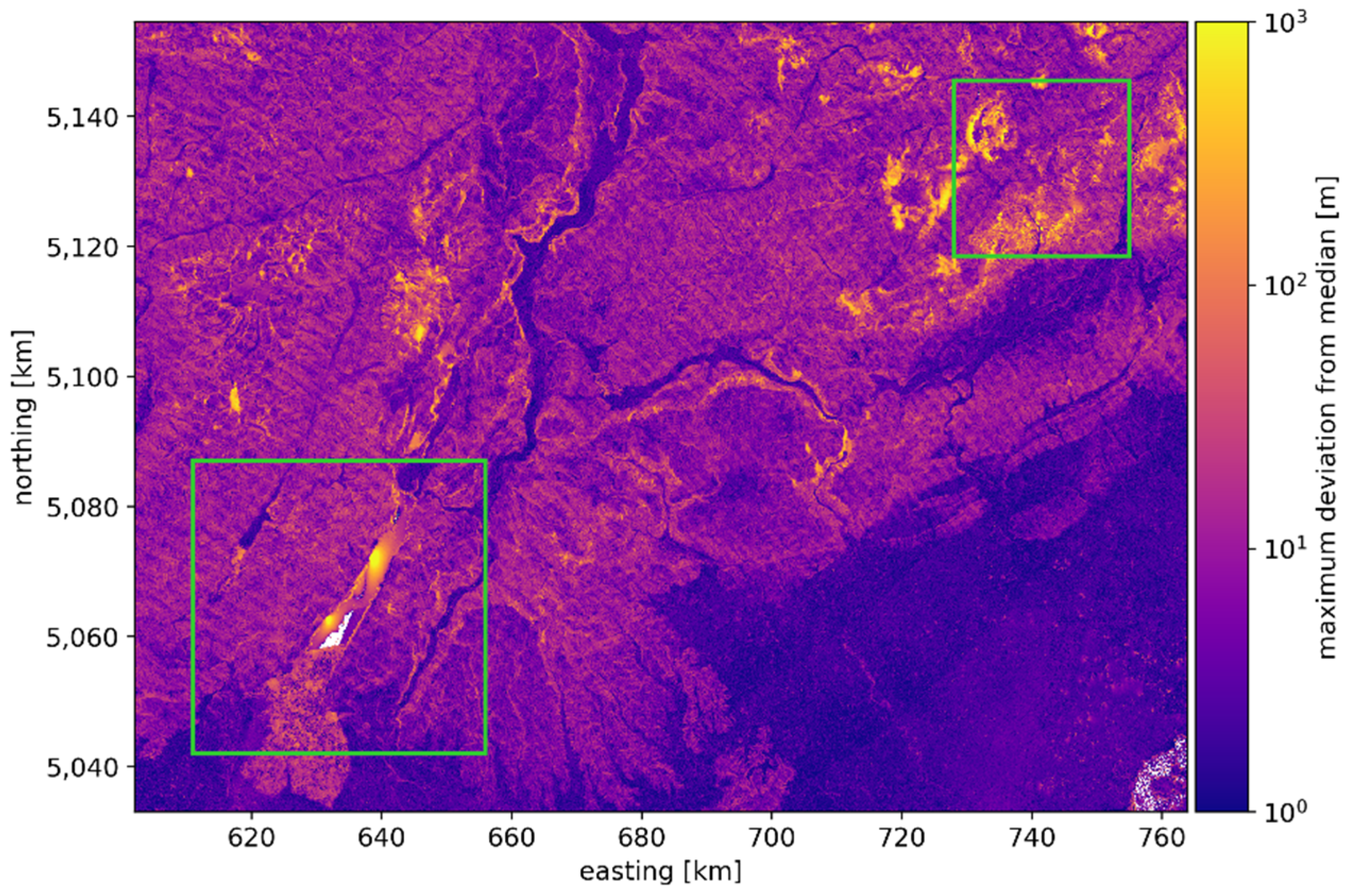
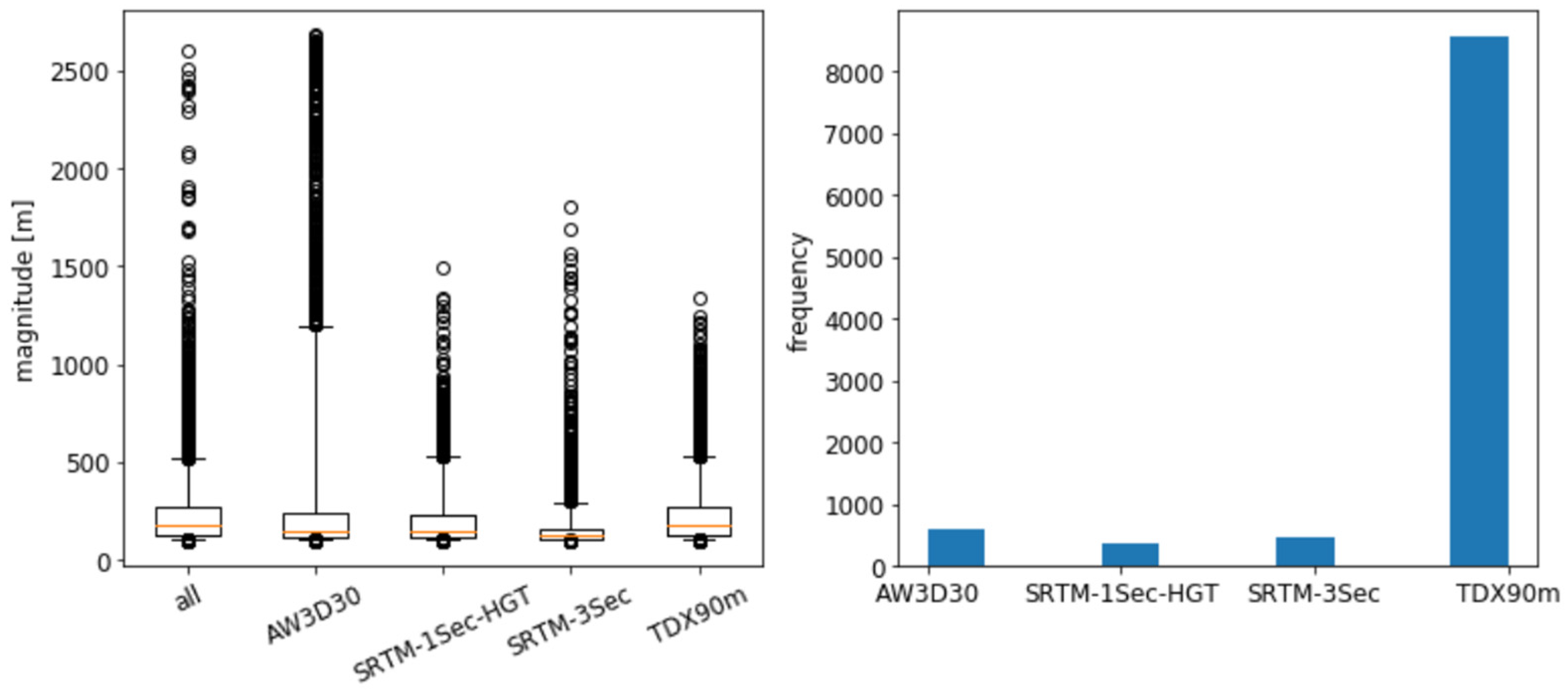
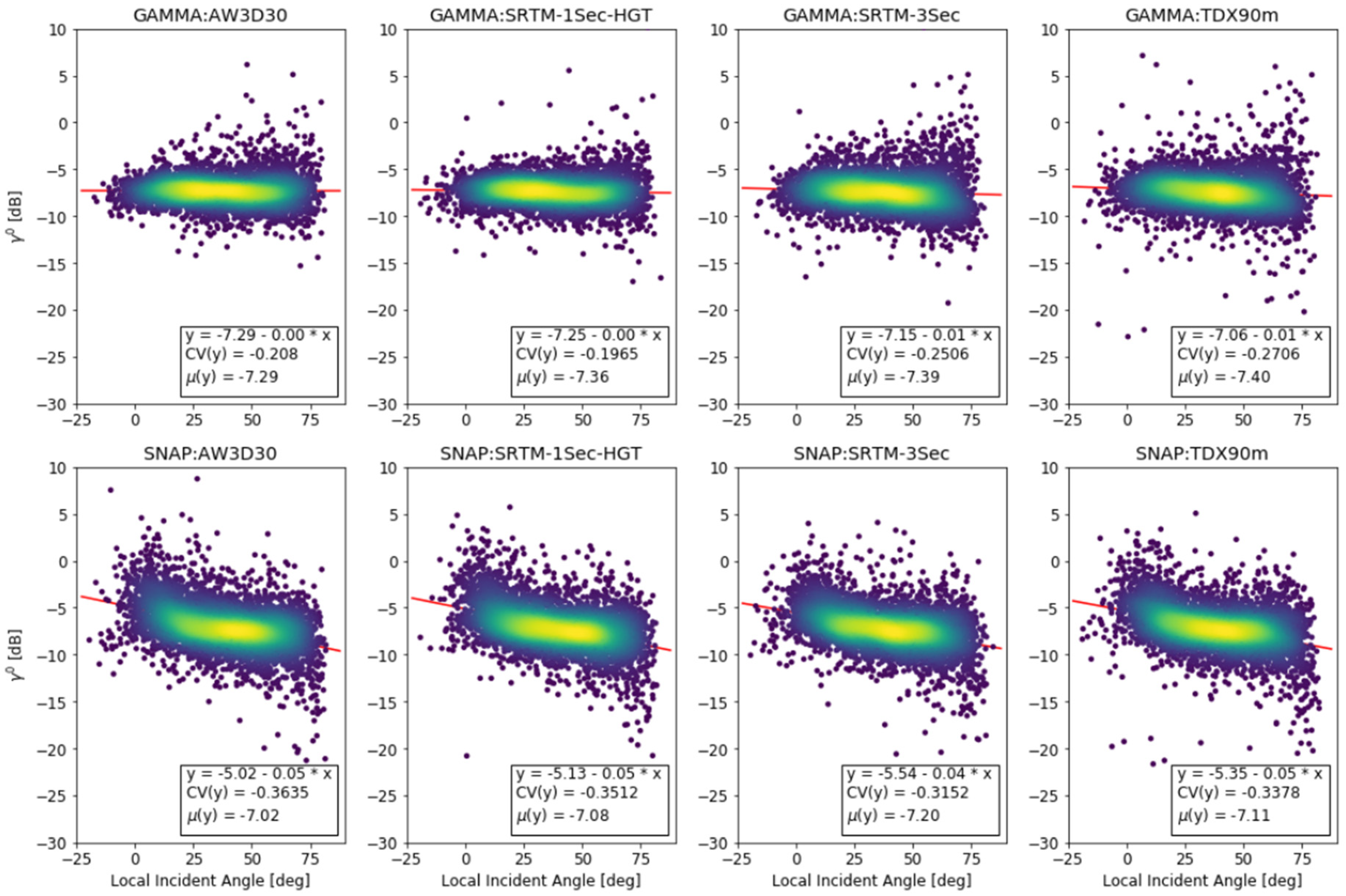
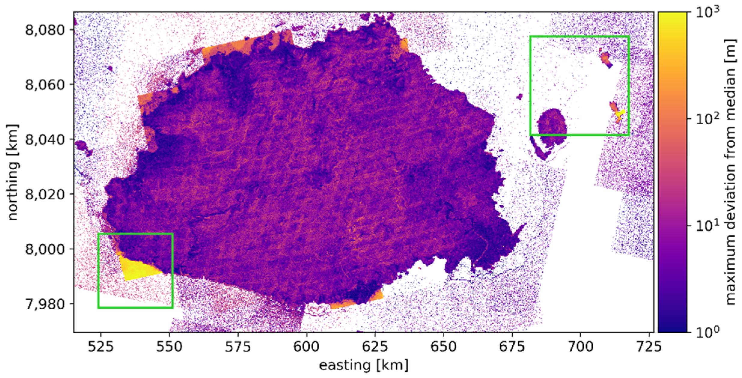
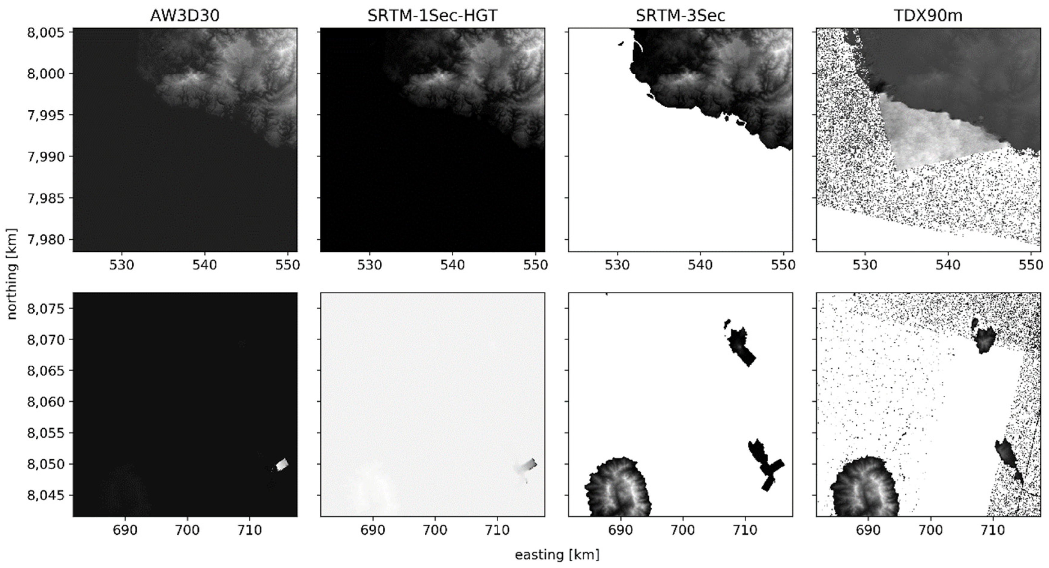
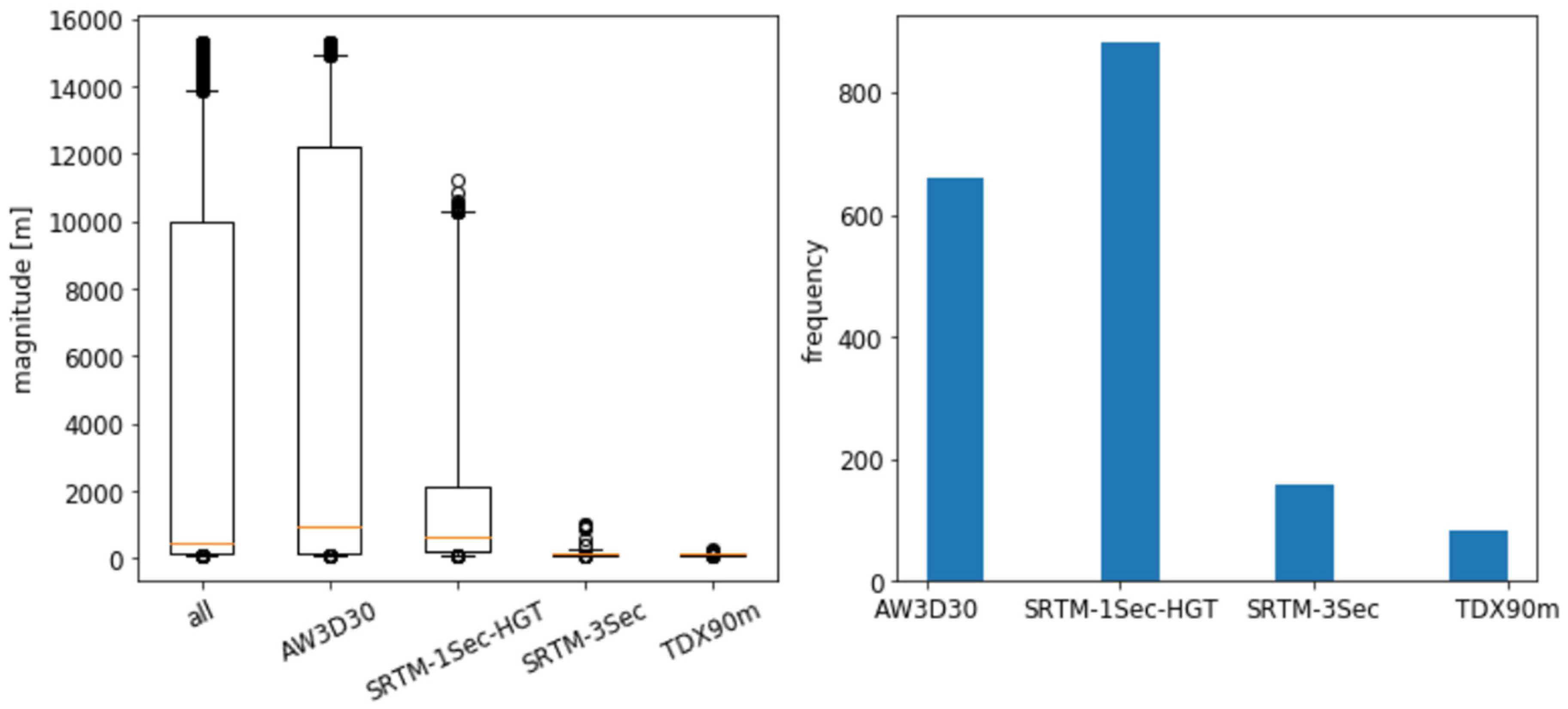
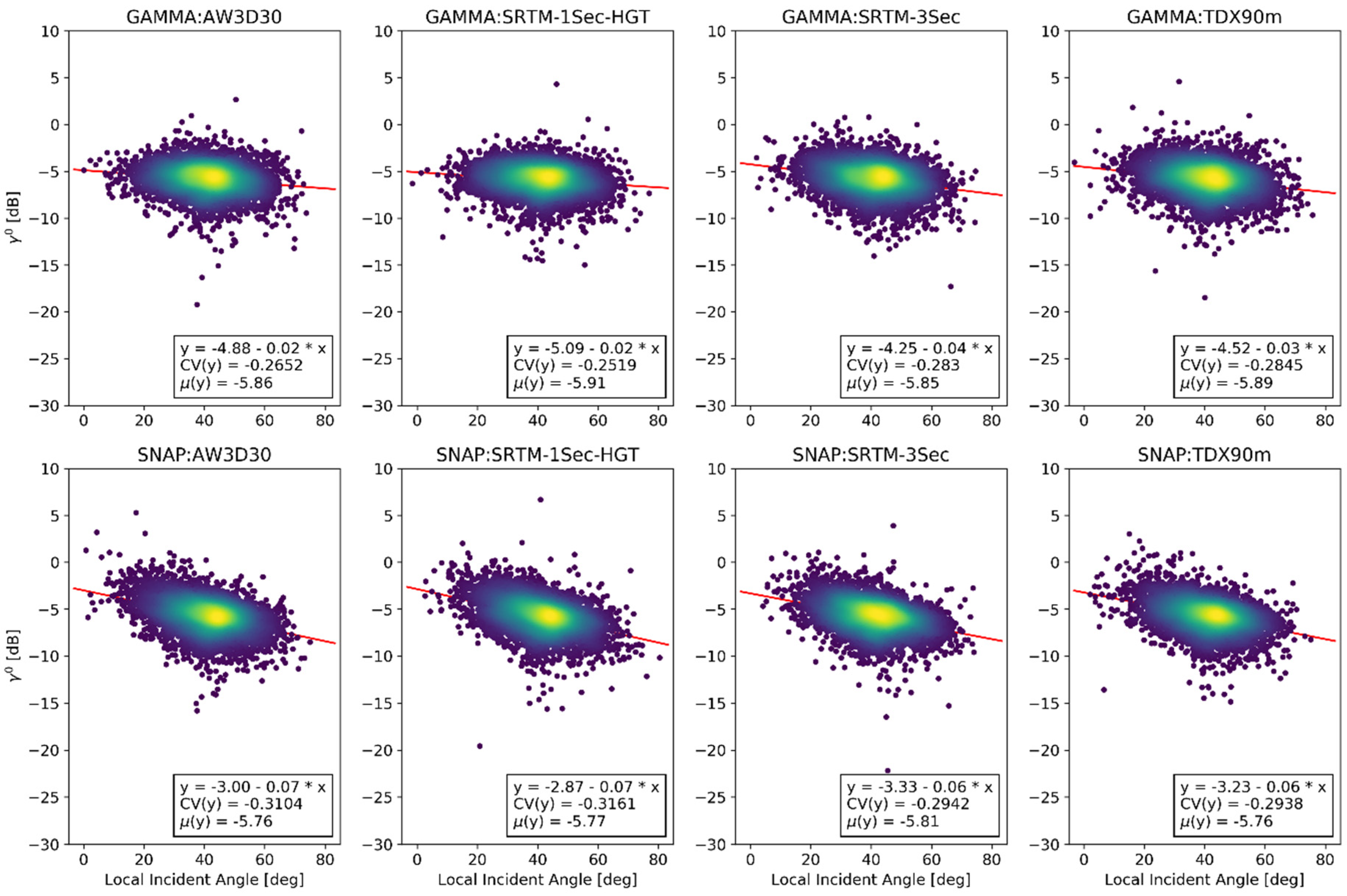
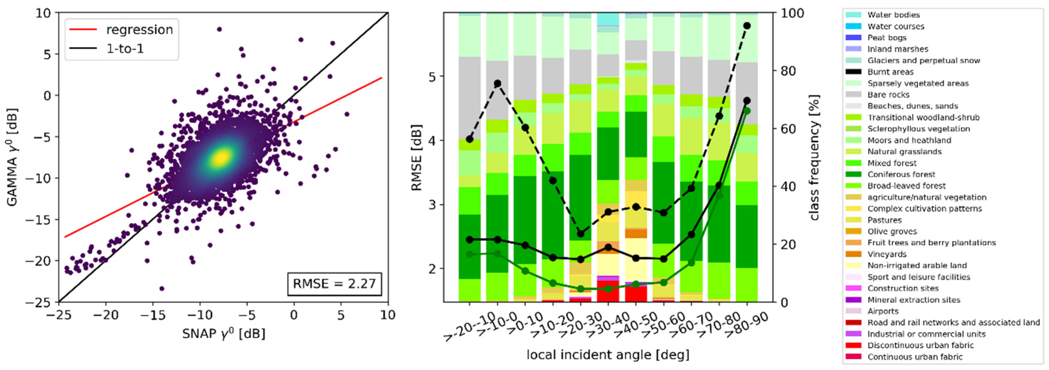
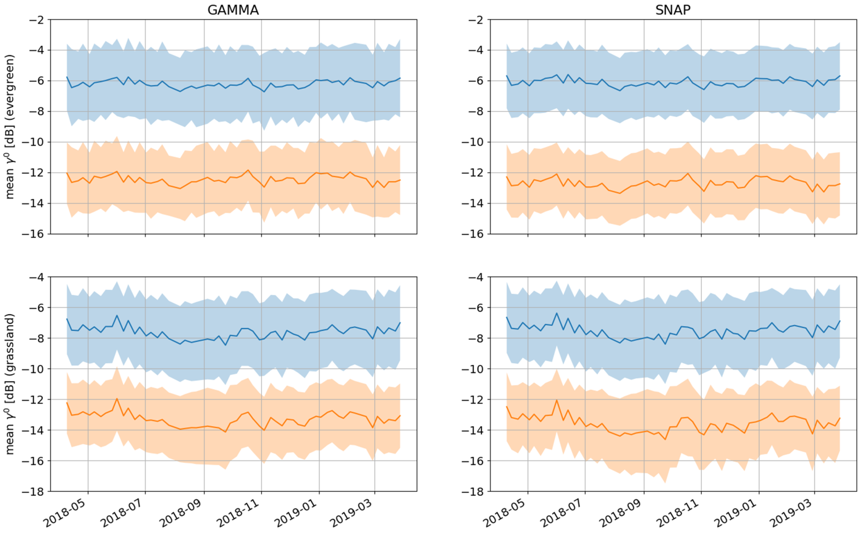
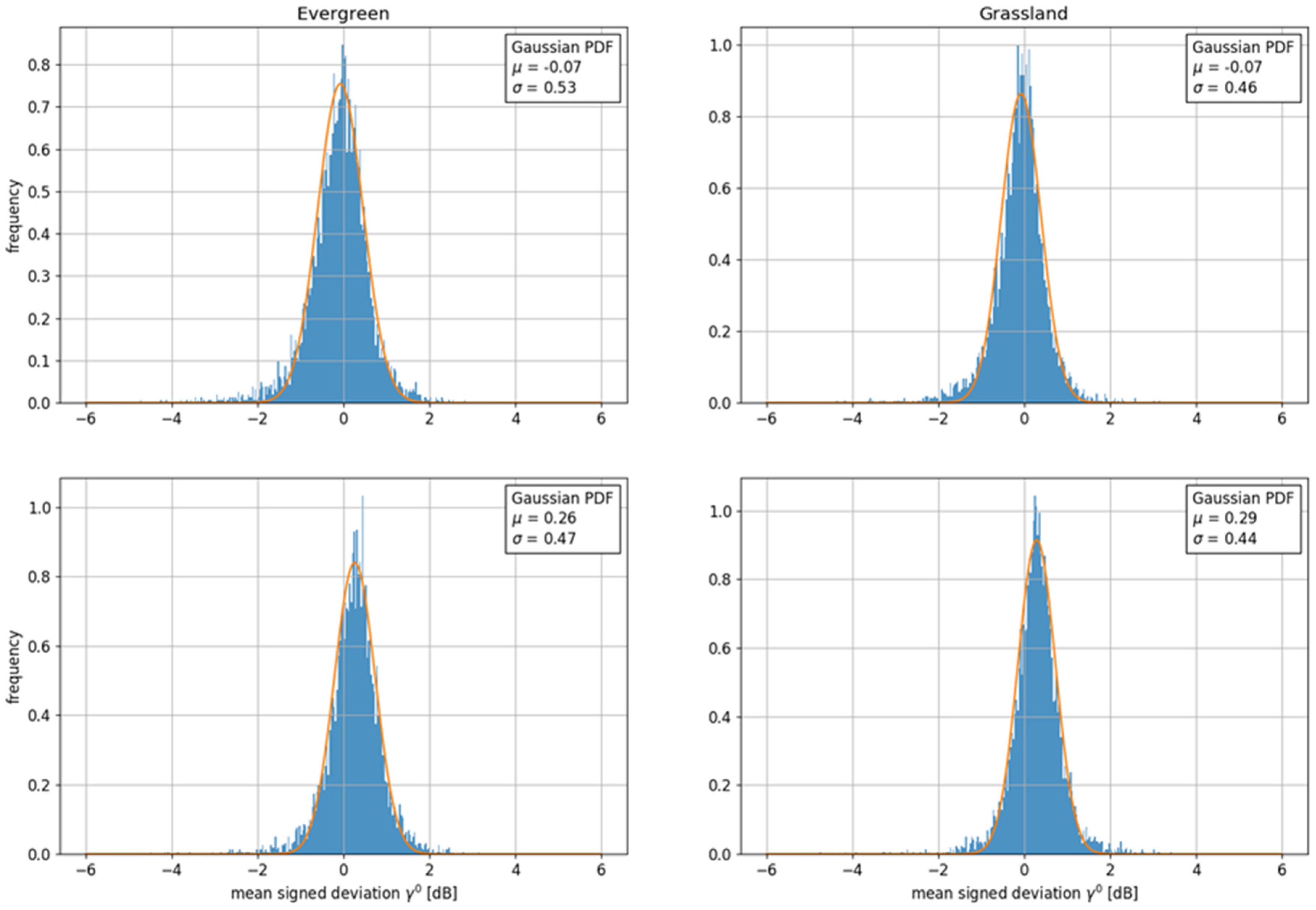
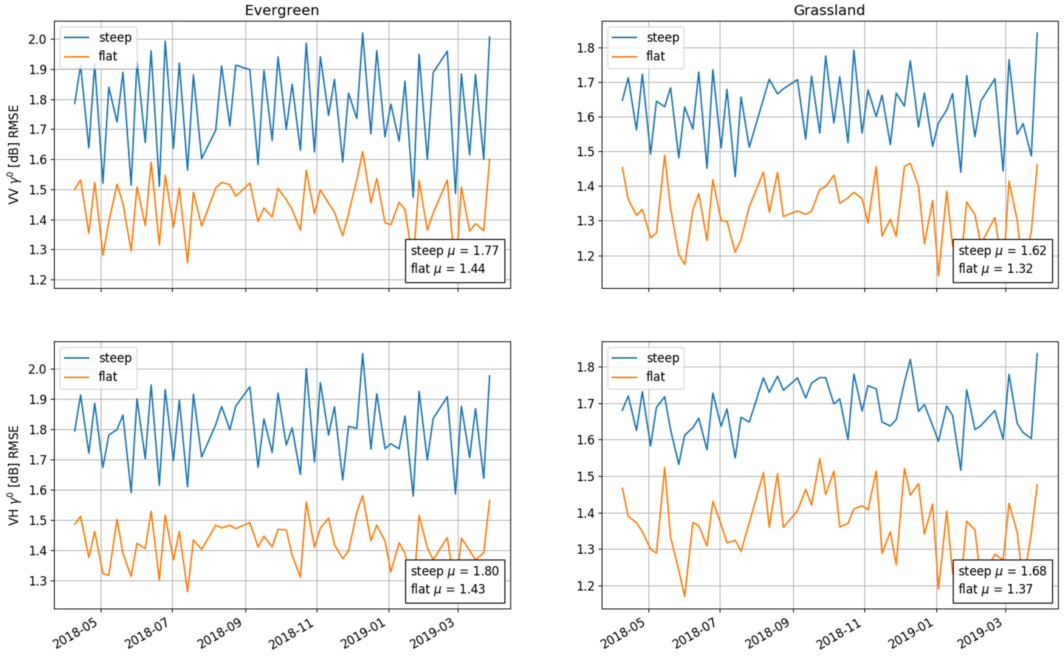
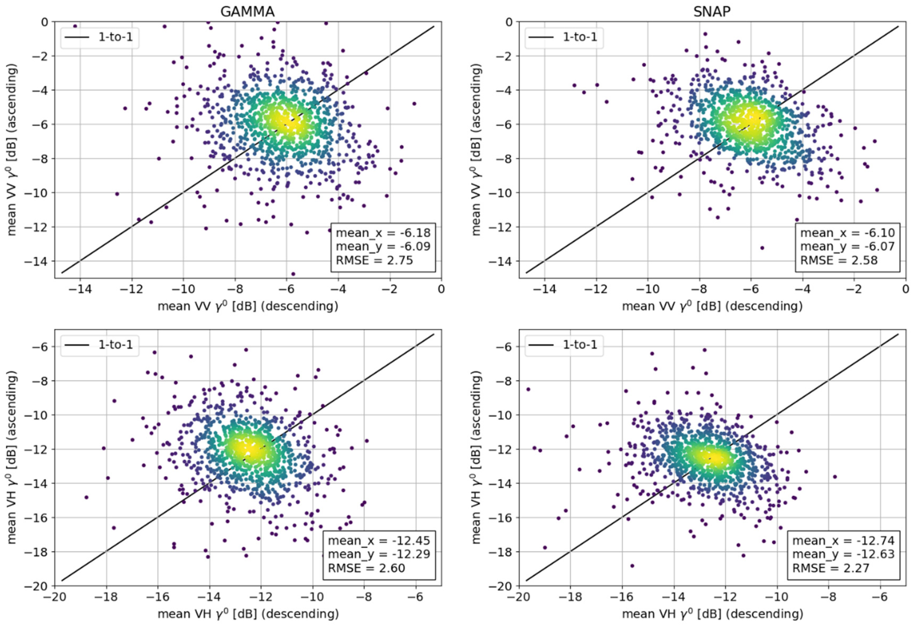