Identifying GNSS Signals Based on Their Radio Frequency (RF) Features—A Dataset with GNSS Raw Signals Based on Roof Antennas and Spectracom Generator


Abstract
:1. Introduction and Motivation
2. Related Work to RFF
3. Data Description
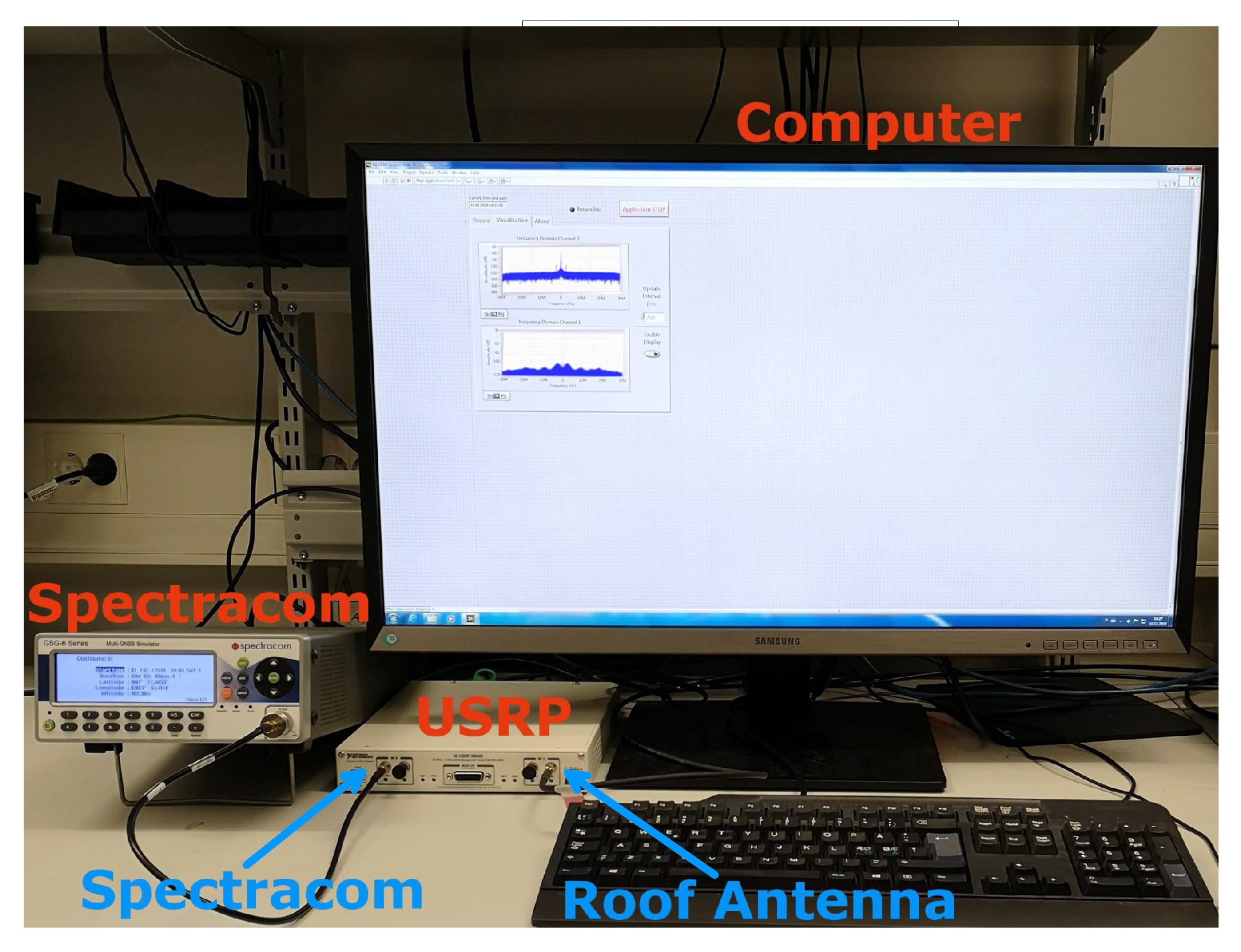
3.1. Laboratory Setup
- Spectracom GSG-64: A multi-frequency and multi-system GNSS signal generator.
- USRP RIO 2954R: Software-defined radio platform, two receive channels with 80 MHz/channel 70 of real-time bandwidth. It has a MXI-Express kit (PCI-based PXI controllers +x4 MXI-Express).
- Lenovo P510 computer: Host computer (Intel Xeon CPU E3-1225 v5 @ 3.30 GHz, 32GB RAM, 256 GB SSD hard disk).
- Tallysman TW3972 and Novatel GPS-703-GGG antennas: Triple Band GNSS Antennas placed on the roof.
3.2. Measurement Parameters
3.3. Measurement Scenarios
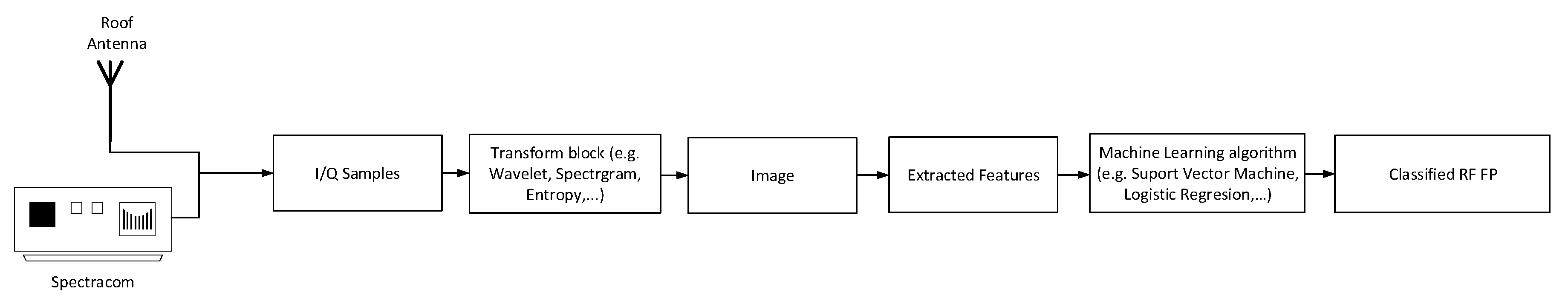
4. Examples of Data Analysis
4.1. Transforms for RF FP Feature Extraction
4.1.1. Wavelet Transform
4.1.2. Spectrogram
4.1.3. Wigner-Ville Distribution
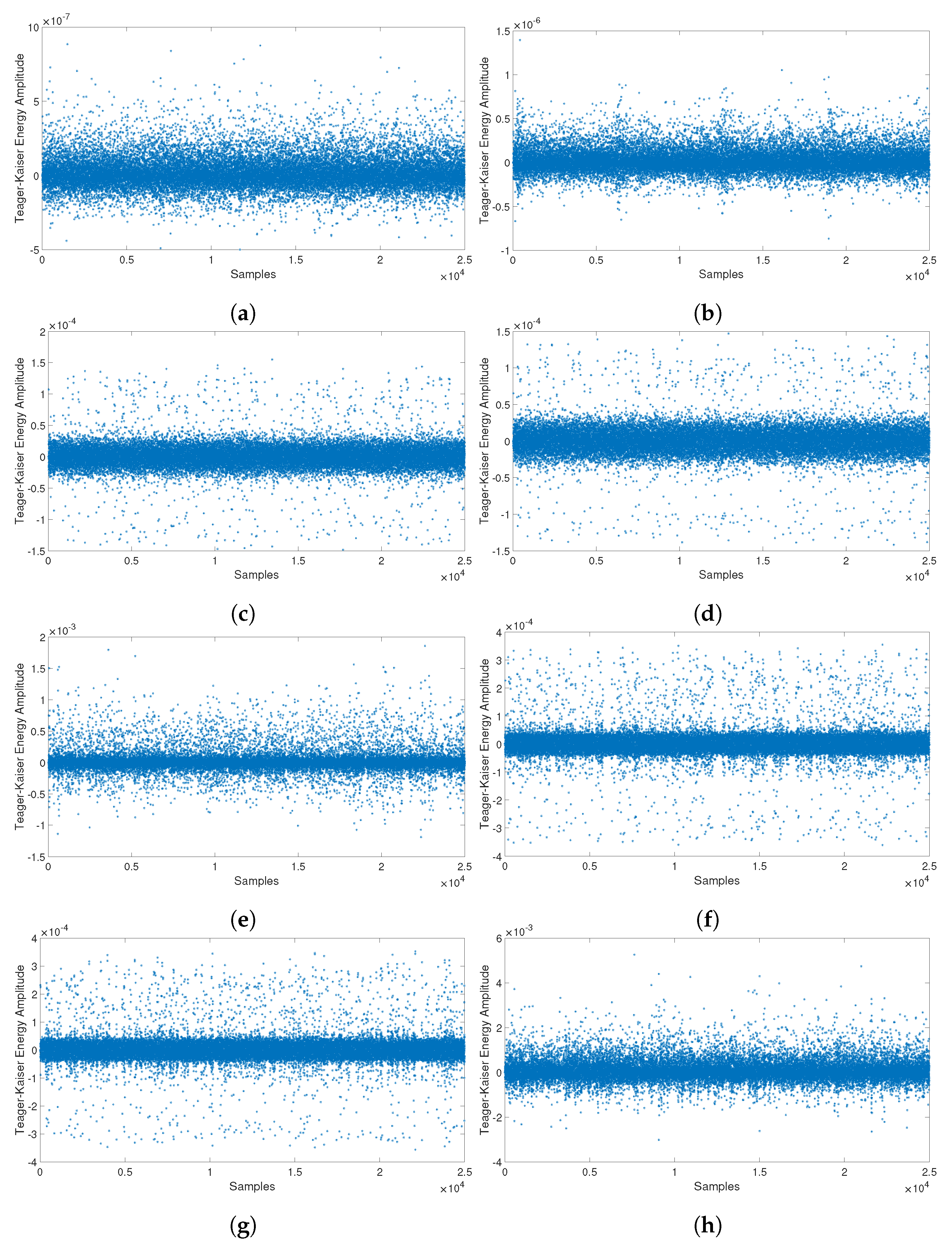
4.1.4. Teager-Kaiser Energy Operator
4.2. Machine Learning for RF FP Classification
4.2.1. Logistic Regression
4.2.2. Support Vector Machine
- linear kernel: ;
- polynomial kernel: , d is the order;
- Gaussian kernel (or ’rbf’): ;
- sigmoid kernel: , and .
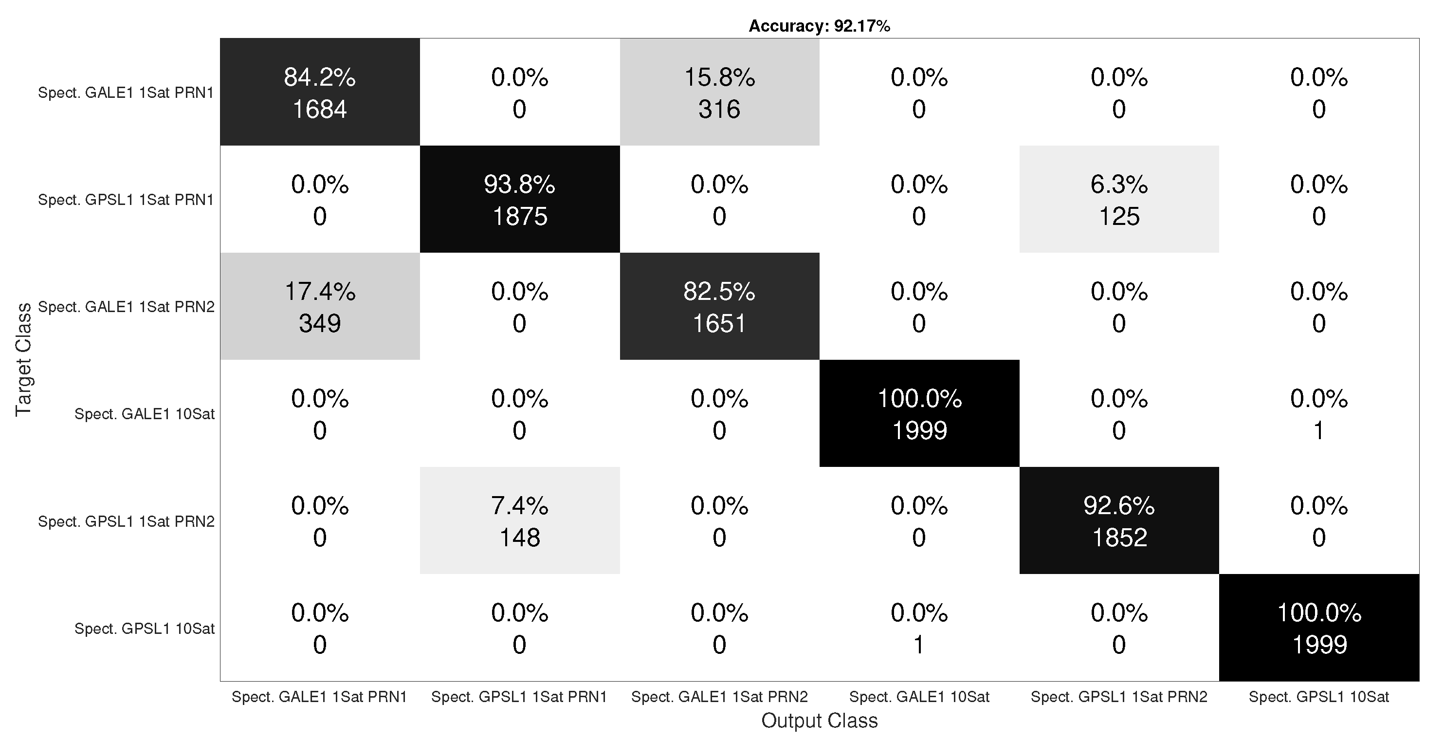
4.3. Results
5. Conclusions and Open Directions
6. Dataset Repository And License
Author Contributions
Funding
Acknowledgments
Conflicts of Interest
Abbreviations
| ADC | Analog-to-Digital Converter |
| BLE | Bluetooth Low Energy |
| CNN | Convolutional Neural Networks |
| CWT | Continuous Wavelet Transform |
| DWT | Discrete Wavelet Transform |
| FP | Fingerprinting |
| GPS | Global Positioning System |
| GNSS | Global Navigation Satellite Systems |
| IF | Intermediate Frequency |
| IoT | Internet of Things |
| LR | Logistic Regression |
| LPF | Logistic Probability Function |
| PE | Permutation Entropy |
| PPS | Pulse-Per-Second |
| PRN | Pseudo-Random Number |
| RF | Radio Frequency |
| RFF | Radio Frequency Fingerprinting |
| SDR | Software Defined Radio |
| SMA | SubMiniature version A |
| STFT | Short-Time Fourier transform |
| SVM | Support Vector Machine |
| TK | Teager-Kaiser |
| TKEO | Teager-Kaiser energy operator |
| USRP | Universal Software Radio Peripheral |
| WLAN | Wireless Local Area Networks |
| WVD | Wigner-Ville distribution |
References
- Bertoncini, C.; Rudd, K.; Nousain, B.; Hinders, M. Wavelet Fingerprinting of Radio-Frequency Identification (RFID) Tags. IEEE Trans. Ind. Electron. 2012, 59, 4843–4850. [Google Scholar] [CrossRef]
- Patel, H.J.; Temple, M.A.; Baldwin, R.O. Improving ZigBee Device Network Authentication Using Ensemble Decision Tree Classifiers With Radio Frequency Distinct Native Attribute Fingerprinting. IEEE Trans. Reliab. 2015, 64, 221–233. [Google Scholar] [CrossRef]
- Sankhe, K.; Belgiovine, M.; Zhou, F.; Angioloni, L.; Restuccia, F.; D’Oro, S.; Melodia, T.; Ioannidis, S.; Chowdhury, K. No Radio Left Behind: Radio Fingerprinting Through Deep Learning of Physical-Layer Hardware Impairments. IEEE Trans. Cogn. Commun. Netw. 2019, 1. [Google Scholar] [CrossRef]
- Aghnaiya, A.; Ali, A.M.; Kara, A. Variational Mode Decomposition-Based Radio Frequency Fingerprinting of Bluetooth Devices. IEEE Access 2019, 7, 144054–144058. [Google Scholar] [CrossRef]
- Ali, A.M.; Uzundurukan, E.; Kara, A. Assessment of Features and Classifiers for Bluetooth RF Fingerprinting. IEEE Access 2019, 7, 50524–50535. [Google Scholar] [CrossRef]
- Borio, D.; Gioia, C.; Cano Pons, E.; Baldini, G. GNSS Receiver Identification Using Clock-Derived Metrics. Sensors 2017, 17, 2120. [Google Scholar] [CrossRef] [PubMed] [Green Version]
- Shi, Z.; Liu, M.; Huang, L. Transient-based identification of 802.11b wireless device. In Proceedings of the 2011 International Conference on Wireless Communications and Signal Processing (WCSP), Nanjing, China, 9–11 November 2011; pp. 1–5. [Google Scholar] [CrossRef]
- Hu, N.; Yao, Y. Identification of legacy radios in a cognitive radio network using a radio frequency fingerprinting based method. In Proceedings of the 2012 IEEE International Conference on Communications (ICC), Ottawa, ON, Canada, 10–15 June 2012; pp. 1597–1602. [Google Scholar] [CrossRef]
- Ali, A.M.; Uzundurukan, E.; Kara, A. Improvements on transient signal detection for RF fingerprinting. In Proceedings of the 25th Signal Processing and Communications Applications Conference (SIU), Antalya, Turkey, 15–18 May 2017; pp. 1–4. [Google Scholar] [CrossRef]
- Köse, M.; Taşcioğlu, S.; Telatar, Z. RF Fingerprinting of IoT Devices Based on Transient Energy Spectrum. IEEE Access 2019, 7, 18715–18726. [Google Scholar] [CrossRef]
- Riyaz, S.; Sankhe, K.; Ioannidis, S.; Chowdhury, K. Deep learning convolutional neural networks for radio identification. IEEE Commun. Mag. 2018, 56, 146–152. [Google Scholar] [CrossRef]
- Xu, Q.; Zheng, R.; Saad, W.; Han, Z. Device fingerprinting in wireless networks: Challenges and opportunities. IEEE Commun. Surv. Tutor. 2015, 18, 94–104. [Google Scholar] [CrossRef] [Green Version]
- Deng, S.; Huang, Z.; Wang, X.; Huang, G. Radio frequency fingerprint extraction based on multidimension permutation entropy. Int. J. Antennas Propag. 2017, 2017, 6. [Google Scholar] [CrossRef] [Green Version]
- An Open Source Global Navigation Satellite Systems Software-Defined Receiver. Available online: https://gnss-sdr.org/ (accessed on 19 December 2019).
- TRIMBLE GNSS Planning Online. Available online: https://www.gnssplanning.com/ (accessed on 19 December 2019).
- Lilly, J.M.; Olhede, S.C. Generalized Morse wavelets as a superfamily of analytic wavelets. IEEE Trans. Signal Process. 2012, 60, 6036–6041. [Google Scholar] [CrossRef] [Green Version]
- Lilly, J.M. Element analysis: A wavelet-based method for analysing time-localized events in noisy time series. Proc. R. Soc. A Math. Phys. Eng. Sci. 2017, 473, 20160776. [Google Scholar] [CrossRef] [PubMed]
- Mallat, S.G. A theory for multiresolution signal decomposition: The wavelet representation. IEEE Trans. Pattern Anal. Mach. Intell. 1989, 7, 674–693. [Google Scholar] [CrossRef] [Green Version]
- Mitra, S.K.; Kuo, Y. Digital Signal Processing: A Computer-Based Approach; McGraw-Hill: New York, NY, USA, 2006; Volume 2. [Google Scholar]
- Oppenheim, A.V. Discrete-Time Signal Processing; Pearson Education India: Bengaluru, India, 1999. [Google Scholar]
- Ferre, R.M.; Wang, W.; Lohan, E.S. Identifying GNSS transmitters based on their RadioFrequency (RF) features—A dataset with GNSS roofantenna and Spectracom-based GNSS signals. Zenodo 2020, in press. [Google Scholar] [CrossRef]


| Sampling Frequency | 50 MSamples/s |
| Quantization Bits | 16 bits |
| Recording Duration | 20 s |
| Approximated File Size per recording | 4 Gb |
| IF | 0 Hz (baseband) |
| Gain | 30 dB |
| Transmit Power per Satellite | −70 dBm |
| Additive White Noise Channel | No-noise |
| Channel Effects | No channel effects |
| Simulated Receiver Movement | Static |
| Tallysman TW3972 | Novatel GPS-703-GGG | |||
|---|---|---|---|---|
| Compatible Constellations | GPS L1/L2/L5, GLONASS G1/G2/G3, BeiDou B1/B2 and Galileo E1/E5a+b | |||
| Noise Figure | 2.5 dB | 2 dB | ||
| Out of Band Rejection | L1/E1/B1/G1 <1450 MHz >30 dB >1690 MHz >30dB >1730 MHz >40 dB | L5/E5/L2/G2 <1050 MHz >45 dB <1125 MHz >30 dB >1350 MHz >45 dB | L1/E1/B1/G1 ± 100 MHz 30 dBc | L5/E5/L2/G2 ± 200 MHz 50 dBc |
| LNA Gain | 37 dB | 29 dB | ||
| Filter Bandwidth | L1/E1/B1/G1 1525 MHz–1606 MHz | L5/E5/L2/G2 1164 MHz–1254 MHz | L1/B1/E1/G1 1551.5 MHz–1608.5 MHz | L5/E5/L2/G2 1165.5 MHz–1238.5 MHz |
| Dimensions | 66 mm diameter × 21 mm | 185 mm diameter × 69 mm | ||
| Device | Scenario ID | Constellation | Amount of Satellites |
|---|---|---|---|
| Antenna Tallysman | A1 | GPS L1 + GALILEO E1 + BeiDou B1 | Variable according to date and time of the recording * |
| A3 | GPS L5 + GALILEO E5 + BeiDou B2 | Variable according to date and time of the recording * | |
| Antenna Novatel | A2 | GPS L1 + GALILEO E1 + BeiDou B1 | Variable according to date and time of the recording * |
| A4 | GPS L5 + GALILEO E5 + BeiDou B2 | Variable according to date and time of the recording * | |
| Spectracom | S1–S9 | GPS L1 | 1 (7 recordings with different PRN), 5 and 10 |
| S10–S18 | GPS L5 | 1 (7 recordings with different PRN), 5 and 10 | |
| S19–S27 | GALILEO E1 | 1 (7 recordings with different PRN), 5 and 10 | |
| S28–S36 | GALILEO E5 | 1 (7 recordings with different PRN), 5 and 10 | |
| S37–S45 | GLONASS G1 | 1 (7 recordings with different PRN), 5 and 10 | |
| S46–S54 | BeiDou B1 | 1 (7 recordings with different PRN), 5 and 10 | |
| S55–S56 | GPS L1 + GALILEO E1 + BeiDou B1 | 1 and 5 per constellation | |
| S57–S58 | GPS L1 + GALILEO E1 + BeiDou B1 + GLONASS G1 | 1 and 5 per constellation |
© 2020 by the authors. Licensee MDPI, Basel, Switzerland. This article is an open access article distributed under the terms and conditions of the Creative Commons Attribution (CC BY) license (http://creativecommons.org/licenses/by/4.0/).
Share and Cite
Morales-Ferre, R.; Wang, W.; Sanz-Abia, A.; Lohan, E.-S. Identifying GNSS Signals Based on Their Radio Frequency (RF) Features—A Dataset with GNSS Raw Signals Based on Roof Antennas and Spectracom Generator. Data 2020, 5, 18. https://0-doi-org.brum.beds.ac.uk/10.3390/data5010018
Morales-Ferre R, Wang W, Sanz-Abia A, Lohan E-S. Identifying GNSS Signals Based on Their Radio Frequency (RF) Features—A Dataset with GNSS Raw Signals Based on Roof Antennas and Spectracom Generator. Data. 2020; 5(1):18. https://0-doi-org.brum.beds.ac.uk/10.3390/data5010018
Chicago/Turabian StyleMorales-Ferre, Ruben, Wenbo Wang, Alejandro Sanz-Abia, and Elena-Simona Lohan. 2020. "Identifying GNSS Signals Based on Their Radio Frequency (RF) Features—A Dataset with GNSS Raw Signals Based on Roof Antennas and Spectracom Generator" Data 5, no. 1: 18. https://0-doi-org.brum.beds.ac.uk/10.3390/data5010018