Experimental Force Data of a Restrained ROV under Waves and Current

Abstract

Hydrodynamic forces are an important input value for the design, navigation and station keeping of underwater Remotely Operated Vehicles (ROVs). The experiment investigated the forces imparted by currents (with representative real world turbulence) and waves on a commercially available ROV, namely the BlueROV2 (Blue Robotics, Torrance, USA). Three different distances of a simplified cylindrical obstacle (shading effects) were investigated in addition to the free stream cases. Eight tethers held the ROV in the middle of the 2 m water depth to minimise the influence of the support structure without completely restricting the degrees of freedom (DoF). Each tether was equipped with a load cell and small motions and rotations were documented with an underwater video motion capture system. The paper describes the experimental set-up, input values (current speed and wave definitions) and initial processing of the data. In addition to the raw data, a processed dataset is provided, which includes forces in all three main coordinate directions for each mounting point synchronised with the 6DoF results and the free surface elevations. The provided dataset can be used as a validation experiment as well as for testing and development of an algorithm for position control of comparable ROVs.

Dataset:https://0-doi-org.brum.beds.ac.uk/10.7488/ds/2835

1. Introduction

As part of the ORCA Hub project [1,2] (orcahub.org) an experimental investigation of a remotely operated underwater vehicle (ROV) was conducted in the FloWave wave and current facility, located at the University of Edinburgh. Gabl et al. [3] provides a thorough analysis of the experimental outputs and the complete dataset is available via DataShare Edinburgh [4].

Previous comparable investigations had profoundly different experimental set-ups from the one presented in this manuscript. Generally they used a towing tank, where the forces on the underwater vehicle were created by attaching the vehicle to a movable gantry and moving the gantry at different speeds [5]. Flumes have also been utilised, by securing the ROV through a bending mechanism and measuring the bending forces through load cells for various flow rates [6]. Alternatively, rather than restricting the movement of the ROV, experiments have been conducted by lowering the ROV using a cable and monitoring the rotation induced by disturbances [7]. A simpler and more cost efficient experimental procedure is the free-decay pendulum test, which utilises minimal apparatus to infer hydrodynamic parameters. The ROV or a scaled model is attached to one end of a pendulum, which is then displaced from an equilibrium position and the decay of amplitude is observed [8,9]. Different test classes may result in different identified parameters; a study was conducted in [10] to investigate this element, comparing a towing tank test to an open water self propelled test.

Some other studies focused on more theoretical problems, such as shallow wave forces on submerged thin plates [11,12]; or on modelling the control of a submerged vehicles, but taking into account disturbances derived from currents [13]. Strip theory has also been applied to estimate forces acting on underwater vehicles whilst operating in shallow water where the influence of sea waves is prevalent. However, it should be noted that this procedure is only an accurate representation for slender bodies [14,15]. Computational Fluid Dynamics (CFD) is another numerical method that can offer estimations of parameters, but demonstrates limitations such as neglecting the effect of movement within a non-constant flow [16,17].

The present document offers the results of a comprehensive set of experiments, encompassing motion control and evaluation of disturbances introduced by currents, waves and surrounding submerged structures. A very similar approach by Dukan et al. [18] tested their dynamic positioning system in open waters, not considering the influence of other submerged structures.

The aim of the presented investigation was to quantify the hydrodynamic forces on a ROV, both when passively subjected to currents and waves and when the propellers of the ROV were activated. The latter experiment was repeated for different rotation speeds of the propellers. A frame was built to hold the ROV at mid-depth with eight tethers, designed to keep shadowing and other local influences from the support frame to a minimum. Each individual line was equipped with a load cell to capture the ROV restraining forces. The unique facility at FloWave [19,20] allows the investigation of waves and current combined in any direction. The flow speed for this investigation was limited to a maximum of 1 m/s (all velocities are based on previous calibration measurements of the tank at tank centre in 1 m water depth). Furthermore, an obstacle was positioned in front of the ROV at three different distances to investigate different flow shading effects. The collected dataset can be used to test the performance of the ROV, to validate further numerical investigations, and also help develop and refine model-based algorithms for position control which can provide improved performance over classical methods which are currently lacking [21,22].

2. Experimental Set-Up

2.1. Remotely Operated Underwater Vehicle (ROV)

The ROV utilised in these experiments was the BlueROV2, produced by Blue Robotics. The ROV is controllable in five degrees of freedom (DoF) through six T200 thrusters, with four in a horizontal vectored configuration and the remaining two configured vertically; the vehicle cannot be controlled in the pitch unless the heavy configuration is utilised. The dimensions of the vehicle are 0.457 × 0.338 × 0.254 m and it is configured to be positively buoyant with approximately 0.2 kg net buoyancy. Further information is provided by the manufacturer [23].

With regards to alterations from the standard package, the Raspberry Pi 3 was replaced with a NVIDIA Jetson Nano [24] for improved computational power and additional capabilities were added, such as Ping360 Scanning Imaging sonar [25].

2.2. Frame and Obstacle

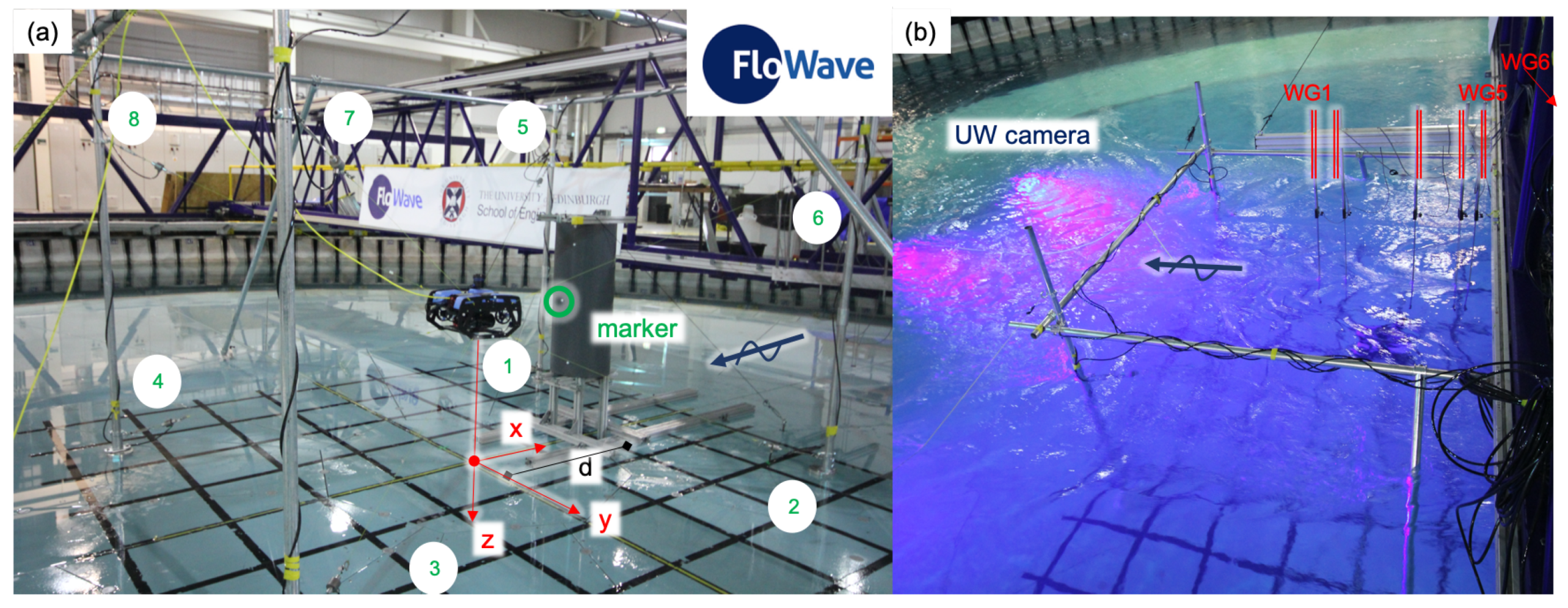
FloWave provides a water depth of 2 m with a 25 m diameter circular basin. 28 flow drives are located in a circle under the tank floor and generate flow speeds of up to 1.6 m/s in any direction. 168 wave makers allow the generation of complex sea states with wave components from any direction. The origin of the measurement coordinate system (global) was located in the centre of the tank on the submered floor. 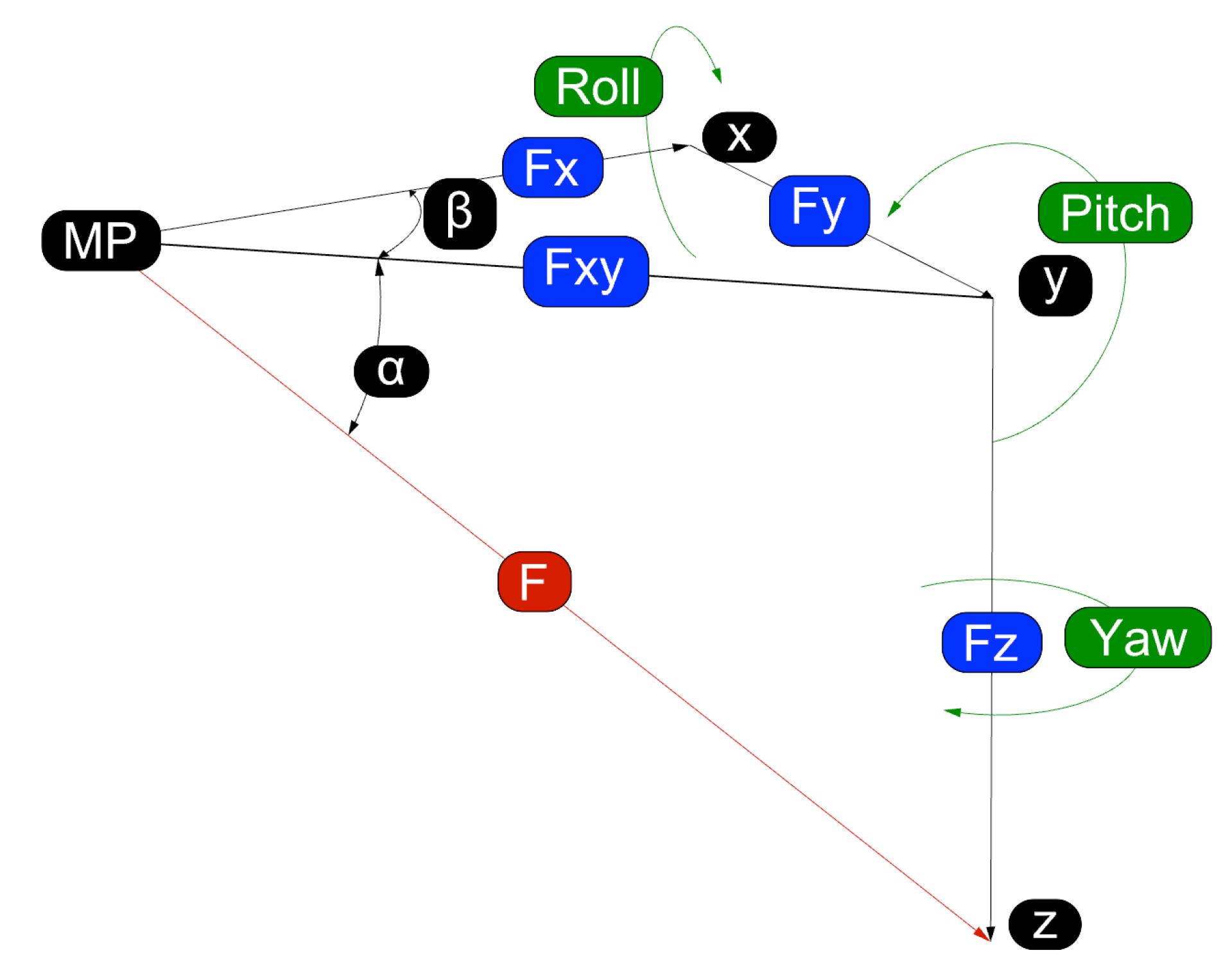A right handed coordinate system was defined with the positive x-axis pointing against the main flow direction and z-axis orientated downwards (Figure 1). The ROV was connected to eight tethers to the frame. The tethers held the ROV at the mid water depth of 1 m from the floor. Galvanised tubes with an outer diameter of 48.3 mm were used to build up the frame. The frame was 3.47 m long in the x-direction, 2.52 m wide in the y-direction and approximately 2.5 m high (surface piercing). The four lower connection points of the tethers to the frame were placed as close to the floor as possible (approximately 120 mm above the floor), with the upper arrangement mirrored around the mid-depth plane. Each tether included one turnbuckle to provide a preload and also one reflective marker, which could be tracked by the motion capturing system. Knowing the position of the ROV, the mounting points (connection of the tether to the ROV) were calculated as virtual points. This allowed the direction of the force vector very accurately determined and three-dimensional force components to be resolved. The collected dataset includes the vectors for each load cell (V) in addition to the main coordinate components. Therefore, the calculated mounting point (MP) is subtracted from the measured frame marker (FP) as following:

$$\overrightarrow{V}=\overrightarrow{FP}-\overrightarrow{MP}$$

(1)

Hence the vectors are pointing away from the ROV. The location of the MP on the ROV are provided in

Table 1. Distance of each mounting point (MP) on the remotely operated underwater vehicle (ROV) in relation to the centre of gravity.

Direction	MP1	MP2	MP3	MP4	MP5	MP6	MP7	MP8
$\Delta x\left[\mathrm{mm}\right]$	129.6	129.6	−130.4	−130.4	129.6	129.6	−130.4	−130.4
$\Delta y\left[\mathrm{mm}\right]$	−167.8	167.8	167.8	−167.8	−167.8	167.8	167.8	−167.8
$\Delta z\left[\mathrm{mm}\right]$	112.0	112.0	112.0	112.0	−80.0	−80.0	−80.0	−80.0

in relation to the centre of the rigid body, which was chosen as the centre of gravity.

Additional tests were conducted with a cylindrical obstacle positioned at three different distances d of 0.9, 1.3 and 1.7 m from cylinder centre to ROV origin during three separate experiments. The obstacle had a diameter of 0.4 m and a length of 1 m. The cylinder was raised 0.45 m over the tank floor with a support structure (Figure 1). Potential deformations, motions and vibrations due to the flow were observed via the motion capturing system but they were considered negligible (<1 mm).

2.3. Instrumentation

Three different types of measurement instrumentation were used: (a) Motion capturing system (MoCAP) recorded the motion and rotation of the different structures, (b) load cells (LC) measured the forces along the eight tethers and (c) wave gauges (WG) measured the free surface elevation in different locations. All instruments provided a measurement at the frequency of 128 Hz and are synchronised by a TTL pulse output by the tank control system, allowing synchronisation of the MoCAP and load cell data acquisition.

The MoCAP used four underwater cameras provided by Qualisys, which were mounted close to edge of the rising tank floor in the FloWave Ocean Energy Research Facility. This system allows the tracking of each individual marker to an accuracy smaller than 1 mm in all coordinate directions. Multiple markers defined a rigid body and provided results in all six degrees of freedom. The centre of the body was chosen to be the centre of gravity of the ROV. The motion and rotation results are part of the provided dataset [4] presented in Section 4. In addition, markers were added at each tether close to the load cell to provide the exact force direction. This vector is defined by the difference between the mounting point on the frame minus the mounting point on the ROV based on Equation (1). The latter is a virtual point, which is calculated by the MoCAP based on the body of the ROV. Furthermore, this system was used to observe the motion and potential deformation of the frame and the obstacle in the flow conditions. All motions of the cylinder were significantly smaller than 1 mm, therefore the structure was assumed to be rigid.

Along each tether between the ROV and the frame, there was an in-line LC installed (Figure 1). The four bottom ones as well as the two top ones in front of the ROV (positive x-coordinates) had a rated capacity (RC) of 100 N. LC7 and eight (back, top) had a RC of 500 N. LC7 and eight collected comparably noisier data when measuring lower forces. Ideally, all LC should be the same but only six 100 N were available at the time of the testing campaign. The accuracy of the LC was smaller $\pm 0.15\%$ of RC (0.05% typical) [26].

Free surface elevation was measured based on conductive wave gauges, which can provide an accuracy of smaller 1 mm [27,28]. The first five wave gauges WG1-5 were part of a reflection array and based on a Golomb ruler with an order of 5 (marks [11 9 4 1 0]; base length of 1 m). This array was mounted perpendicular to the gantry and presented in Figure 1b. WG6 was installed on the opposite side of the gantry. The direction of the waves was maintained constant for all the experiments, and it was chosen to be 180${}^{°}$ in the tank definition, which corresponds to the negative x-direction. Consequently, the waves passed first WG6 and last WG1. The ROV was located between WG3 and WG4. The coordinates for all six WG are provided in

Table 2. Location of the wave gauges (WG) in relation to the global coordinate system. The origin is in the centre of the tank and the ROV. All y values are equal to 0 m and the wave direction is in the negative x-direction.

WGNr	WG1	WG2	ROV Centre	WG3	WG4	WG5	WG6
x [m]	−0.495	−0.313	0.000	0.141	0.414	0.505	2.105

.

2.4. Investigated Cases

The investigated flow conditions can be split into four different groups: (a) Regular waves (

Table 3. Input parameter for the regular wave cases including different flow speeds.

	Repeat	Run	Capture	Amp	Freq	Wave	Current	Current		Obstacle
Name	Time	Time	Time	${\mathit{a}}_{\mathit{W}}$	${\mathit{f}}_{\mathit{W}}$	Dir.	Speed	Dir.	RPM	Distance d
	[sec]	[sec]	[sec]	[m]	[Hz]	[°]	[m/s]	[°]	[−]	[m]
Reg01	128	160	170	0.05	0.5	180	0	0	0	-
Reg02	128	160	170	0.1	0.5	180	0	0	0	-
Reg03	128	160	170	0.2	0.5	180	0	0	0	-
Reg04	512	550	560	0.05	0.5	180	0.4	180	49	-
Reg05	512	550	560	0.1	0.5	180	0.4	180	49	-
Reg06	512	550	560	0.125	0.5	180	0.4	180	49	-
Reg07	256	300	300	0.05	0.5	180	0.4	180	49	1.7
Reg08	256	300	300	0.1	0.5	180	0.4	180	49	1.7
Reg09	256	300	300	0.125	0.5	180	0.4	180	49	1.7
Reg10	256	300	300	0.05	0.5	180	0.4	180	49	1.3
Reg11	256	300	300	0.1	0.5	180	0.4	180	49	1.3
Reg12	256	300	300	0.125	0.5	180	0.4	180	49	1.3
Reg13	256	300	300	0.05	0.5	180	0.4	180	49	0.9
Reg14	256	300	300	0.1	0.5	180	0.4	180	49	0.9
Reg15	256	300	300	0.125	0.5	180	0.4	180	49	0.9

), (b) irregular waves (

Table 4. Input parameter for the irregular wave case—all measured without a flow speed in the tank.

	Repeat	Run	Capture			Wave			Obstacle
Name	Time	Time	Time	${\mathit{H}}_{\mathit{m}0,\mathit{W}}$	Period	Dir.	Gamma	RPM	Distance d
	[sec]	[sec]	[sec]	[m]	[sec]	[°]	[−]	[−]	[m]
Irr01	512	550	560	0.1	2	180	3.3	0	-
Irr02	512	550	560	0.2	2	180	3.3	0	-
Irr03	512	550	560	0.3	2	180	3.3	0	-

), (c) ROV motion (

Table 5. Input parameters for the active ROV cases.

Number	Capture Time [sec]	Command		Number	Capture Time [sec]	Command
Mot01	64	still		Mot10	64	forward transient
Mot02	64	forward		Mot11	64	backward transient
Mot03	64	backward		Mot12	64	left transient
Mot04	64	left		Mot13	64	right transient
Mot05	64	right		Mot14	64	upwards transient
Mot06	64	upwards		Mot15	64	downwards transient
Mot07	64	downwards		Mot16	64	yaw left transient
Mot08	64	yaw left		Mot17	64	yaw right transient
Mot09	64	yaw right		Mot18	64	still

) and (d) without waves (

Table 6. Input parameters for cases without waves (Curr07, 08 and 20 include substantial missing data due to problems with the motion capturing system).

Name	Capture Time	Current Speed	Current Direction	RPM	Obstacle Distance d
	[sec]	[m/s]	[°]	[−]	[m]
Curr01	64	0	0	0	-
Curr02	64	0	0	0	-
Curr03	512	0.2	180	25	-
Curr04	512	0.4	180	49	-
Curr05	512	0.6	180	73	-
Curr06	512	0.8	180	96	-
Curr07	512	1	180	120	-
Curr08	512	1	180	120	-
Curr09	170	0	0	0	-
Curr10	560	0.4	180	49	-
Curr11	512	0.2	90	25	-
Curr12	512	0.4	90	49	-
Curr13	512	0.6	90	73	-
Curr14	512	0.2	-90	25	-
Curr15	512	0.4	-90	49	-
Curr16	512	0.6	-90	73	-
Curr17	512	0.2	0	25	-
Curr18	512	0.4	0	49	-
Curr19	512	0.6	0	73	-
Curr20	512	0.8	0	96	-
Curr21	300	0	0	0	1.7
Curr22	300	0.2	0	25	1.7
Curr23	300	0.2	180	25	1.7
Curr24	300	0.4	180	49	1.7
Curr25	300	0.6	180	73	1.7
Curr26	300	0	0	0	1.3
Curr27	300	0.2	180	25	1.3
Curr28	300	0.4	180	49	1.3
Curr29	300	0.6	180	73	1.3
Curr30	300	0.8	180	96	1.3
Curr31	300	0	0	0	0.9
Curr32	300	0.2	180	25	0.9
Curr33	300	0.4	180	49	0.9
Curr34	300	0.6	180	73	0.9
Curr35	300	0.8	180	96	0.9

), including still water measurements as well as different flow speeds and flow directions). The latter mentioned cases are the only ones, during which the ROV provided active forces into the system and in all other cases the ROV was only passive.

In the following Tables the direction of 180${}^{°}$ represents the travelling direction of waves as presented in Figure 1. This is equal to the negative x-direction and reached first the obstacle—if present—and then the ROV. In FloWave the flow speed is regulated based on the revolutions per minute (RPM) of the flow-drive units. Direction and RPM is needed to reproduce the same conditions again. Due to the circular tank the flow speed varies over the full area of the tank but based on the well-established control strategy a realistic, straight, velocity distribution can be provided in the main testing area around the centre of the tank by forcing a big eddy on each side of the tank to cover the remaining water body outside of the main testing area. The presented current speed is a mean velocity at the centre of the tank in mid water depth [29].

For the wave cases three different time windows can be distinguished. The repeat time provides a fully developed wave in the tank and should be used for steady state investigations. Run time is equal to the time the wave makers were active. Hence, this includes the previous mentioned repeat time as well as the ramp up of the waves. A further expansion is provided by the capture time, which includes also ramp down time. Based on this a short constant time period before and after the waves are available. All following files are provided for the capture and the repeat time.

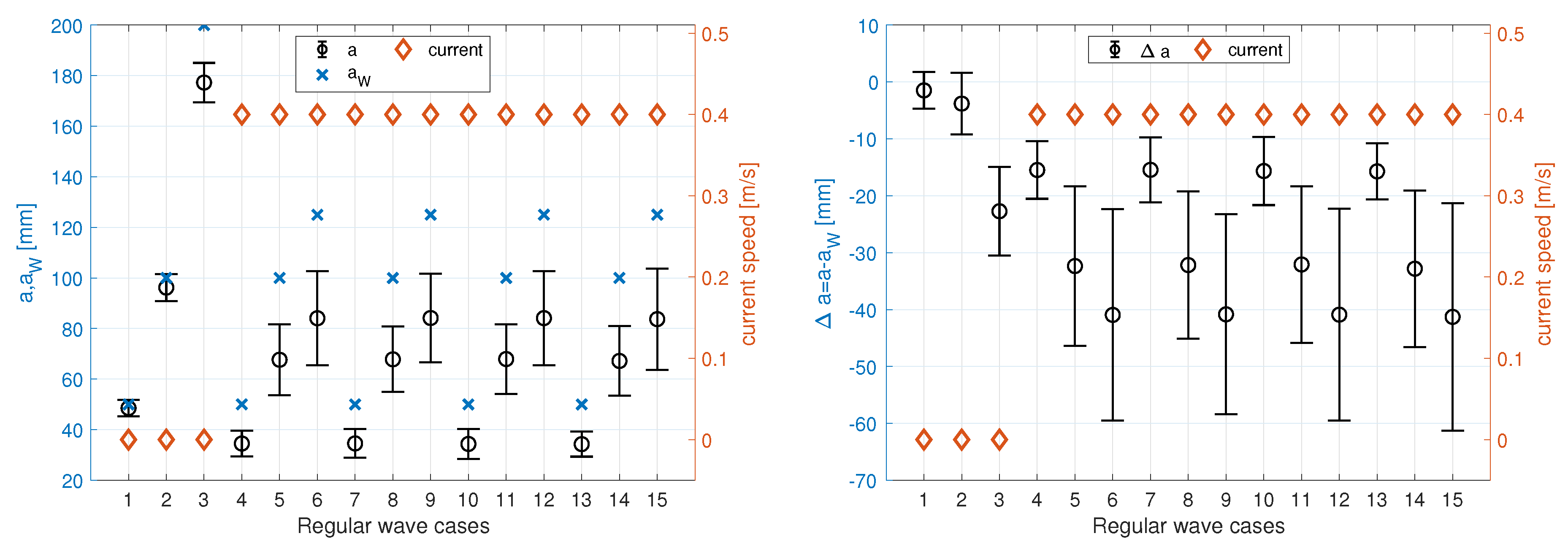
Three different regular waves were investigated with a constant wave frequency $f_W$ of 0.5 Hz. Table 3 presents an overview of the chosen input values. Initially also a wave amplitude of 0.2 m was investigated for the 0 m/s flow speed, which was for the further tests reduced to 0.125 m. Wave cases Reg4 to Reg15 provide three similar waves for a following flow speed of 0.4 m/s. Those cases include three different obstacle distances as well as the ROV only configuration.

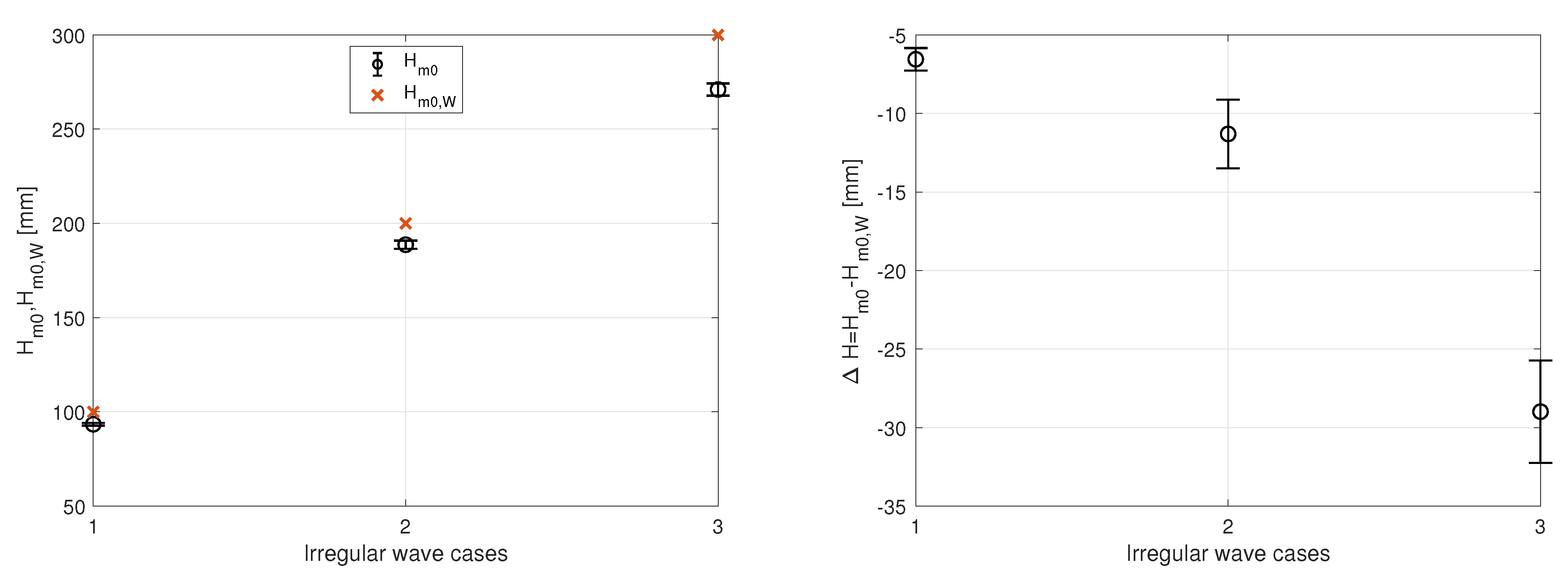
Irregular waves were only investigated in absence of currents. Three different heights $H_{m0,W}$ were defined and a constant random value (seed) 3.0 [-] was used. All the other parameters are shown in Table 4. Both regular and irregular waves are only exemplary and should allow to help to quantify the effect of the wave load on the ROV.

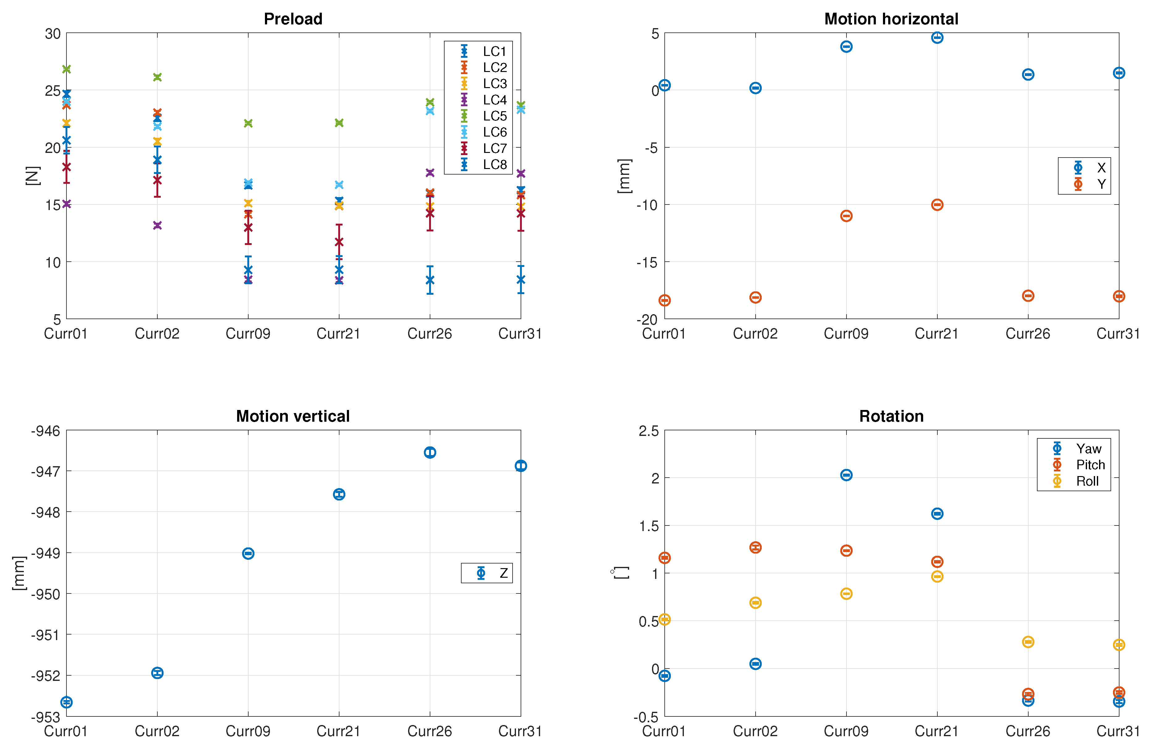
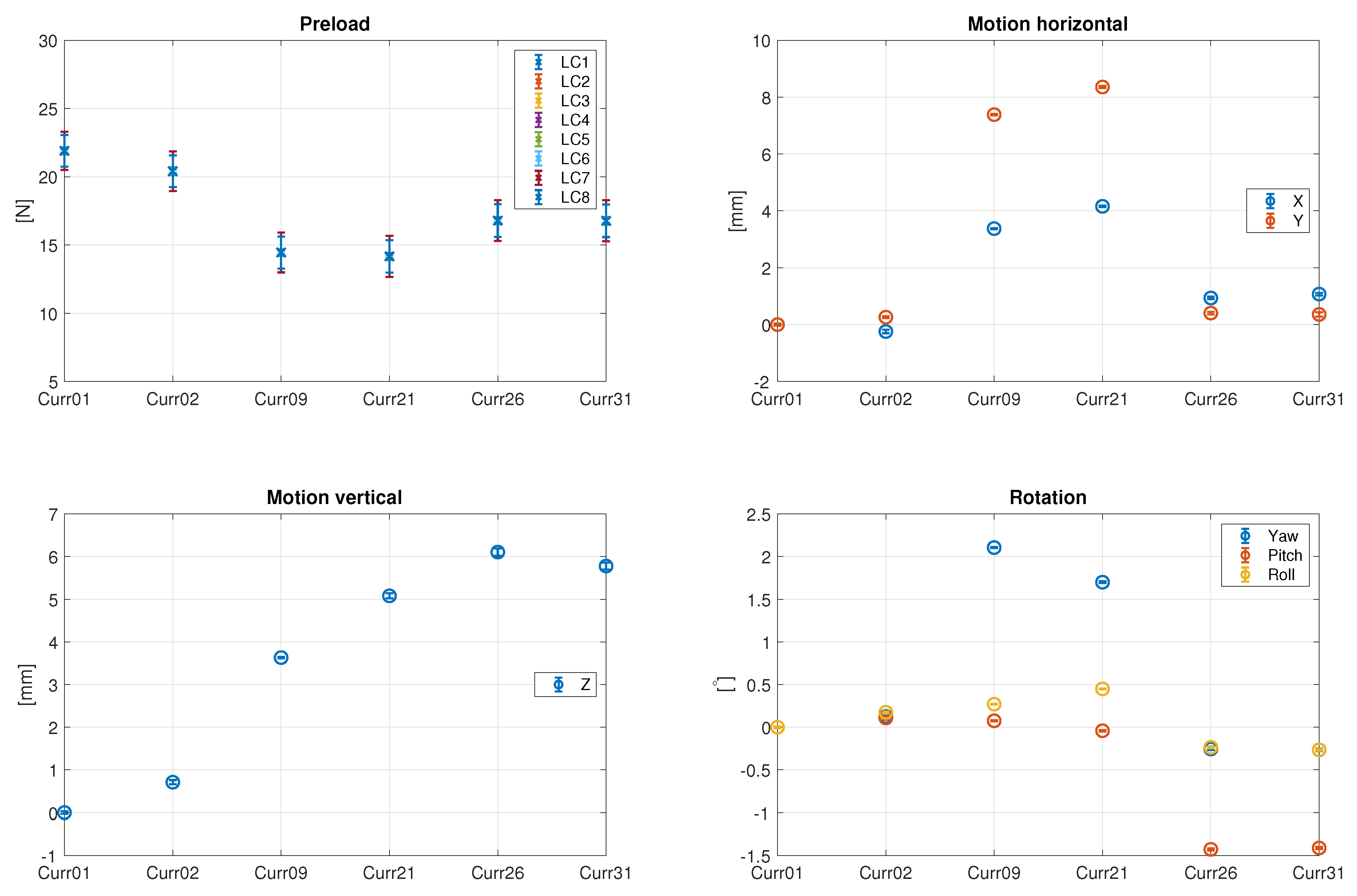
Table 5 presents an overview of investigated cases for which the ROV was active and provided thrust and forces into the tethers. Two still cases allow a quantification of the preload in each tether for the fully submerged case. Those cases are identical to the Curr01 and Curr02 in Table 6. During the first eight measurements the ROV received a steady state command and after a stabilisation period the capturing of data was triggered. During the second group of measurements, the ROV moved dynamically in one main direction. For the sake of completeness, it has to be mentioned that no obstacle was present for those tests.

Table 6 presents the cases, which were characterised by pure flow conditions in different directions and speeds, with and without the obstacle at three different distances. The speed of the flow varies from 0 m/s up to 1 m/s in the centre of the tank. The measurements with the highest velocities, namely Curr07 and Curr08, mobilised a big amount of seeding (neutral buoyant glass spheres), which reduced the visibility in the tank. The seeding was added to the water during previous experimental investigations to measure the flow speed. The light settings for the MoCAP were constantly monitored and corrected, but in some cases the changes were too big and data could not be provided for the full length of the tests. The previously mentioned two cases as well as the run Curr20 includes substantial missing data, which is represented as NaNs (Not a Number) in the file. The other files also include very rare occasions when this happened. Nevertheless, the length of the tests should provide good data for the steady conditions.

With an obstacle placed in front of the ROV the velocity was initially limited to 0.6 m/s, but the construction proved to be very stable. Hence, the control case of flow from the back (Curr22, flow direction 0${}^{°}$) was replaced by an additional increased velocity of 0.8 m/s for the closest and middle distance of the cylinder to the ROV.

3. Additional Analysis

The following section contains additional analysis of the provided data, which are not part of the paper [3]. It includes the analysis of the WG data as well as the comparison of the preloads over the investigation period including the splitting into the main directions for the forces.

3.1. Wave Gauges

In a first step, the measured waves are compared to the requested values from the wave makers. The wave frequency was for all cases exactly 0.5 Hz. The wave heights were lower then requested. This is well know for the currently used transfer function in FloWave [30] and can be corrected by increasing the input amplitude. This effect is even more enhanced for following waves by adding current. Figure 2 presents the requested wave amplitude $a_W$ as well as the measured value a based on a FFT analysis as well as the difference $\Delta a$ between the two. The error bar shows the spread from the mean value to the maximum value of the six WG and the values are provided in Table 3. Similar investigations were conducted for the three irregular waves and presented in Figure 3 and

Table 7. Comparison requested amplitude $a_W$ and wave height $H_s$ to the measured values a for regular and $H_{m0}$ for irregular waves (definition presented in Table 3 and Table 4; visualisation Figure 2 and Figure 3).

Number	Amp ${\mathit{a}}_{\mathit{W}}$	Amp a	$\mathit{a}/{\mathit{a}}_{\mathit{W}}$		Number	Amp ${\mathit{a}}_{\mathit{w}}$	Amp a	$\mathit{a}/{\mathit{a}}_{\mathit{W}}$
	[mm]	[mm]	[%]			[mm]	[mm]	[%]
Reg01	50	48.52	97.0%		Reg11	100	67.92	67.9%
Reg02	100	96.19	96.2%		Reg12	125	84.11	67.3%
Reg03	200	177.28	88.6%		Reg13	50	34.29	68.6%
Reg04	50	34.52	69.0%		Reg14	100	67.18	67.2%
Reg05	100	67.65	67.7%		Reg15	125	83.71	67.0%
Reg06	125	84.06	67.3%
Reg07	50	34.56	69.1%		Number	$H_{m0,W}$$\left[\mathrm{mm}\right]$	$H_{m0}$$\left[\mathrm{mm}\right]$	$H_{m0}/H_{m0,W}$$[\%]$
Reg08	100	67.82	67.8%		Irr01	100	93.45	93.4%
Reg09	125	84.16	67.3%		Irr02	200	188.69	94.3%
Reg10	50	34.35	68.7%		Irr03	300	271.01	90.3%

. All waves were following the current flow direction (where current was present).

3.2. Load Cells

The installation of the ROV was conducted in the dry upon the raised tank floor. In the dry condition the full weight of the ROV was supported by the upper tethers from LC5 to LC8.

The target was not to overload the upper load cells (LC) with preloads of the lower LCs and to position the ROV in the mid water depth over the tank centre. In the submerged condition, the four lower LC have a higher hydro-static pressure than the upper ones and the additional buoyancy of the ROV resulted in an upward force (negative z-direction) in the range of 4.2 N. The individual preload could only be corrected with a raised floor. An aim of the installation was to ensure a homogeneous value of all eight LC in the range of 20 N but a sufficient minimum value was accepted. It was assumed that that all previous mentioned effects, namely hydro-static difference, preload and buoyancy, were constant. The further analysis, presented in Gabl et al. [3], focus on the additional hydrodynamic forces due to current and waves.

To identify the constant forces, six still water (zero) measurements were conducted distributed over the full testing program. Figure 4 presents the results of the steady state measurements of the LC without a flow speed and also shows the average values of the motion capturing system. The error bars represent the standard deviation over the individual full capture time. Obviously, LC7 and LC8 had an increased rated capacity of 500 N and were comparably noisy under these low forces. A potential solution would be to add a 16 Hz low pass filter to improve the signal quality. The other LC with a rated capacity of 100 N have a significantly smaller standard deviation. The decrease of the measured value in all LCs from the zero measurement Curr02 to the following Curr09 (Figure 4) could be cased by a drift of the LC but more likely by a change in the length of one or more tethers. This is indicated by changes in the location and orientation of the ROV. It has to be mentioned that high velocities were tested between those two cases as well as further activation of the ROV (not part of this published dataset). To prevent a further reduction of the pre-tension, it was increased in the lower tethers, which brought the model back to the initial position.

Correction values for the other tests were calculated based on these six zero measurements. As mentioned previously, it is assumed that the forces in all tethers should be equal. Hence, an individual correction value for each LC and zero measurement was calculated to present equal values with the same average value. Figure 5 presents the corrected values for the zero measurement. The similar corrections were applied for the further measurements.

Table 8. Used corrections values for the provided cases; correction value C identify which of the six conducted zero measurements was used, for example, if C = 1, the Curr01 is used and so on up to C = 6 for Curr31.

Number	C	Number	C	Number	C	Number	C	Number	C	Number	C
Curr01	1	Curr13	3	Curr25	4	Mot01	1	Mot13	2	Reg07	4
Curr02	2	Curr14	3	Curr26	5	Mot02	1	Mot14	2	Reg08	4
Curr03	2	Curr15	3	Curr27	5	Mot03	1	Mot15	2	Reg09	4
Curr04	2	Curr16	3	Curr28	5	Mot04	1	Mot16	2	Reg10	5
Curr05	2	Curr17	3	Curr29	5	Mot05	1	Mot17	2	Reg11	5
Curr06	2	Curr18	3	Curr30	5	Mot06	1	Mot18	2	Reg12	5
Curr07	2	Curr19	3	Curr31	6	Mot07	1	Reg01	3	Reg13	6
Curr08	2	Curr20	3	Curr32	6	Mot08	1	Reg02	3	Reg14	6
Curr09	3	Curr21	4	Curr33	6	Mot09	1	Reg03	3	Reg15	6
Curr10	3	Curr22	4	Curr34	6	Mot10	2	Reg04	3	Irr01	3
Curr11	3	Curr23	4	Curr35	6	Mot11	2	Reg05	3	Irr02	3
Curr12	3	Curr24	4			Mot12	2	Reg06	3	Irr03	3

documents the connection between the number and the applied correction case. In contrast to the LC, the motion capturing results are only corrected by the first measurement (Curr01). Consequently, the further presented motions and rotations are relative changes to the initial position. As mentioned in Section 4, the initial measured values as well as the processed values are provided.

In a second step, the measured value F of the LC are split into the main directions $F_x,F_y$ and $F_z$ according to the vector $\overrightarrow{V}=[V_x,V_y,V_z]$, which was calculate based Equation (1). This processing was done for each of the LC based on the definition shown in Figure 6. The steps are described in the following equations:

$$\begin{array}{c}\hfill F_z=F·sin\left(\alpha \right);F_{xy}=F·cos\left(\alpha \right)\ast dir\left(i\right);F_x=F_{xy}·cos\left(\beta \right);F_y=F_{xy}·sin\left(\beta \right)\end{array}$$

(2)

$$\begin{array}{c}\hfill V_{xy}={\left(V_x^2+V_y^2\right)}^{0.5};\alpha =arctan(V_z/V_{xy});\beta =arctan(V_y/V_x);dir=[1,1,-1,-1,1,1,-1,-1]\end{array}$$

(3)

All LC provided a positive value but four of the eight LC faced in a different direction (Figure 1). Consequently, a correction vector $dir$ had to be introduced to ensure the correct direction of the horizontal forces. The i subscript represents the number of the LC. The influence of the previously mentioned correction of the LC on the forces in the main direction can be seen by comparing the Figure 7 and Figure 8. Each one presents a summary of the total sum in each direction as well as a detailed view of each direction, which includes the positive and negative (multiplied by −1) subtotals. As shown in Figure 8, after the correction the total sum of forces for the zero measurements are in a very small range of ±1 N.

4. Dataset Description

In total 178 txt-files are provided via the DataShare of the University of Edinburgh [4]. It is split in two different types of data: (a) Raw data (RD), which includes the measured values, and (b) processed data (PD). For the latter the load cell (LC) data is corrected and split into the main directions for each mounting point as presented in Section 3.2. The name of each file starts either with RD or PD to indicate the different processing states and further includes the case identification (ID) as well as the run ID starting with 01:

RD or PD_ [case ID] [run ID] _CaptureTime.txt

RD_ or PD_ [case ID] [run ID] _RepeatTime.txt (only for wave cases)

The inputs for the cases with the ID Reg are summarised in Table 3, Irr in Table 4, Mot in Table 5 and the current only cases, Curr, in Table 6. For all cases the full capture time is provided. An additional file with the changed suffix (_RepeatTime) is added for the test that include waves. For both cases, namely capture and repeat time, those files include the wave gauge data of WG1 to WG6.

The header for the raw data is provided in

Table 9. Raw data; content of the files for each individual case; ${}^{*}$ wave gauge (WG) data is only added for the regular and irregular waves case, which also includes an additional file for the repeat time.

Name	Time	X	Y	Z	yaw	pitch	roll		⋯
Unit	[sec]	[mm]	[mm]	[mm]	[°]	[°]	[°]		⋯
Column	1	2	3	4	5	6	7		⋯
	LC1	LC2	LC3	LC4	LC5	LC6	LC7	LC8	⋯
	[N]	[N]	[N]	[N]	[N]	[N]	[N]	[N]	⋯
	8	9	10	11	12	13	14	15	⋯
	$V_{xLC1}$	$V_{yLC1}$	$V_{zLC1}$	⋯	$V_{xLC8}$	$V_{yLC8}$	$V_{zLC8}$		⋯
	[mm]	[mm]	[mm]	⋯	[mm]	[mm]	[mm]		⋯
	16	17	18	⋯	37	38	39		⋯
	WG1 ${}^{*}$	WG2 ${}^{*}$	WG3 ${}^{*}$	WG4 ${}^{*}$	WG5 ${}^{*}$	WG6 ${}^{*}$
	[mm]	[mm]	[mm]	[mm]	[mm]	[mm]
	40	41	42	43	44	45

and

Table 10. Processed data; content of the files for each individual case; ${}^{*}$ wave gauge (WG) data is only added for the regular and irregular waves case, which also includes an additional file for the repeat time.

Name	time	X	Y	Z	yaw	pitch	roll	⋯
Unit	[sec]	[mm]	[mm]	[mm]	[°]	[°]	[°]	⋯
Column	1	2	3	4	5	6	7	⋯
	$F_{xLC1}$	⋯	$F_{xLC8}$	$F_{yLC1}$	⋯	$F_{yLC8}$	$F_{zLC1}$	⋯	$F_{zLC8}$	⋯
	[N]	⋯	[N]	[N]	⋯	[N]	[N]	⋯	[N]	⋯
	8	⋯	15	16	⋯	23	24	⋯	31	⋯
	WG1 ${}^{*}$	WG2 ${}^{*}$	WG3 ${}^{*}$	WG4 ${}^{*}$	WG5 ${}^{*}$	WG6 ${}^{*}$
	[mm]	[mm]	[mm]	[mm]	[mm]	[mm]
	32	33	34	35	36	37

presents the similar information for the processed data. The first column includes a time vector based on the measurement frequency of 128 Hz. X, Y and Z are the motions in the coordinate directions. The definition for yaw, pitch and roll is provided in Figure 6. In the processed data those values are relative to the mean value of the first measurements. The eight load cell (LC) values and tether vectors ($V_{xLCi}$, $V_{yLCi}$, $V_{zLCi}$) are the input values for the split of the forces into the main coordinate direction ($F_{xLCi}$, $F_{yLCi}$, $F_{zLCi}$). Details are presented in Section 3.2.

References

1. Hastie, H.; Lohan, K.; Chantler, M.; Robb, D.A.; Ramamoorthy, S.; Petrick, R.; Vijayakumar, S.; Lane, D. The ORCA Hub: Explainable Offshore Robotics through Intelligent Interfaces. In Proceedings of the 13th Annual ACM/IEEE International Conference on Human Robot Interaction, Chicago, IL, USA, 5–8 March 2018. [Google Scholar]
2. Sayed, M.E.; Nemitz, M.P.; Aracri, S.; McConnell, A.C.; McKenzie, R.M.; Stokes, A.A. The Limpet: A ROS-Enabled Multi-Sensing Platform for the ORCA Hub. Sensors 2018, 18, 3487. [Google Scholar] [CrossRef] [Green Version]
3. Gabl, R.; Davey, T.; Cao, Y.; Li, Q.; Li, B.; Walker, K.L.; Giorgio-Serchi, F.; Aracri, S.; Kiprakis, A.; Stokes, A.; et al. Hydrodynamic Loads on a Restrained ROV under Waves and Current. 2020; submitted. [Google Scholar]
4. Gabl, R.; Davey, T.; Cao, Y.; Li, Q.; Li, B.; Walker, K.L.; Giorgio-Serchi, F.; Aracri, S.; Kiprakis, A.; Stokes, A.A.; et al. Dataset—Experimental Force Data of a Restrained ROV under Waves and Current; Edinburgh DataShare [Dataset]; University of Edinburgh: Edinburgh, UK, 2020. [Google Scholar] [CrossRef]
5. Selvakumar, J.M.; Asokan, T. A Novel Approach to Measure under Water Vehicle Disturbance Force for Station Keeping Control. In Proceedings of the 9th International Conference on Informatics in Control, Automation and Robotics, Rome, Italy, 28–31 July 2012; Volume 2, pp. 460–463. [Google Scholar]
6. Wang, W.; Clark, C.M. Modeling and Simulation of the VideoRay Pro III Underwater Vehicle. In Proceedings of the OCEANS 2006—Asia Pacific, Singapore, 16–19 May 2006; pp. 1–7. [Google Scholar]
7. Inoue, T.; Suzuki, H.; Shimamura, T.; Nakajima, K.; Shioji, G. Experimental research on horizontal rotation of ROV induced by external forces near sea surface. In Proceedings of the OCEANS 2008, Quebec City, QC, Canada, 15–18 September 2008; pp. 1–6. [Google Scholar]
8. Eng, Y.H.; Lau, W.S.; Low, E.; Seet, G.; Chin, C.S. Estimation of the Hydrodynamics Coefficients of an ROV using Free Decay Pendulum Motion. Eng. Lett. 2008, 16, 326–331. [Google Scholar]
9. Morrison, A.T.; Yoerger, D.R. Determination of the hydrodynamic parameters of an underwater vehicle during small scale, nonuniform, 1-dimensional translation. In Proceedings of the OCEANS ’93, Victoria, BC, Canada, 18–21 October 1993; Volume 2, pp. II277–II282. [Google Scholar]
10. Lack, S.; Rentzow, E.; Jeinsch, T. Experimental Parameter Identification for an open-frame ROV: Comparison of towing tank tests and open water self-propelled tests. IFAC-PapersOnLine 2019, 52, 271–276. [Google Scholar] [CrossRef]
11. Roy, P.D.; Ranjan, R. Variation of Wave Force on Submerged Object at Shallow Water: Fourier Series Technique. Aquatic Procedia 2015, 4, 95–102. [Google Scholar] [CrossRef]
12. Roy, P.D.; Ghosh, S. Wave force on vertically submerged circular thin plate in shallow water. Ocean Eng. 2006, 33, 1935–1953. [Google Scholar] [CrossRef]
13. Sakiyama, J.; Motoi, N. Position and Attitude Control Method Using Disturbance Observer for Station Keeping in Underwater Vehicle. In Proceedings of the IECON 2018—44th Annual Conference of the IEEE Industrial Electronics Society, Washington, DC, USA, 21–23 October 2018; pp. 5469–5474. [Google Scholar] [CrossRef]
14. Willy, C.J. Attitude Control of an Underwater Vehicle Subjected to Waves. Master’s Thesis, MIT and Woods Hole Oceanographic Institution, Cambridge, MA, USA, 1994. [Google Scholar]
15. Milgram, J.H. Strip theory for underwater vehicles in water of finite depth. J. Eng. Math. 2007, 58, 31–50. [Google Scholar] [CrossRef] [Green Version]
16. Yang, R.; Clement, B.; Mansour, A.; Li, M.; Wu, N. Modeling of a Complex-Shaped Underwater Vehicle for Robust Control Scheme. J. Intell. Robot. Syst. 2015, 80, 491–506. [Google Scholar] [CrossRef]
17. Singh, Y.; Bhattacharyya, S.K.; Idichandy, V.G. CFD approach to modelling, hydrodynamic analysis and motion characteristics of a laboratory underwater glider with experimental results. J. Ocean Eng. Sci. 2017, 2, 90–119. [Google Scholar] [CrossRef]
18. Dukan, F.; Ludvigsen, M.; Sørensen, A.J. Dynamic positioning system for a small size ROV with experimental results. In Proceedings of the IEEE OCEANS 2011, Santander, Spain, 6–9 June 2011; pp. 1–10. [Google Scholar]
19. Ingram, D.; Wallace, R.; Robinson, A.; Bryden, I. The Design and Commissioning of the First, Circular, Combined Current and Wave Test Basin. In Proceedings of the IEEE Oceans 2014 MTS/IEEE, Taipei, Taiwan, 7–10 April 2014. [Google Scholar]
20. Draycott, S.; Sellar, B.; Davey, T.; Noble, D.R.; Venugopal, V.; Ingram, D. Capture and Simulation of the Ocean Environment for Offshore Renewable Energy. Renew. Sustain. Energy Rev. 2019, 104, 15–29. [Google Scholar] [CrossRef]
21. Walker, K.L.; Stokes, A.A.; Kiprakis, A.; Giorgio-Serchi, F. Impact of Thruster Dynamics on the Feasibility of ROV Station Keeping in Waves. In Proceedings of the OCEANS 2020 MTS/IEEE, Singapore, 5–30 October 2020. in press. [Google Scholar]
22. Walker, K.L.; Stokes, A.A.; Kiprakis, A.; Giorgio-Serchi, F. Investigating PID Control for Station Keeping ROVs. In Proceedings of the UKRAS20 Conference: “Robots into the real world”, Lincoln, UK, 17 April 2020; pp. 51–53. [Google Scholar]
23. Blue Robotics, “BlueROV2” Datasheet, June 2016 [Revised Jan. 2019]. Available online: https://bluerobotics.com/wp-content/uploads/2020/02/br_bluerov2_datasheet_rev6.pdf (accessed on 2 June 2020).
24. NVIDIA Jetson Nano Developer Kit. Available online: https://www.nvidia.com/en-gb/autonomous-machines/embedded-systems/jetson-nano/ (accessed on 2 June 2020).
25. Blue Robtotics, Ping360 Scanning Imaging Sonar. Available online: https://bluerobotics.com/store/sensors-sonars-cameras/sonar/ping360-sonar-r1-rp/ (accessed on 2 June 2020).
26. APPLIED MEASUREMENTS Ltd. Submersible Load Cell–DDEN. Available online: https://appmeas.co.uk/products/load-cells-force-sensors/in-line-submersible-load-cell-dden/ (accessed on 2 June 2020).
27. MARINET (2012). Work Package 2: Standards and Best Practice—D2.1 Wave Instrumentation Database. Revision: 05. Available online: http://www.marinet2.eu/wp-content/uploads/2017/04/D2.01-Wave-Instrumentation-Database.pdf (accessed on 2 June 2020).
28. Gabl, R.; Steynor, J.; Forehand, D.I.M.; Davey, T.; Bruce, T.; Ingram, D.M. Capturing the Motion of the Free Surface of a Fluid Stored within a Floating Structure. Water 2019, 11, 50. [Google Scholar] [CrossRef] [Green Version]
29. Noble, D.; Davey, T.; Smith, H.; Panagiotis, K.; Robinson, A.; Bruce, T. Spatial variation of currents generated in the FloWave Ocean Energy Research Facility. In Proceedings of the 11th European Wave and Tidal Energy Conference (EWTEC2015), Nantes, France, 6–11 September 2015. [Google Scholar]
30. Gabl, R.; Davey, T.; Nixon, E.; Steynor, J.; Ingram, D.M. Experimental Data of a Floating Cylinder in a Wave Tank: Comparison Solid and Water Ballast. Data 2019, 4, 146. [Google Scholar] [CrossRef] [Green Version]
Figure 1. Experimental set-up with the restrained ROV on the raised tank floor including numbered load cells (a); submerged conditions including the wave gauges (WG) (b). The blue arrow indicates the main direction of the generated waves and current at 180 ° .
Data 05 00057 g001
Figure 2. Analysis WG regular waves; comparison of the requested wave amplitude a W to the measured value a; difference compared with the current speed; the error bar indicates the range of the five WGs in relation to the average.
Data 05 00057 g002
Figure 3. Analysis WG irregular waves; comparison of the requested wave height H m 0 , W to the measured value H m 0 ; the error bar indicates the range of the five WGs to the average.
Data 05 00057 g003
Figure 4. Analysis of the still water measurements; load cell (LC) values, motion and rotation; initial measurements.
Data 05 00057 g004
Figure 5. Analysis of the still water measurements; LC values, motion and rotation; corrected values.
Data 05 00057 g005
Figure 6. Sketch for the splitting of the forces into the main directions; definition of the rotations roll, pitch and yaw.
Data 05 00057 g006
Figure 7. Analysis of the still water measurements; summary and detailed view of the forces in the main directions; initial measurements.
Data 05 00057 g007
Figure 8. Analysis of the still water measurements; summary and detailed view of the forces in the main directions; corrected values.
Data 05 00057 g008