
SEN2VENµS, a Dataset for the Training of Sentinel-2 Super-Resolution Algorithms


CESBIO, Université de Toulouse, CNES, CNRS, INRAE, IRD, UT3, 18 Avenue Edouard Belin BPI 2801, CEDEX 9, 31401 Toulouse, France
*
Author to whom correspondence should be addressed.
Data 2022, 7(7), 96; https://0-doi-org.brum.beds.ac.uk/10.3390/data7070096
Submission received: 13 May 2022
/
Revised: 4 July 2022
/
Accepted: 11 July 2022
/
Published: 13 July 2022
/
Corrected: 28 February 2023
(This article belongs to the Section Spatial Data Science and Digital Earth)
Abstract
:Boosted by the progress in deep learning, Single Image Super-Resolution (SISR) has gained a lot of interest in the remote sensing community, who sees it as an opportunity to compensate for satellites’ ever-limited spatial resolution with respect to end users’ needs. This is especially true for Sentinel-2 because of its unique combination of resolution, revisit time, global coverage and free and open data policy. While there has been a great amount of work on network architectures in recent years, deep-learning-based SISR in remote sensing is still limited by the availability of the large training sets it requires. The lack of publicly available large datasets with the required variability in terms of landscapes and seasons pushes researchers to simulate their own datasets by means of downsampling. This may impair the applicability of the trained model on real-world data at the target input resolution. This paper presents SEN2VENµS, an open-data licensed dataset composed of 10 m and 20 m cloud-free surface reflectance patches from Sentinel-2, with their reference spatially registered surface reflectance patches at 5 m resolution acquired on the same day by the VENµS satellite. This dataset covers 29 locations on earth with a total of 132,955 patches of 256 × 256 pixels at 5 m resolution and can be used for the training and comparison of super-resolution algorithms to bring the spatial resolution of 8 of the Sentinel-2 bands up to 5 m.
Data Set: https://zenodo.org/record/6514159.
Data Set License: Etalab Open Licence Version 2.0, Creative Commons BY-NC 4.0, Creative Commons BY 4.0.
1. Introduction
Among the global coverage and free and open-data policy earth observation missions in the optical domain, Sentinel-2 is currently the one with the highest spatial resolution. There is currently no open alternative to Sentinel-2 10 m imagery with 5 days revisit on a global or even a regional scale, and most probably there will not be any until the launch of the next generation of Sentinel-2 satellites. A resolution of 10 m can be limiting for some applications, and thus the promise of Single Image Super-Resolution (SISR), which claims to offer a significant increase in resolution without any additional input but the 10 m Sentinel-2 image itself, has raised a lot of interest in the remote sensing community.
Remote sensing satellites often offer several spectral bands with different resolutions for a given sensor. For instance, Sentinel-2 has 10 m resolution blue, green, red and wide near infrared channels but three red edge bands and a narrow infrared channel at 20 m resolution and atmospheric correction bands at 60 m resolution. In the literature, there are several model-based methods aimed at sharpening all bands to the highest sensor resolution [1,2,3], as well as deep-learning-based methods [4,5,6,7,8]. Though this demonstrates a clear interest for improving the spatial resolution of existing sensors in remote sensing, those algorithms differ from SISR by the fact that the target resolution is limited to the highest resolution among bands (e.g., 10 m for Sentinel-2), whereas SISR targets resolutions higher than the highest band’s resolution (e.g., higher than 10 m for Sentinel-2).
Single Image Super-Resolution is the task of obtaining a higher resolution version of a single image, using no other inputs that the image itself. In the context of remote sensing satellite imagery, higher resolution means that not only the same area on the ground is covered by a higher number of smaller pixels, which can be achieved by means of traditional spatial re-sampling techniques, but also that the super-resolved image exhibits faithful higher spatial frequency content with respect to the original image.
Super-resolution is an ill-posed inverse problem, as many higher resolution predictions can explain the same low-resolution image. Prior to the deep learning era, super-resolution was considered as a blind deconvolution problem. It has therefore been traditionally tackled by regularization constraints during optimization to promote desired properties of the prediction, such as piece-wise smoothness, with total variation [9], or sparsity [10].
The advent of deep learning gave a fresh start to the Single Image Super-Resolution problem, for which convolutional, residual and then generative–adversarial architectures have been proposed with success [11,12]. Provided that enough data are available for training, it is possible to estimate a nonlinear mapping with a few hundred thousand parameters that undoes all the high frequency damping and aliasing occurring at sensor level, and even generates plausible high resolution details past the cut-off frequency of the sensor. To feed those data-hungry algorithms and lay grounds for architecture contests, several natural images datasets have been published [13,14,15]. Most of these datasets are put up by downsampling the high resolution image, using the original high resolution image as a reference for training, validation and testing. In practice, this simulation of the low resolution data leads to a simplified version of the problem by ignoring parameters of low resolution acquisition, such as noise or compression artifacts. This, in turn, may lead to lesser performances when applied to real world data.
Remote sensing images are very different in nature from natural images used in the previously cited natural images datasets: the image content itself is different, consisting in Earth surface observed from an almost fixed altitude, which means objects of typical sizes will always be represented by roughly the same amount of pixels. More importantly, remote sensing images can capture earth radiance in several wavelength bands that may or may not include what is called red, green and blue in natural images, with a bit depth exceeding the traditional 8-bits encountered in most natural images. Moreover, spectral bands may be acquired at different spatial resolutions. There is therefore a need for a dedicated dataset that can represent all the specifics of remote sensing imagery in the development and comparison of super-resolution algorithms.
The progress of Single Image Super-Resolution of course raised a lot of interest in the field of remote sensing optical imagery [16] and its never-ending race for better resolution. In [17], the authors train a CNN to super-resolve Landsat images by using Sentinel-2 as the target. In [18], the authors use nine RapidEye images at 5 m resolution as a target to train a Sentinel-2 super-resolution EDSR network. More recent work includes [19] in which the authors train the ESRGAN network with Sentinel-2 images as input and 32 Worldview-2/3 images over European cities at 2 m resolution as target, thus achieving a factor of five in spatial resolution. In [20], the authors train the SRGAN network with Sentinel-2 images as input and 41 PeruSat-1 images over Peru at 2.8 m resolution as target. In [21], the authors propose the TARSGAN network, which is trained with data simulated from 102 Deimos-2 images at 1 m resolution and then apply the method to super-resolve Sentinel-2 images. In [22], the author trained a modified EDSR network with 12 pairs of Sentinel-2 and PlanetScope images, for a target resolution of 2.5 m to 5 m.
If the results presented in those works are promising, they are using very limited datasets in terms of landscape and season variability, which can be explained by the scarcity of available very high resolution commercial imagery for research. Most importantly, none of those datasets has been made publicly available to allow the scientific community members to reproduce and challenge those results and improve their own methods. In fact, to the best of our knowledge, no remote sensing Single Image Super-Resolution dataset has been made publicly available yet. There is, however, a public dataset dedicated to the super-resolution of Proba-V images using multiple images (Multiple Images Super-Resolution) [23].
This paper does not propose any new SIRS method, nor is it benchmarking existing SISR methods. Instead, the aim of this paper is to describe the source data, generation process and content of SEN2VENµS, an open dataset for the super-resolution of Sentinel-2 images built by leveraging simultaneous acquisitions with the VENµS satellite (see Section 2.1 for a detailed description of those satellite missions). This dataset has been made publicly available in hopes to laying the groundwork for future work in the remote sensing community for fair benchmarking, comparison and further research on SISR methods, using data that are representative of remote sensing usages. The dataset is composed of 10 m and 20 m cloud-free surface reflectance patches from Sentinel-2, with their reference spatially registered surface reflectance patches at 5 m resolution acquired on the same day and within 30 min at most by the VENµS satellite. It covers 29 locations with a total of 132,955 patches of 256 × 256 pixels at 5 m resolution. It can be used for the training and comparison of super-resolution algorithms to bring spatial resolution of eight of the Sentinel-2 bands up to 5 m.
2. Dataset Generation
2.1. Sentinel-2 and VENµS Missions
Sentinel-2 is the well known high revisit optical Copernicus mission operating since mid-2015 [24]. It provides full coverage of all lands between 56° south and 84° north, every 5 days at most, in 13 spectral bands in 3 different resolution groups: 10 m for visible bands and wide near infrared (NIR), 20 m for red edges bands and narrow NIR and 60 m for coastal blue and atmospheric corrections bands. Viewing angles from a given orbit are constant and lower than 12°, and the orbit crosses the equator at 10h30 local time. Sentinel-2 data are distributed with an open-data policy, and recurring satellites are provisioned until 2035. Sentinel-2 is therefore a major stable source for remote sensing optical imagery and widely used in many applications [25,26,27].
Vegetation and environment monitoring on a New Micro-Satellite (VENµS) is a French–Israeli satellite providing a very high revisiting frequency of 2 days on a selection of 125 sites around the world, with constant viewing angles since 2017 [28,29]. VENµS provides 5 m observations in 12 spectral bands, among which traditional visible bands, red edge and near infrared bands closely match Sentinel-2 spectral bands, as shown in Figure 1. Note that despite its very large bandwidth that does not really match any band in VENµS, the Sentinel-2 B8 band has been kept, since it is the only near infrared domain Sentinel-2 band sampled at 10 m resolution.
2.2. Product Levels and Processing
Remote sensing imagery products come in different levels depending on the applied processing. End users usually work with products of at least level 2A, which includes, among other things:
- Ortho-rectification (geometric processing);
- Atmospheric correction: Conversion of radiance to surface reflectance values, including estimation and compensation of aerosol content and water vapor amount;
- Screening of clouds and cloud shadows.
Though ESA delivers L2A products from their own processor Sen2Corr, L2A products generated by the MAJA open-source processing chain developed by CNES and CESBIO [30] have been used in this work. The rationale behind this is that both VENµS archive and a subset of the Sentinel-2 archive is produced by CNES at level 2A with MAJA and distributed on the Theia portal (https://theia.cnes.fr) (accessed on 12 May 2022). Therefore, VENµS and Sentinel-2 images used in the proposed dataset were produced by the exact same algorithms and code, which enforces the coherence between both products. Table 1 summarizes the corresponding spectral bands between Sentinel-2 and VENµS that are sampled in the SEN2VENµS dataset. For both sensors, surface reflectance with adjacency effect compensation has been used.
Both sensors offer the same range of validity flags, namely:
- A mask of no-data pixels, which are out of the sensor swath;
- A mask of clouds and clouds shadows;
- A mask of saturated pixels;
- A mask of geophysically invalid pixels (water, out of sight pixels due to relief, etc…).
From all those masks, a single validity mask is derived for each product by taking their union.
Sentinel-2 L2A products distributed by Theia are subject to the Etalab Open Licence Version 2.0 (https://theia.cnes.fr/atdistrib/documents/Licence-Theia-CNES-Sentinel-ETALAB-v2.0-en.pdf) (accessed on 12 May 2022). VENµS L2A products distributed by Theia are subject to the Creative Commons BY-NC 4.0 (https://creativecommons.org/licenses/by-nc/4.0/) (accessed on 12 May 2022).
2.3. Site Selection
Figure 2 shows the available VENµS sites as well as the Sentinel-2 coverage available on Theia. One can see that many VENµS sites are not covered by available Sentinel-2 tiles, for instance in North America, Australia and Japan. Among the covered VENµS sites, 29 sites have been selected based on the amount of same day co-ocurrences, represented by red dots in Figure 2. Note that since there are many more VENµS sites available, the dataset can always be extended by producing the corresponding Sentinel-2 tiles to level 2A with the MAJA processor. It would of course also be possible to use Sen2Cor L2A products distributed on Scihub (https://scihub.copernicus.eu/) (accessed on 12 May 2022), at the expense of less consistency due to the use of different L2A processing chains between VENµS and Sentinel-2. Each site is identified by a unique name for which country, province name and center location are summarized in Table 2. One can observe than more than half of the sites are located in Europe, and that nine sites are located in tropical areas. The swath of the VENµS instrument is 27.8 km, and most sites correspond roughly to a square area.
To show the variability of this selection of sites with respect to land cover, Figure 3 shows the proportions of land-cover classes from the Copernicus 2019 Land-Cover map [31] within each selected Venµs site. In total, half of the covered area contains forests, one-third contains croplands and 5% correspond to built-up areas. These proportions vary greatly depending on the site, with sites in South America being almost fully covered by forests, while others in Europe, North America and India are mostly covered by croplands. Urban areas account for up to 15% at most, and the Kyrgyzstan site is almost fully covered with herbaceous vegetation.
It is important to note that if the viewing angles of VENµS are guaranteed to be constant for a given site due to its limited swath, to acquire as many sites as possible, most sites are acquired under a large viewing angle. As a result, at least half of the selected sites have a zenith viewing angle greater than 25°, as can be seen in Figure 4. On the other hand, the Sentinel-2 field of view is 21°, always looking at nadir, so that the maximum zenith viewing angle is around 11°. Moreover, higher angles will also yield parallax effects, which will modify the apparent position of objects above ground. For this reason, VENµS sites with higher viewing angles might exhibit more difference with respect to the corresponding Sentinel-2 image.
2.4. Pair Selection
For each selected site, the whole Theia archive has been harvested to select pairs of VENµS and Sentinel-2 dates acquired on the same day to minimize changes in image content. This leads to a variable number of pairs across sites, as shown in Figure 5. This can be explained by the fact that both the Level1 and the MAJA processors do not produce dates that are estimated as fully cloudy. One can see that sites such as FGMANAUS or ATTO, in Amazone state, Brazil, have fewer pairs than other sites. Some sites were also redesigned or split during the course of the mission, leading to artificially fewer acquisitions. A total of 579 pairs of images have been selected, with a maximum of 39 pairs for ARM site in Oklahoma state, USA, and a minimum of 4 pairs for FGMANAUS in Amazone state, Brazil.
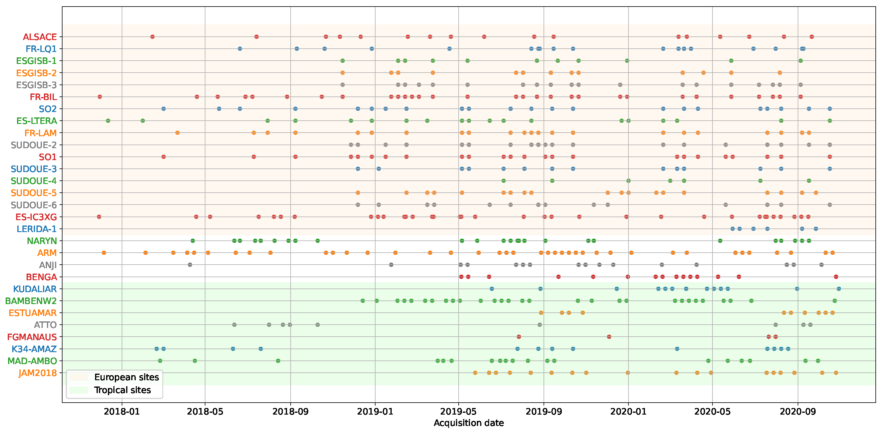
Figure 6 shows the distribution of acquisition dates for each site. The sites are sorted by decreasing latitude (from north to south). One can observe that for European sites, there is a drop in the number of pairs in the 2019–2020 winter season, while the 2018–2019 winter season is better sampled. In the 2018 fall season, one can also observe a drop in pairs density. This can be explained by the higher cloud cover in winter and fall in the northern hemisphere. Nevertheless, the dataset contains samples covering all seasons from late 2019 to September 2020. In tropical areas, the cloud cover is usually higher through the year, which results in large gaps in temporal coverage.
Sentinel-2 and Venµs are two sun-synchronous satellites, which means that their orbits always cross the equator at the same local time (10:30 a.m. for both Sentinel-2 and Venµs). Therefore, the difference in acquisition time for a given site should be very limited. This is highlighted in Figure 7, which shows the difference in acquisition time between Sentinel-2 and Venµs acquisitions for all pairs in the dataset, for each site. One can observe that this delta never exceeds 30 min, and for a good half of the sites, it is less than 10 min. For a given site, the range of deltas across pairs is very stable, and lower than 10 min for most sites.
2.5. Sampling Patches in Pairs
Each pair of VENµS and Sentinel-2 images identified in Section 2.4 underwent the same patch sampling procedure, which is further described in this section.
2.5.1. Reprojection and Common Bounding Box Cropping
Sentinel-2 image layouts follow the MGRS tile system, where each tile corresponds to a specific area using the local Universal Transverse Mercator (UTM) projection. VENµS data also follows the local UTM projection but with a grid specific to each site. A first step is therefore to determine the common bounding box between the Sentinel-2 and VENµS images.
2.5.2. Spatial Registration
It is well known that remote sensing sensors may suffer from absolute location error. According to ESA data quality reports, Sentinel-2 absolute location accuracy is 11 m for 95.5% of the products. Of course, this is prior to the new GRI processing that was set up in April 2021, but since the reprocessing is still ongoing, most products in the Theia archive will have this accuracy, which corresponds to two pixels from VENµS. On the VENµS side, partly because of the narrower field of view, accuracy is measured to be 3 m for 93% of the images [32]. Since the aim of the SEN2VENµS dataset is to serve for the training of super-resolution algorithms, correct alignments of images is of great importance. The following procedure has therefore been implemented to register the Sentinel-2 image onto the VENµS image of a given pair.
A global translation is estimated between the two images. This translation is estimated on the blue channel of both sensors, at 10 m resolution, which means that the VENµS image is first downsampled by a factor of two using a bicubic kernel.
To estimate the translation, the SIFT key-points detection and matching algorithms [33] have been used in a similar way as in [34]:
- Divide the downsampled VENµS image and the Sentinel-2 in non-overlapping corresponding patches of 366 × 366 pixels;
- For each patch, compute SIFT matches;
- Discard matches that are masked by the respective validity masks;
- Discard matches that are further that 15 m apart (obvious outliers);
- Compute the average shift in both directions from the collection of remaining matches.
The idea behind this process is that while individual SIFT matches are highly unreliable, estimating a two parameter transform from a collection of several thousands of points is reliable. In all cases, because of step 4), the applied shift magnitude will not be greater than 15 m.
Once the average shift is estimated, it is applied to the Sentinel-2 image with bicubic resampling to obtain registered Sentinel-2 images at both 10 m and 20 m.
2.5.3. Patchification and Invalid Patch Filtering
Once data have been registered, images are divided into corresponding triplets of patches. All 5 m bands from VENµS are divided into patches of 256 × 256 pixels. Consequently, the corresponding patches of Sentinel-2 10 m bands have a shape of 128 × 128 pixels, and the corresponding patches of Sentinel-2 20 m bands have a shape of 64 × 64 pixels.
If any pixel of any patch in the triplet (either VENµS 5 m, Sentinel-2 10 m or Sentinel-2 20 m) is invalid according to the corresponding validity mask, due to a detected cloud for instance, the triplet is entirely discarded, so that after this process all patches are composed of valid pixels only.
2.5.4. Radiometric Adjustments
Despite both Sentinel-2 and VENµS products being processed to level 2A, which includes atmospheric corrections, remaining differences in sensor spectral sensitivity responses (see Figure 1) as well as differences in acquisition angles (see Figure 4) and time (see Figure 7) will result in slight radiometric differences. Since the aim is to provide a dataset for the super-resolution of Sentinel-2 images, VENµS radiometries are adjusted to increase their coherence with Sentinel-2. Because those parameters can vary between sites and pairs, a separate adjustment is performed for each pair. A previous work [35] showed that linear regression was sufficient to compensate for discrepancies between surface reflectances from different sensors with similar spectral bands.
For each pair, a linear least-square radiometric fit is performed between all source and target bands, separately for the group of 10 m bands and the group of 20 m bands (see Table 1). This is described in Equation (1) for the 10 m bands, where W is a containing the linear regression weights, V is the source matrix containing n rows of VENµS surface reflectances from n randomly selected pixels, and S is the target matrix containing n rows of Sentinel2 surface reflectances in the corresponding bands. The equation holds separately for Sentinel-2 20 m bands.
VENµS patches are downscaled beforehand, so that the fit is performed at Sentinel-2 resolution. Prior to fitting, patches with a global RMSE greater than 0.2 reflectance count are discarded to avoid obvious outliers.
Note that the VENµS B11 band is processed twice and fitted separately to the wide near infrared B8 channel at 10 m and to the narrow near infrared B8A Sentinel-2 channel at 20 m (see Figure 1). This allows us to build consistent 5 m references for those two bands, as discussed in Section 3.2.
2.5.5. Random Selection and Outlier Removal
A random selection of at most 500 patches is performed for each pair, which in most cases samples all the valid patches, since a squared VENµS site should contain at most 484 patches. This allows us to limit the imbalance with respect to sites with a longer segment.
After this selection, a final outlier removal is carried out. This removal has been added afterward after finding some patches with spurious differences, such as unmasked cloud shadows or specular reflections. To eliminate those patches, any patch for which the RMSE between the Sentinel-2 10 m band and their corresponding VENµS bands downsampled at 10 m is greater than 0.02 has been discarded. This operation discards approximately 6.75% of the patches.
3. Dataset Content
In this section, the characteristics of the generated dataset are further described.
3.1. Quantitative Analysis
In total, the SEN2VENµS dataset contains 132,955 patches. Figure 8 presents the number of patches sampled from each site. One can observe that only five sites have more than 8 k patches, and that only the ARM site has more than 12 k patches. On the other hand, 16 sites have less than 4 k patches sampled. While this imbalance might be seen as problematic for the training of some algorithms, it must be stressed that this imbalance is different in nature than the classical class imbalance problem in classification tasks: what really matters is variability and equity of different kinds of landscape, which cannot be reduced to sites. For instance, several sites in southwest France will exhibit the same kind of landscape.
Figure 9 allows us to dig further into the sampling of each site. One can observe that if the maximum number of patches per pair reaches our 500 limit for most sites, the minimum is almost always very small because of pairs suffering from heavy cloud cover. Other sites, such as ARM in Oklahoma, USA, ESGIS-B3 in the west of France or LERIDA-1 in Spain show a median number of patches per pair close to the maximum, which denotes a fair sampling across pairs.
One important thing to know is whether VENµS 5 m patches are faithful to Sentinel-2 radiometry in each band, so as to avoid capturing radiometric biases in the course of a learning process involving the dataset. To answer this question, the mean average error and root mean square error have been computed in each band for a random selection of 200 patches involving at most 10 different pairs for each site, by first downsampling VENµS patches to the Sentinel-2 corresponding resolution (either 10 m or 20 m depending on the band). Downsampling is achieved by first convolving the 5 m image with a Gaussian spatial kernel whose standard deviation is tuned to the known values of the modulation transfer function at the Nyquist rate for Sentinel-2 and then decimating to the target resolution. Those metrics are presented in Figure 10 and Figure 11. The first thing to note from those two figures is that for all bands and all sites, mean average error is lower than the expected absolute surface reflectance error specification of the MAJA algorithm, which is set to 0.01 for all bands. It is therefore safe to say that the dataset has a good spectral consistency between Sentinel-2 and VENµS, for all bands. One can also observe that the Sentinel-2 B8 band is often the band with the higher MAE and RMSE, which can be explained by its lesser match with the VENµS band. Nevertheless, being the only 10 m band in the near infrared, it seemed reasonable to keep it in the dataset. One can also observe a tendency of the MAE error to increase with the zenith viewing angle, which may be explained by higher BRDF and parallax effects. This trend is not confirmed for all sites, however, as site BENGA, located in India, has almost the highest viewing angles and better performances than its high angle siblings. On the other hand, one can observe that the root mean square error does not show a clear trend related to the viewing angle, and that the root mean square error is quite stable across sites for a given spectral band. It is worth noting that all bands have a RMSE below 0.03 for all sites.
3.2. Qualitative Analysis
Figure 12 shows one sample patch per site, drawn at random. One can observe the variety of landscapes covered by the dataset, including natural, semi-natural and urban areas, as well as forest and shorelines. One can also observe the spectral consistency between Sentinel-2 (odd columns) and Venµs (even columns) patches. Note the high consistency of the 5 m B8 (columns 4 and 12) and B8A (columns 8 and 16) bands with their Sentinel-2 10 m (columns 3 and 11) and 20 m (columns 7 and 15) corresponding bands, though being generated from the same B11 VENµS band. The wider bandwidth B8 has less distinctive features, whereas B8 accurately responds to vegetated areas, and this difference is also visible in the 5 m reference patches.
Despite a very high consistency between VENµS and Sentinel-2 patches, local discrepancies remain between the 5 m VENµS patch and its corresponding 10 m or 20 m Sentinel-2 patch. For instance, when comparing A9 with A10, one can see cars on the road on the VENµS patch that have no match in the Sentinel-2 patch. Other differences include changes in water surfaces (C1 vs. C2), and artifacts related to viewing angles (shadowed area in G1 appear larger than in G2). Nevertheless, it must be stressed that those discrepancies are expected when using two different sensors as it is impossible to filter out or model all the differences between sensors specifications and viewing conditions. This dataset can be used as a real world case for algorithms, which should be resilient to those discrepancies.
3.3. Format and Distribution
The dataset is composed of separate sub-datasets, one for each site. For each site, the sub-dataset folder contains a set of files for each date, following this naming convention as the pair id: {site_name}_{mgrs_tile}_{acquisition_date}. For each pair, five files are available, as shown in Table 3. Patches are encoded as ready-to-use tensors as serialized by the well known Pytorch library [36]. As such, they can be loaded by a simple call to the torch.load() function. Note that bands are separated into two groups (10 m and 20 m Sentinel2 bands), which leads to four separate tensor files (two groups of bands × source and target resolution). Tensor shape is [n,c,w,h] where n is the number of patches, is the number of bands, w is the patch width and h is the patch height. To save storage space, they are encoded as 16 bit signed integers and should be converted back to floating point surface reflectance by dividing each and every value by 10,000 upon reading.
Each file comes with a master index.csv CSV (comma separated values) file, with one row for each pair sampled in the given site, and columns as described in Table 4, separated with tabs.
Figure 13 shows the size in gigabytes for each site in the dataset. Altogether the dataset weighs 116 Gb. Each site is compressed into a separate archive.
The SEN2VENµS dataset is distributed on Zenodo (https://zenodo.org/record/6514159) (accessed on 12 May 2022). Files {id}_05m_b2b3b4b8.pt and {id}_05m_b5 b6b7b8a.pt are distributed under the the original licence of the Sentinel-2 Theia L2A products, which is the Etalab Open Licence Version 2.0 (https://theia.cnes.fr/atdistrib/documents/Licence-Theia-CNES-Sentinel-ETALAB-v2.0-en.pdf) (accessed on 12 May 2022).
Files {id}_05m_b2b3b4b8.pt and {id}_05m_b5b6b7b8a.pt are distributed under the original licence of the VENµS products, which is Creative Commons BY-NC 4.0 (https://creativecommons.org/licenses/by-nc/4.0/) (accessed on 12 May 2022). Section 2.2. Remaining files are distributed under the Creative Commons BY 4.0 (https://creativecommons.org/licenses/by/4.0/) (accessed on 12 May 2022) licence.
Note that even if the SEN2VENµS dataset is sorted by sites and by pairs, it is strongly encouraged to apply the full set of machine learning best practices when using it: random keeping separate pairs (or even sites) for testing purposes and randomization of patches across sites and pairs in the training and validation sets.
4. Conclusions
SEN2VENµS is the first Single Image Super-Resolution open dataset to be made publicly available for the remote sensing research community. It is tailored for the training, evaluation and benchmarking of super-resolution algorithms for Sentinel-2 data, including red edge bands and narrow near infrared bands, and it targets the 5 m resolution for all bands, thanks to simultaneous VENµS 5 m acquisitions. SEN2VENµS covers a wide variety of seasons and landscapes across 2 years and 29 different sitesand exhibits a very strong radiometric consistency between the Sentinel-2 patches and their corresponding VENµS patches, with a top of canopy surface reflectance RMSE of at most 0.03 across all bands and sites. SEN2VENµS aims at becoming a reference dataset in the Single Image Super-Resolution for the remote sensing scientific community, and its strong radiometric consistency may be able to drive researchers toward better radiometric faithfulness of those methods.
As any dataset composed of real world data, the SEN2VENµS has some limitations and discrepancies that have been identified and analyzed in this paper. First, most sites are acquired from high viewing angles at 5 m (greater than 20°), whereas Sentinel-2 is acquired under at most 12°. This might cause differences in radiometry because of BRDF effects, and local misregistration because of parallax effects. A second limitation is the imbalance of number of dates and number of patches across sites. Though this cannot directly be related to an imbalance in landscape variability, extra care must be taken during training to avoid specialization on the most represented sites. Third, as any real world dataset, and despite all precautions taken during its preparation, additional discrepancies may occur for some individual patches, including rapid change of landscape between the low and high resolution acquisitions and spurious image quality artifacts. However, any super-resolution method aiming at operational use must be able to cope with such discrepancies.
Author Contributions
Conceptualization, J.M., O.H. and J.I.; methodology, J.M., O.H. and J.I.; software, J.M. and J.V.-S.; validation, J.M. and J.V.-S.; data curation, J.M. and J.V.-S.; writing—original draft preparation, J.M.; writing—review and editing, J.M., J.V.-S., O.H. and J.I. All authors have read and agreed to the published version of the manuscript.
Funding
This research was funded by CNES, Toulouse, in the frame of the Sentinel-HR phase-0 study.
Institutional Review Board Statement
Not applicable.
Informed Consent Statement
Not applicable.
Data Availability Statement
Dataset available at https://zenodo.org/record/6514159 (accessed on 12 May 2022).
Conflicts of Interest
The authors declare no conflict of interest.
References
- Lanaras, C.; Bioucas-Dias, J.; Baltsavias, E.; Schindler, K. Super-resolution of multispectral multiresolution images from a single sensor. In Proceedings of the IEEE Conference on Computer Vision and Pattern Recognition Workshops, Honolulu, HI, USA, 21–26 July 2017; pp. 20–28. [Google Scholar]
- Paris, C.; Bioucas-Dias, J.; Bruzzone, L. A hierarchical approach to superresolution of multispectral images with different spatial resolutions. In Proceedings of the 2017 IEEE International Geoscience and Remote Sensing Symposium (IGARSS), Fort Worth, TX, USA, 23–28 July 2017; pp. 2589–2592. [Google Scholar]
- Lin, C.H.; Bioucas-Dias, J.M. An explicit and scene-adapted definition of convex self-similarity prior with application to unsupervised Sentinel-2 super-resolution. IEEE Trans. Geosci. Remote Sens. 2019, 58, 3352–3365. [Google Scholar] [CrossRef]
- Gargiulo, M.; Mazza, A.; Gaetano, R.; Ruello, G.; Scarpa, G. Fast super-resolution of 20 m Sentinel-2 bands using convolutional neural networks. Remote Sens. 2019, 11, 2635. [Google Scholar] [CrossRef]
- Lanaras, C.; Bioucas-Dias, J.; Galliani, S.; Baltsavias, E.; Schindler, K. Super-resolution of Sentinel-2 images: Learning a globally applicable deep neural network. ISPRS J. Photogramm. Remote Sens. 2018, 146, 305–319. [Google Scholar] [CrossRef]
- Palsson, F.; Sveinsson, J.R.; Ulfarsson, M.O. Sentinel-2 Image Fusion Using a Deep Residual Network. Remote Sens. 2018, 10, 1290. [Google Scholar] [CrossRef]
- Nguyen, H.V.; Ulfarsson, M.O.; Sveinsson, J.R.; Dalla Mura, M. Sentinel-2 sharpening using a single unsupervised convolutional neural network with MTF-based degradation model. IEEE J. Sel. Top. Appl. Earth Obs. Remote Sens. 2021, 14, 6882–6896. [Google Scholar] [CrossRef]
- Ciotola, M.; Ragosta, M.; Poggi, G.; Scarpa, G. A full-resolution training framework for Sentinel-2 image fusion. In Proceedings of the 2021 IEEE International Geoscience and Remote Sensing Symposium IGARSS, Brussels, Belgium, 11–16 July 2021; pp. 1260–1263. [Google Scholar]
- Chan, T.; Wong, C.K. Total variation blind deconvolution. IEEE Trans. Image Process. 1998, 7, 370–375. [Google Scholar] [CrossRef]
- Krishnan, D.; Tay, T.; Fergus, R. Blind deconvolution using a normalized sparsity measure. In Proceedings of the CVPR 2011, Colorado Springs, CO, USA, 20–25 June 2011; pp. 233–240. [Google Scholar] [CrossRef]
- Anwar, S.; Khan, S.; Barnes, N. A deep journey into super-resolution: A survey. ACM Comput. Surv. (CSUR) 2020, 53, 1–34. [Google Scholar] [CrossRef]
- Liu, H.; Qian, Y.; Zhong, X.; Chen, L.; Yang, G. Research on super-resolution reconstruction of remote sensing images: A comprehensive review. Opt. Eng. 2021, 60, 100901. [Google Scholar] [CrossRef]
- Agustsson, E.; Timofte, R. Ntire 2017 challenge on single image super-resolution: Dataset and study. In Proceedings of the IEEE Conference on Computer Vision and Pattern Recognition Workshops, Honolulu, HI, USA, 21–26 July 2017; pp. 126–135. [Google Scholar]
- Shoeiby, M.; Robles-Kelly, A.; Wei, R.; Timofte, R. Pirm2018 challenge on spectral image super-resolution: Dataset and study. In Proceedings of the European Conference on Computer Vision (ECCV) Workshops, Munich, Germany, 8–14 September 2018. [Google Scholar]
- Wang, Y.; Wang, L.; Yang, J.; An, W.; Guo, Y. Flickr1024: A large-scale dataset for stereo image super-resolution. In Proceedings of the IEEE/CVF International Conference on Computer Vision Workshops, Long Beach, CA, USA, 16–17 June 2019. [Google Scholar]
- Rohith, G.; Kumar, L.S. Paradigm shifts in super-resolution techniques for remote sensing applications. Vis. Comput. 2021, 37, 1965–2008. [Google Scholar] [CrossRef]
- Pouliot, D.; Latifovic, R.; Pasher, J.; Duffe, J. Landsat super-resolution enhancement using convolution neural networks and Sentinel-2 for training. Remote Sens. 2018, 10, 394. [Google Scholar] [CrossRef]
- Galar, M.; Sesma, R.; Ayala, C.; Aranda, C. Super-Resolution for Sentinel-2 Images. Int. Arch. Photogramm. Remote Sens. Spat. Inf. Sci. 2019, XLII-2/W16, 95–102. [Google Scholar] [CrossRef]
- Salgueiro Romero, L.; Marcello, J.; Vilaplana, V. Super-resolution of sentinel-2 imagery using generative adversarial networks. Remote Sens. 2020, 12, 2424. [Google Scholar] [CrossRef]
- Pineda, F.; Ayma, V.; Beltran, C. A generative adversarial network approach for super-resolution of sentinel-2 satellite images. Int. Arch. Photogramm. Remote Sens. Spat. Inf. Sci. 2020, 43, 9–14. [Google Scholar] [CrossRef]
- Tao, Y.; Xiong, S.; Song, R.; Muller, J.P. Towards Streamlined Single-Image Super-Resolution: Demonstration with 10 m Sentinel-2 Colour and 10–60 m Multi-Spectral VNIR and SWIR Bands. Remote Sens. 2021, 13, 2614. [Google Scholar] [CrossRef]
- Galar, M.; Sesma, R.; Ayala, C.; Albizua, L.; Aranda, C. Super-resolution of sentinel-2 images using convolutional neural networks and real ground truth data. Remote Sens. 2020, 12, 2941. [Google Scholar] [CrossRef]
- Märtens, M.; Izzo, D.; Krzic, A.; Cox, D. Super-resolution of PROBA-V images using convolutional neural networks. Astrodynamics 2019, 3, 387–402. [Google Scholar] [CrossRef]
- Drusch, M.; Del Bello, U.; Carlier, S.; Colin, O.; Fernandez, V.; Gascon, F.; Hoersch, B.; Isola, C.; Laberinti, P.; Martimort, P.; et al. Sentinel-2: ESA’s optical high-resolution mission for GMES operational services. Remote Sens. Environ. 2012, 120, 25–36. [Google Scholar] [CrossRef]
- Phiri, D.; Simwanda, M.; Salekin, S.; Nyirenda, V.R.; Murayama, Y.; Ranagalage, M. Sentinel-2 data for land cover/use mapping: A review. Remote Sens. 2020, 12, 2291. [Google Scholar] [CrossRef]
- Segarra, J.; Buchaillot, M.L.; Araus, J.L.; Kefauver, S.C. Remote sensing for precision agriculture: Sentinel-2 improved features and applications. Agronomy 2020, 10, 641. [Google Scholar] [CrossRef]
- Misra, G.; Cawkwell, F.; Wingler, A. Status of phenological research using Sentinel-2 data: A review. Remote Sens. 2020, 12, 2760. [Google Scholar] [CrossRef]
- Ferrier, P.; Crebassol, P.; Dedieu, G.; Hagolle, O.; Meygret, A.; Tinto, F.; Yaniv, Y.; Herscovitz, J. VENμS (Vegetation and environment monitoring on a new micro satellite). In Proceedings of the 2010 IEEE International Geoscience and Remote Sensing Symposium, Honolulu, HI, USA, 25–30 July 2010; pp. 3736–3739. [Google Scholar]
- Dedieu, G.; Hagolle, O.; Karnieli, A.; Ferrier, P.; Crébassol, P.; Gamet, P.; Desjardins, C.; Yakov, M.; Cohen, M.; Hayun, E. VENµS: Performances and First Results after 11 Months in Orbit. In Proceedings of the IGARSS 2018—2018 IEEE International Geoscience and Remote Sensing Symposium, Valencia, Spain, 22–27 July 2018; pp. 7756–7759. [Google Scholar] [CrossRef]
- Lonjou, V.; Desjardins, C.; Hagolle, O.; Petrucci, B.; Tremas, T.; Dejus, M.; Makarau, A.; Auer, S. Maccs-atcor joint algorithm (maja). In Proceedings of the Remote Sensing of Clouds and the Atmosphere XXI; International Society for Optics and Photonics: Bellingham, WA, USA, 2016; Volume 10001, p. 1000107. [Google Scholar]
- Buchhorn, M.; Smets, B.; Bertels, L.; Roo, B.D.; Lesiv, M.; Tsendbazar, N.E.; Herold, M.; Fritz, S. Copernicus Global Land Service: Land Cover 100m: Collection 3: Epoch 2019: Globe. 2020. Available online: https://0-doi-org.brum.beds.ac.uk/10.5281/zenodo.3939050 (accessed on 12 May 2022).
- Dick, A.; Raynaud, J.L.; Rolland, A.; Pelou, S.; Coustance, S.; Dedieu, G.; Hagolle, O.; Burochin, J.P.; Binet, R.; Moreau, A. VENμS: Mission Characteristics, Final Evaluation of the First Phase and Data Production. Remote Sens. 2022, 14, 3281. [Google Scholar] [CrossRef]
- Lowe, G. Sift-the scale invariant feature transform. Int. J. 2004, 2, 2. [Google Scholar]
- Michel, J.; Sarrazin, E.; Youssefi, D.; Cournet, M.; Buffe, F.; Delvit, J.; Emilien, A.; Bosman, J.; Melet, O.; L’Helguen, C. A new satellite imagery stereo pipeline designed for scalability, robustness and performance. ISPRS Ann. Photogramm. Remote Sens. Spat. Inf. Sci. 2020, 2, 171–178. [Google Scholar] [CrossRef]
- Michel, J.; Inglada, J. Learning Harmonised Pleiades and SENTINEL-2 Surface Reflectances. Int. Arch. Photogramm. Remote Sens. Spat. Inf. Sci. 2021, 43, 265–272. [Google Scholar] [CrossRef]
- Paszke, A.; Gross, S.; Massa, F.; Lerer, A.; Bradbury, J.; Chanan, G.; Killeen, T.; Lin, Z.; Gimelshein, N.; Antiga, L.; et al. PyTorch: An Imperative Style, High-Performance Deep Learning Library. In Advances in Neural Information Processing Systems 32; Wallach, H., Larochelle, H., Beygelzimer, A., d’Alché-Buc, F., Fox, E., Garnett, R., Eds.; Curran Associates, Inc.: Red Hook, NY, USA, 2019; pp. 8024–8035. [Google Scholar]
- Michel, J.; Hagolle, O.; Puissant, A.; Herrault, P.A.; Corpetti, T.; Nabucet, J.; Faure, J.F.; Maurel, P.; Lelong, C.; Berthier, E.; et al. Sentinel-HR Phase 0 Report; Research Report; CNES-Centre National d’études Spatiales; CESBIO: Singapore, 2022. [Google Scholar]
- Ahn, N.; Kang, B.; Sohn, K.A. Fast, accurate, and lightweight super-resolution with cascading residual network. In Proceedings of the European Conference on Computer Vision (ECCV), Munich, Germany, 8–14 September 2018; pp. 252–268. [Google Scholar]
Figure 1.
Spectral sensitivity response of corresponding spectral bands between Sentinel-2 (top) and VENµS (bottom).
Figure 1.
Spectral sensitivity response of corresponding spectral bands between Sentinel-2 (top) and VENµS (bottom).

Figure 2.
Map of Sentinel-2 coverage on Theia (orange), available VENµS sites (green) and 29 selected sites (red) for the dataset.
Figure 2.
Map of Sentinel-2 coverage on Theia (orange), available VENµS sites (green) and 29 selected sites (red) for the dataset.

Figure 3.
Proportions of Copernicus 2019 Land-Cover [31] classes for each site. Sites are sorted by decreasing latitude (from north to south).
Figure 3.
Proportions of Copernicus 2019 Land-Cover [31] classes for each site. Sites are sorted by decreasing latitude (from north to south).

Figure 4.
Zenith viewing angles for the 29 selected VENµS sites.

Figure 5.
Distribution of the 579 selected pairs across selected VENµS sites, sorted by increasing zenith viewing angle.
Figure 5.
Distribution of the 579 selected pairs across selected VENµS sites, sorted by increasing zenith viewing angle.

Figure 6.
Distribution of acquisition dates of selected pairs for each site. Colors are used to increase readability. Sites are sorted by decreasing latitude (from north to south). European and equatorial sites are distinguished with background colors (light orange for European, light green for equatorial) to assess seasonal coverage.

Figure 7.
Distribution of time deltas in minutes between Venµs and Sentinel-2 local time (if negative, Venµs acquisition is later than Sentinel-2 acquisition). Colors are used to increase readibility. Sites are sorted by decreasing latitude (from north to south).
Figure 7.
Distribution of time deltas in minutes between Venµs and Sentinel-2 local time (if negative, Venµs acquisition is later than Sentinel-2 acquisition). Colors are used to increase readibility. Sites are sorted by decreasing latitude (from north to south).

Figure 8.
Total number of patches sampled from each site.

Figure 9.
Statistics of number of patches per pair for each site.

Figure 10.
Mean average error per band and per site computed on a random selection of 200 patches from at most 20 pairs at Sentinel-2 resolution.
Figure 10.
Mean average error per band and per site computed on a random selection of 200 patches from at most 20 pairs at Sentinel-2 resolution.

Figure 11.
Root mean square error per band and per site computed on a random selection of 200 patches from at most 20 pairs at Sentinel-2 resolution.
Figure 11.
Root mean square error per band and per site computed on a random selection of 200 patches from at most 20 pairs at Sentinel-2 resolution.

Figure 12.
Examples of patches from left to right: columns 1–8 and 9–16 show rendering of two different patches; columns 1 and 9: B4, B3, B7 (RGB natural) at 10 m; columns 2 and 10: B4, B3, B7 (RGB natural) at 5 m; columns 3 and 11: color-mapped B8 at 10 m (wide near infrared); columns 4 and 12: color-mapped B8 at 5m (wide near infrared); columns 5 and 13: B7, B6, B5 color composition (red edge 3 to 1) at 20 m; columns 6 and 14: B7, B6, B5 color composition (red edge 3 to 1) at 5 m; columns 7 and 15: color-mapped B8A at 20 m (narrow near infrared), columns 8 and 16: color-mapped B8A at 5 m (narrow near infrared). A total of 29 patches are displayed, one random patch for each site. Only 64 × 64 pixels crops of the patches are displayed to improve readability. High resolution and low resolution patches radiometries where scaled to 8 bits with the same scaling factors.

Figure 13.
Uncompressed files sizes for each site in gigabytes. The full dataset weighs 116 Gb.


Table 1.
Corresponding Sentinel-2 and VENµS bands used in the SEN2VENµS dataset. Note that B11 is used as a high resolution band for both B8 and B8A Sentinel-2 bands.
Table 1.
Corresponding Sentinel-2 and VENµS bands used in the SEN2VENµS dataset. Note that B11 is used as a high resolution band for both B8 and B8A Sentinel-2 bands.
| Sentinel-2 | 10 m bands | 20 m bands |
| B2 B3 B4 B8 | B5 B6 B7 B8A | |
| VENµS | 5 m bands | 5 m bands |
| B3 B4 B7 B11 | B8 B9 B10 B11 |
Table 2.
Country and province of each of the selected VENµS sites, sorted by decreasing latitude (from north to south).
Table 2.
Country and province of each of the selected VENµS sites, sorted by decreasing latitude (from north to south).
| Site Name | Country | Province | Longitude | Latitude |
|---|---|---|---|---|
| ALSACE | France | Alsace | 7.46897 | 48.379 |
| FR-LQ1 | France | Auvergne | 2.72879 | 45.6397 |
| ESGISB-1 | France | Aquitaine | −0.692399 | 45.1198 |
| ESGISB-2 | France | Aquitaine | −0.767621 | 44.869 |
| ESGISB-3 | France | Aquitaine | −0.865341 | 44.5389 |
| FR-BIL | France | Aquitaine | −0.959032 | 44.49 |
| SO2 | France | Midi-Pyrenees | 1.26464 | 43.6105 |
| ES-LTERA | France | Midi-Pyrenees | 1.23902 | 43.5 |
| FR-LAM | France | Midi-Pyrenees | 1.17814 | 43.44 |
| SUDOUE-2 | France | Midi-Pyrenees | 1.09625 | 43.0986 |
| SO1 | France | Midi-Pyrenees | 1.02816 | 42.97 |
| SUDOUE-3 | France | Midi-Pyrenees | 1.01046 | 42.836 |
| SUDOUE-4 | Spain | Catalonia | 0.924987 | 42.5734 |
| SUDOUE-5 | Spain | Catalonia | 0.857221 | 42.3638 |
| SUDOUE-6 | Spain | Catalonia | 0.742541 | 41.9899 |
| ES-IC3XG | Spain | Galicia | −8.0173 | 41.9893 |
| LERIDA-1 | Spain | Catalonia | 0.636121 | 41.6624 |
| NARYN | Kyrgyzstan | Naryn | 76.5615 | 41.6096 |
| ARM | United States of America | Oklahoma | −97.4884 | 36.6097 |
| ANJI | China | Zhejiang Sheng | 119.839 | 30.58 |
| BENGA | India | West Bengal | 87.6132 | 23.609 |
| KUDALIAR | India | Telangana | 78.6974 | 17.9402 |
| BAMBENW2 | Senegal | Diourbel | −16.3837 | 14.6176 |
| ESTUAMAR | French Guyana | Guyane | −54.038 | 5.58975 |
| ATTO | Brazil | Amazonas | −59.0103 | −2.15005 |
| FGMANAUS | Brazil | Amazonas | −59.7905 | −2.43994 |
| K34-AMAZ | Brazil | Amazonas | −60.2103 | −2.6098 |
| MAD-AMBO | Madagascar | Vakinankaratra | 47.1392 | −19.6701 |
| JAM2018 | Brazil | Sao Paulo | −47.5153 | −22.7496 |
Table 3.
Naming convention for files associated to each pair. {id} is {site_name}_{mgrs_tile}_{acquisition_date}.
Table 3.
Naming convention for files associated to each pair. {id} is {site_name}_{mgrs_tile}_{acquisition_date}.
| File | Content |
|---|---|
| {id}_05m_b2b3b4b8.pt | 5 m patches ( pix.) for S2 B2, B3, B4 and B8 |
| {id}_10m_b2b3b4b8.pt | 10 m patches ( pix.) for S2 B2, B3, B4 and B8 |
| {id}_05m_b5b6b7b8a.pt | 5 m patches ( pix.) for S2 B5, B6, B7 and B8A |
| {id}_20m_b5b6b7b8a.pt | 20 m patches ( pix.) for S2 B5, B6, B7 and B8A |
| {id}_patches.gpkg | GIS file with footprint of each patch |
Table 4.
Columns of the index.csv file indexing pairs for each site. For file naming conventions, refer to Table 3.
Table 4.
Columns of the index.csv file indexing pairs for each site. For file naming conventions, refer to Table 3.
| Column | Description |
|---|---|
| venus_product_id | ID of the sampled VENµS L2A product |
| sentinel2_product_id | ID of the sampled Sentinel-2 L2A product |
| tensor_05m_b2b3b4b8 | Name of the 5 m tensor file for S2 B2, B3, B4 and B8 |
| tensor_10m_b2b3b4b8 | Name of the 10 m tensor file for S2 B2, B3, B4 and B8 |
| tensor_05m_b5b6b7b8a | Name of the 5 m tensor file for S2 B5, B6, B7 and B8A |
| tensor_20m_b5b6b7b8a | Name of the 20 m tensor file for S2 B5, B6, B7 and B8A |
| s2_tile | Sentinel-2 MGRS tile |
| vns_site | Name of VENµS site |
| date | Acquisition date as YYYY-MM-DD |
| venus_zenith_angle | VENµS zenith viewing angle in degrees |
| patches_gpkg | Name of the GIS file with footprint for each patch |
| nb_patches | Number of patches for this pair |
Publisher’s Note: MDPI stays neutral with regard to jurisdictional claims in published maps and institutional affiliations. |
© 2022 by the authors. Licensee MDPI, Basel, Switzerland. This article is an open access article distributed under the terms and conditions of the Creative Commons Attribution (CC BY) license (https://creativecommons.org/licenses/by/4.0/).
Share and Cite
MDPI and ACS Style
Michel, J.; Vinasco-Salinas, J.; Inglada, J.; Hagolle, O. SEN2VENµS, a Dataset for the Training of Sentinel-2 Super-Resolution Algorithms. Data 2022, 7, 96. https://0-doi-org.brum.beds.ac.uk/10.3390/data7070096
AMA Style
Michel J, Vinasco-Salinas J, Inglada J, Hagolle O. SEN2VENµS, a Dataset for the Training of Sentinel-2 Super-Resolution Algorithms. Data. 2022; 7(7):96. https://0-doi-org.brum.beds.ac.uk/10.3390/data7070096
Chicago/Turabian StyleMichel, Julien, Juan Vinasco-Salinas, Jordi Inglada, and Olivier Hagolle. 2022. "SEN2VENµS, a Dataset for the Training of Sentinel-2 Super-Resolution Algorithms" Data 7, no. 7: 96. https://0-doi-org.brum.beds.ac.uk/10.3390/data7070096