
Chroma Enhancement in CIELAB Color Space Using a Lookup Table


1
Department of Culture and Creative Arts, Yamaguchi Prefectural University, Yamaguchi 753-8502, Japan
2
Graduate School of Sciences and Technology for Innovation, Yamaguchi University, Yamaguchi 753-8512, Japan
*
Author to whom correspondence should be addressed.
Designs 2021, 5(2), 32; https://0-doi-org.brum.beds.ac.uk/10.3390/designs5020032
Submission received: 16 March 2021
/
Revised: 19 April 2021
/
Accepted: 10 May 2021
/
Published: 14 May 2021
(This article belongs to the Section Electrical Engineering Design)
Abstract
:In this study, we present a method of chroma enhancement in the CIELAB color space and compare it with that in the RGB color space. Color image enhancement using the CIELAB color space has the disadvantage that the color gamut problem occurs because the conversion to the RGB color space is necessary to display the image. However, since the CIELAB color space is based on human visual perception, the quality of the resulting images is expected to be higher than that of the RGB color space. In the method using the CIELAB color space, we introduce a lookup table to reduce the calculation costs. Experiments comparing image enhancement results obtained from two color spaces are performed using several digital images.
1. Introduction
Color digital images have been used in various situations in daily life due to the development of digital devices and Internet technologies. Therefore, it is necessary to improve the quality of these color digital images depending on their application [1,2].
The choice of color space when performing color image enhancement is an important factor that influences the quality of the resulting images [3]. The RGB color space is a typical color space for digital image processing. An arbitrary color in the RGB color space is represented by the ratio of the three primary colors of R (red), G (green), and B (blue). Meanwhile, the three attributes of color (i.e., hue, chroma, and lightness) are more useful when specifying a certain color based on human sensitivities than the RGB components [4]. These three attributes of color can also be geometrically defined in the RGB color space. Naik et al. clarified the conditions for preserving the hue in the RGB color space and demonstrated the method of image enhancement with its conditions [5]. Furthermore, several image enhancement methods have been proposed with reference to Naik’s method [6,7,8,9,10,11,12,13]. These methods make it possible to suppress hue distortion when image enhancement is applied in the RGB color space. Color image enhancement in the RGB color space has the advantage of not causing the color gamut problem, because the conversion to other color spaces is unnecessary. Furthermore, the relationship between hue, chroma, and lightness is easy to formulate, and the algorithm for color image enhancement can be expressed simply. However, since these attributes defined in the RGB color space are not based on human visual perception as in uniform color spaces, the quality of the resulting images may not be sufficient.
When focusing on human visual perception, the color spaces that can directly represent colors by using hue, chroma, and lightness, such as the HSI [14,15,16,17,18] and CIELAB [19,20,21,22,23,24,25] color spaces, are more useful than the RGB color space. Previously, we proposed an image enhancement method in the CIELAB color space, which is one of the uniform color spaces. In our previous method [22], a color gamut adjustment is applied to address the problem that may occur when inversely converting processed color components in the CIELAB color space to the RGB color space. However, in this method, there is a problem in that the calculation cost is high because it is necessary to solve the third-order polynomial for the pixels outside the color gamut. In this study, we introduce a lookup table that stores the maximum chroma values at sample points of hue and lightness. Finally, we compare the results obtained from the methods using the RGB and CIELAB color spaces.
The remainder of this paper is organized as follows: Section 2 and Section 3 explain the chroma enhancement methods in the RGB and CIELAB color spaces, respectively. In Section 4, a lookup table introduced in a method using CIELAB color space is described. Section 5 provides the experimental results of applying the proposed chroma enhancement methods to several digital images. Section 6 presents the conclusions of our study.
2. Chroma Enhancement in RGB Color Space
The RGB color space is usually used to represent color digital images acquired by various digital devices. In this section, we describe a method to enhance the chroma while preserving the hue and lightness in the RGB color space.
2.1. Equal Hue and Equal Lightness in RGB Color Space
In this study, sRGB is assumed as the RGB color space. Let be the input digital image at the pixel . have the three RGB components . Here, each RGB component is assumed to be normalized to the interval . For simplicity of notation, we omit after this.
Let J be the RGB color components after applying color image enhancement to I. When J have the same hue as I, they are obtained as follows [5]:
where . Equation (1) is the plane equation passing through and I with the parameters and . The lightness of I is given by the inner product of I and :
In our previous method [11], we employed . In this study, to correspond to the lightness defined in the CIELAB color space, let V be (0.2126, 0.7152, 0.0722), where .
Here, the lightness is kept at l before and after color image enhancement. That is,
By calculating the inner products of both sides of Equation (1) and V, and substituting Equations (2) and (3) for the calculation result, we get
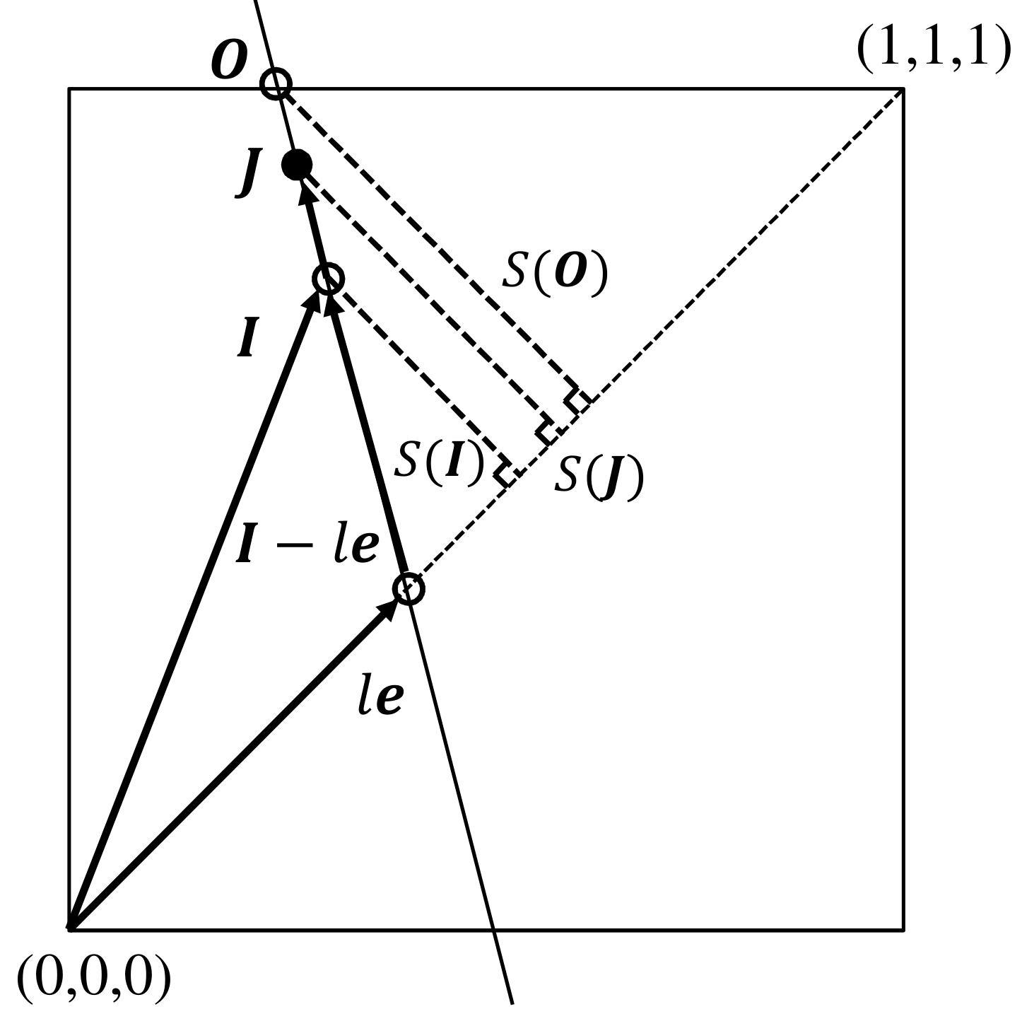
The chroma enhancement is executed by selecting the appropriate RGB color components on the straight line J (Figure 1).
2.2. Chroma in RGB Color Space
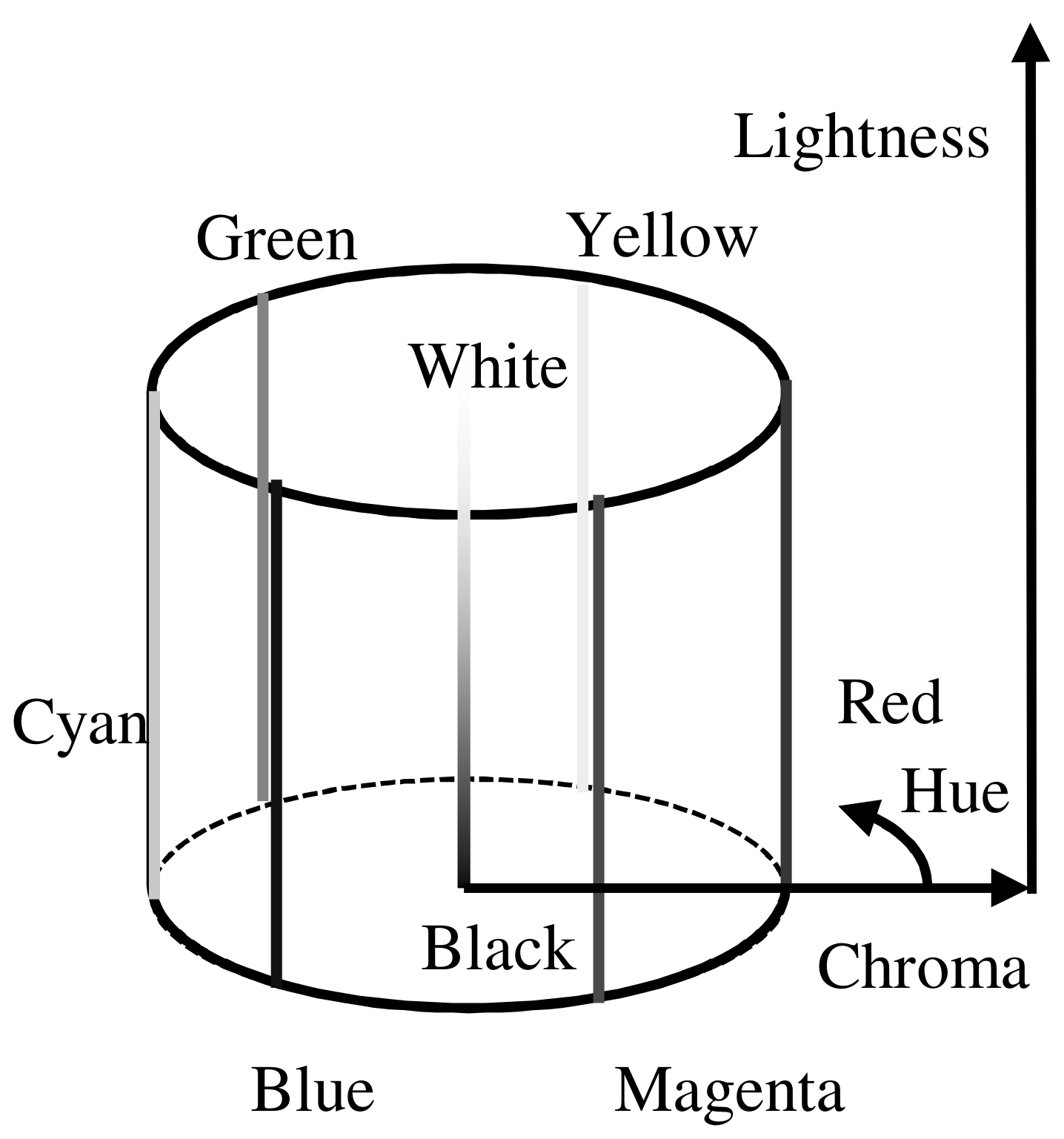
In the HSI color space with a cylindrical coordinate system (Figure 2), the hue, H, and the chroma, S, are obtained as follows [26]:
From Equations (5) and (6), = . This indicates that the hue is preserved after the chroma enhancement.
In addition, S() can be rewritten as
where indicates the Euclidean distance. Equation (8) represents the distance between I and the achromatic axis, e, as shown in Figure 1. That is, the chroma of a color in the RGB color space increases as the color moves away from the achromatic axis, e. Thus, from Equation (5), the chroma of J becomes larger than that of I as increases from 1.
Figure 2.
HSI color space with cylindrical coordinate system.

2.3. Chroma Enhancement Method
Let O be the intersection point between the straight line, J, and the boundary surface of the RGB color space. O has the maximum chroma among the colors that are of equal hue and equal lightness with the input color, I. The enhanced color is decided by using the distance, , as follows:
Here, is obtained as
where is the parameter that determines the degree of the chroma enhancement. J coincides with I when and coincides with O having the maximum chroma when owing to . Hence, by setting the parameter to a value larger than 1, we get a color with a chroma larger than that of the input color, I.
3. Chroma Enhancement in CIELAB Color Space
The definitions of hue, chroma, and, lightness in the RGB color space may not exactly match human visual perception because it is not a uniform color space. In this section, we present a method to enhance the chroma while preserving the hue and lightness in the CIELAB color space, which is one of the uniform color spaces.
Let be the input value of a nonlinear RGB component. E takes any one of r, g, and b, which indicate the red, green, and blue components, respectively. The nonlinear RGB component is converted to the linear RGB component as follows [27]:
The RGB color components, , are first converted to the CIEXYZ color components, , by the following linear transformation:
Next, are converted to the CIELAB color components, , by the following nonlinear transformation [28]:
where the function, f, is defined by
Here, is the lightness, and and represent the chromaticity indices of redness, greenness and yellowness, and blueness. and are the CIEXYZ values for the reference white of the illuminant CIE D65 and are 0.9505, 1.000, and 1.089, respectively. Note that , , and and . The chroma, , and the hue, h, in the CIELAB color space are obtained by and , respectively. Here, and . In this study, let in the case of because h becomes very sensitive to the change in or when is very small.
The chroma enhancement is conducted in the CIELAB color space while preserving the hue. The enhanced chroma, , is obtained by
where k is the parameter that determines the degree of the chroma enhancement. When applying the chroma enhancement by Equation (17), the hue, h, is preserved regardless of the value of k owing to . When the lightness is not changed before and after image enhancement, the CIELAB color components after the chroma enhancement are given by . The final RGB color components, , are obtained by converting to the RGB color space. However, it is unknown whether is within the color gamut of the RGB color space. Therefore, it is necessary to address the color gamut problem.
4. Color Gamut Adjustment after Chroma Enhancement Using Lookup Table
When image enhancement is conducted in the CIELAB color space, some pixels of the enhanced image may not be correctly converted into the RGB color space. In this section, as a solution to this problem, we propose a method of color gamut adjustment using a lookup table.
4.1. Relationship among Hue, Chroma, and Lightness
In our previous method [22], to handle the color gamut problem, Equations (14) and (15) are reformulated using variables related to hue, chroma, and lightness as follows:
where and is the sign function defined as follows:
and are the equations of straight lines with as a variable when H and , which are related to the hue and lightness, are fixed. Therefore, the color gamut problem is solved by finding the maximum value of at arbitrary hue and lightness.
4.2. Preparation of Lookup Table
We proposed a color gamut adjustment method that obtains the maximum chroma values while preserving the lightness and hue according to the range of Y. However, our previous method has a problem in that the calculation cost is high because it is necessary to solve the third-order polynomial for the pixels outside the color gamut.
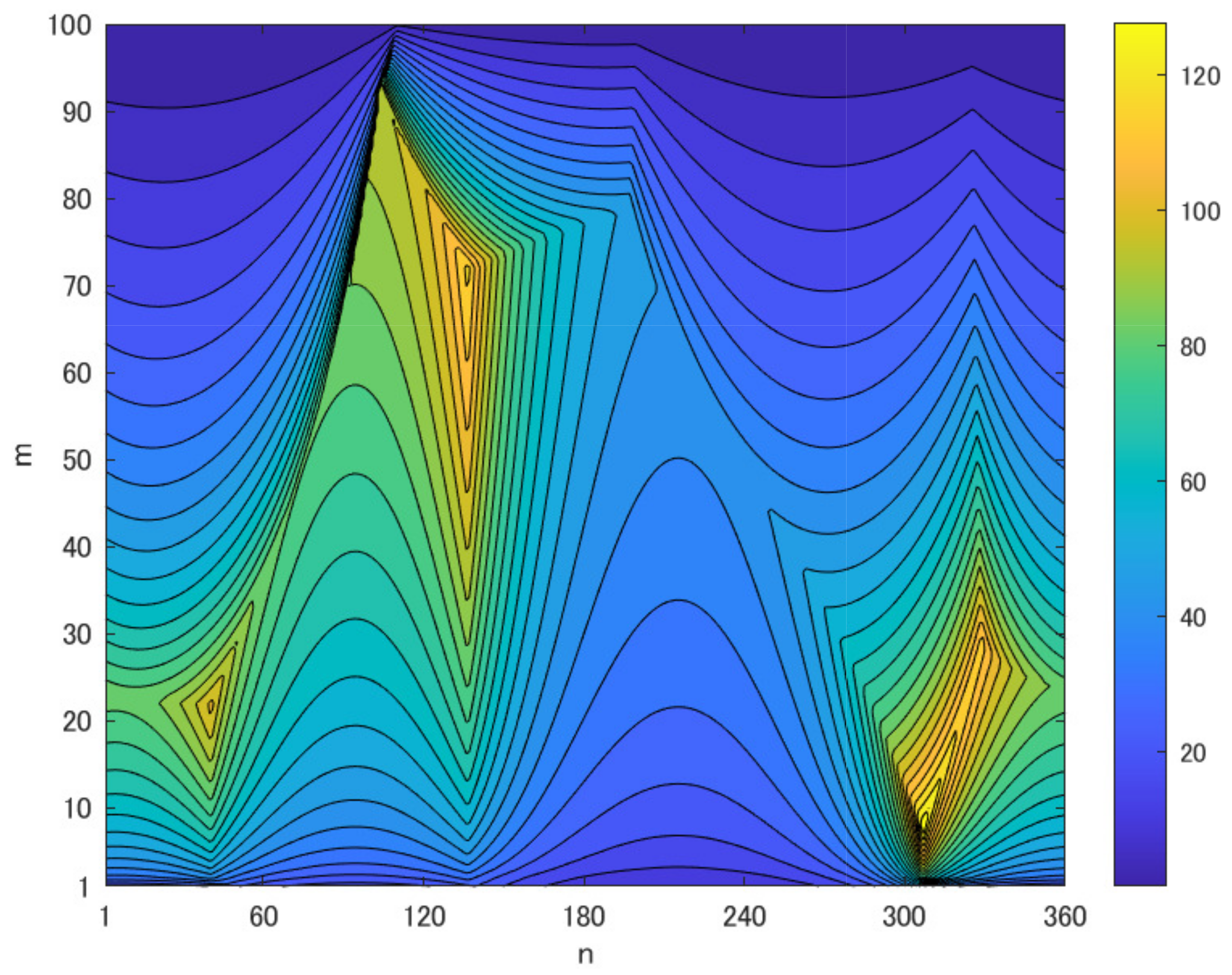
Therefore, we introduced a lookup table to reduce the calculation cost. The lookup table stores the maximum chroma values at the sampled Y and h. The procedure of making the lookup table is as follows: First, Y and h are sampled at 100 points from 0.005 to 0.995 with a step of 0.01 and at 360 points from 0.5 to 359.5 with a step of 1, respectively. Next, the maximum chroma values are calculated at these 36,000 points of using our previous method. Let be the element of the lookup table, where and . stores the maximum chroma value at the point, (, ). Figure 3 shows the lookup table obtained by the above procedure. This indicates the maximum chroma for a given hue and lightness.
4.3. Determination Method for Maximum Chroma Value Using Lookup Table
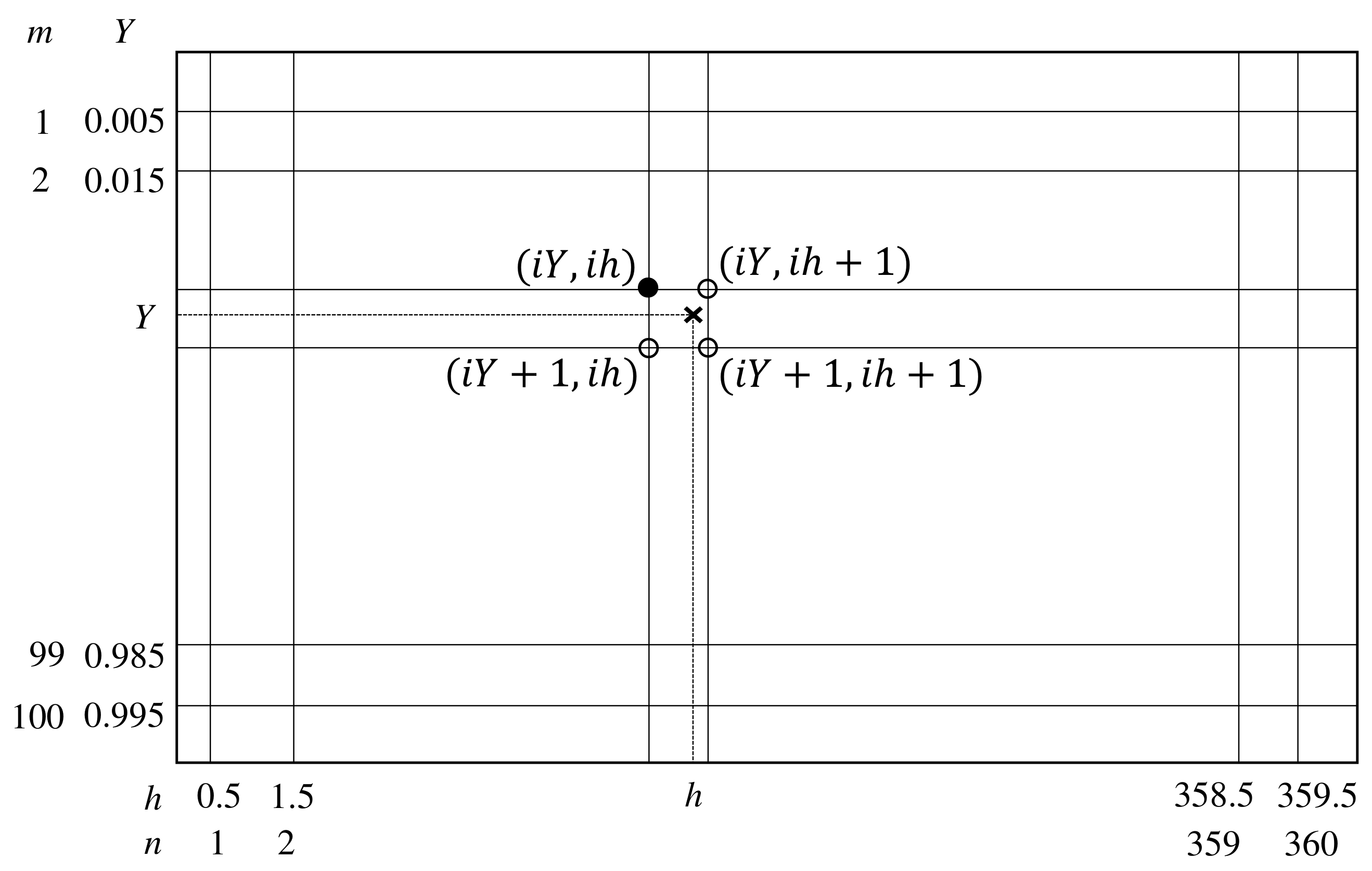
The approximate maximum chroma value of an arbitrary point, , can be obtained by the lookup table. Y and h are first converted to the integers as follows:
where is the function that rounds to the nearest integer.
The point is located inside the quadrangle with four vertices, namely, , , , and , as shown in Figure 4. Therefore, in the proposed method, the maximum chroma value of the point, , is assigned the minimum value among the four elements of the lookup table on the above points as follows:
where is the function that finds the minimum value in any given data. However, is set to 0 when and , corresponding to black and white. In addition, when and , the following formula is used
4.4. RGB Components after Color Gamut Adjustment
The approximate maximum chroma of the color gamut that is determined by h and Y is extracted from the lookup table by the procedure in Section 4.3. Substituting for Equations (18) and (19), we get
Here, is defined as follows:
are obtained by converting (, Y, ) to the RGB color space by using the inverse of the matrix used in Equation (12):
Finally, the nonlinear RGB component of the output image is obtained as
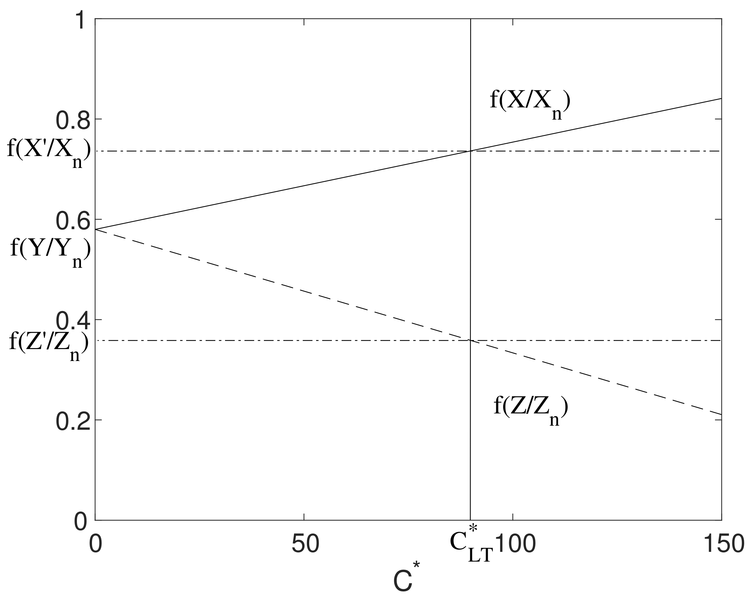
Figure 5.
and plotted as a function of at (, ). In this case, is 89.941.

5. Experiments
5.1. Chroma Enhancement
To illustrate the effectiveness of the proposed method, experiments are conducted using seven digital images: Pepper, Mandrill, Sailboat, Airplane, Balloon, Earth, and Lenna [29]. These are 24-bit color images of 256 × 256 pixels in size.
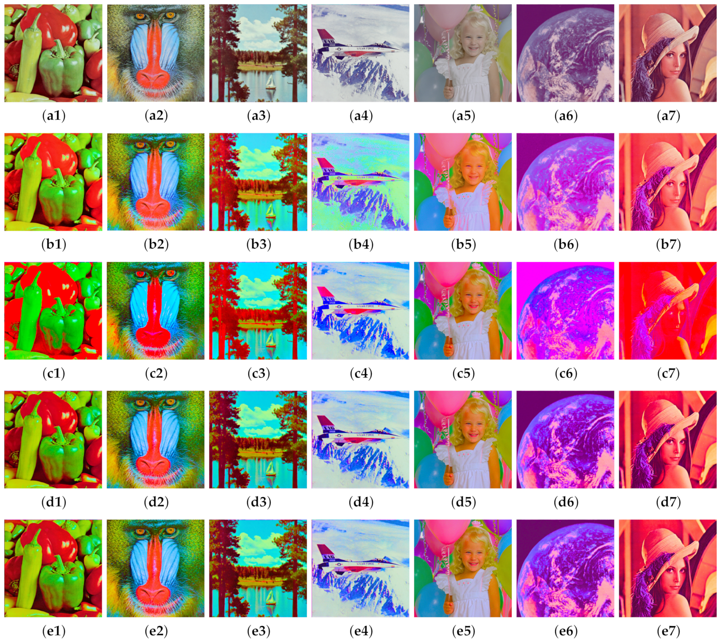
Figure A1 shows the experimental results of seven digital images. We can see that the large red bell peppers in Figure A1d1,e1 are deeper red than that in Figure A1b1. In addition, the blue part of the mandrill’s face in Figure A1d2,e2, the trunks and branches of the trees in Figure A1d3,e3, the clouds in Figure A1d4,e4, and the Earth in Figure A1d6,e6 are not over-enhanced compared to those in Figure A1b2–b4,b6.
To evaluate the quality of enhanced images from a perceptual point of view objectively, the difference related to hue between the enhanced and original images is calculated as follows [30]:
where and are the hues of the corresponding pixels in the enhanced and original images, respectively. Similarly, and refer to the chromas. is the absolute value. In addition, the differences, and , related to lightness and chroma are calculated to confirm the degree of image enhancement. Here, and refer to the lightnesses in the same meaning as above.
Table A1 shows the averages and standard deviations of , , and over all pixels in Figure A1. From the results of , we can see that and of the proposed method (e1–e7) are not so different from that of our previous method (d1–d7). In addition, the limitation of our previous method is trying to approximate Equation (16) by when applying color gamut adjustment. Therefore, when the lightness is very low, it becomes an approximate solution [22]. Since the present method using the lookup table selects the minimum chroma value among the four surrounding elements, the resulting color is highly likely to exist within the color gamut, and then it is thought that becomes smaller than that of our previous method. That is, the lookup table can achieve the image enhancement without significantly deteriorating the quality.
5.2. Combination of Lightness and Chroma Enhancement
The advantage of using the CIELAB color space compared to the RGB color space is that the chroma and lightness components are completely independent. The proposed lookup table can also be applied when both the lightness and chroma are enhanced. Here, the lightness is enhanced as follows:
where p is the parameter that determines the degree of lightness enhancement.
The proposed method is compared with the method of Ref. [5] using histogram equalization, the method of Ref. [7] using the parameters = (, , ) [31], and the RGB chroma enhancement in Section 2, in which histogram equalization is applied to the lightness.
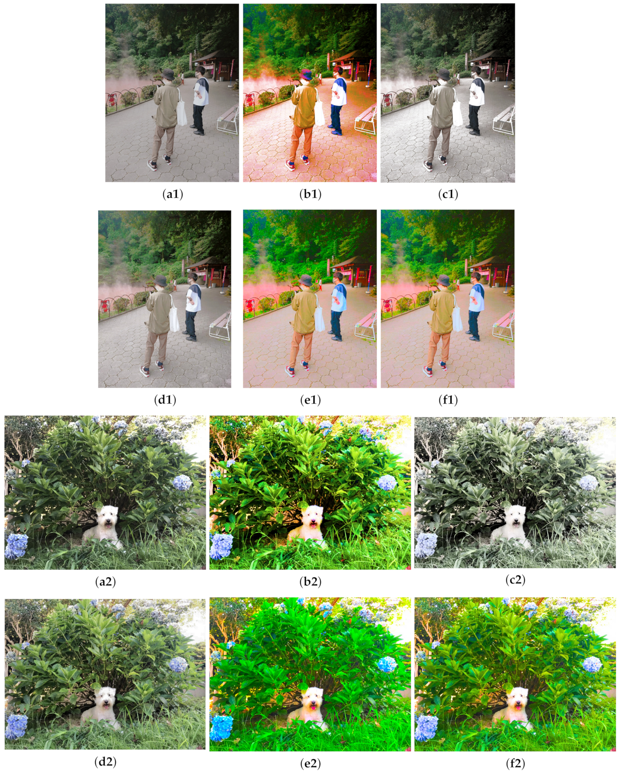
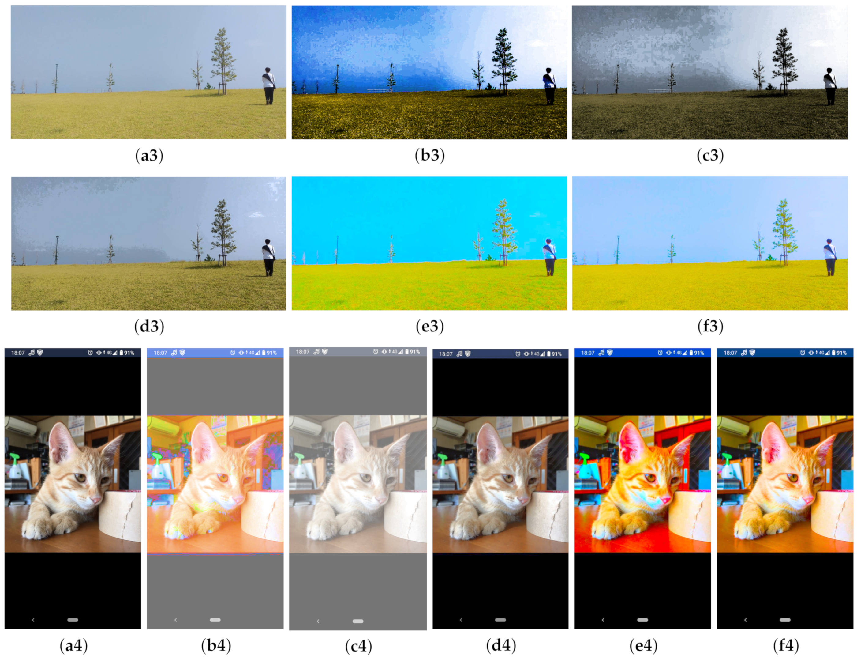
Figure A2 show the experimental results of four digital images. These are 24-bit color images of 960 × 1280 pixels, 1478 × 1108 pixels and 1280 × 622 pixels, 623 × 1280 pixels in size, respectively. We can see that Figure A2e1–e4 are more naturally enhanced in comparison to Figure A2b1,c1,d1,b2,c2,d2 and Figure A2b3,c3,d3,b4,c4,d4. Especially, the colors of the cat and various objects in Figure A2e4 are well reproduced.
5.3. Computational Load
Our previous method is computationally expensive. In contrast, the computational costs of the proposed method are low because it uses the lookup table. The flow of the proposed method is as follows:
- Step 1.
- Input image is converted to the CIELAB color space.
- Step 2.
- Step 3.
- Enhanced image is converted to the RGB color space.
- Step 4.
- If the pixels in the enhanced image are outside the color gamut of the RGB color space, the color gamut adjustment is executed by the lookup table.
6. Conclusions
In this study, we proposed a method of chroma enhancement in the CIELAB color space, which incorporates a lookup table and compared it with that in the RGB color space. The lookup table was implemented to solve the color gamut problem that occurs when inversely converting the CIELAB color space to the RGB color space at low computational costs. The experimental results showed that the proposed method using the CIELAB color space provides better results than that of the RGB color space, especially when performing both the lightness and chroma enhancement.
However, since the methods using the RGB color space does not require the color space conversion, the formulation for image enhancement can be easily realized in comparison to those using the HSI or the CIELAB color space. Furthermore, the color gamut problem does not occur when image enhancement is performed in the RGB color space.
Therefore, the proposed method needs to be further improved its performance. The CIELAB color space is not a complete uniform color space. This limits the performance of the proposed method. Hence, it is expected to extend the proposed method by considering better uniform color spaces that accurately simulate human vision such as DIN99d [32] and CAM02-UCS [33].
Future works are needed to confirm the validity of the images resulting from the proposed method via psychometric assessment and to further improve the quality of enhanced images by refining the accuracy of the maximum chroma assignment by the lookup table [34].
Author Contributions
Conceptualization: N.S.; Methodology: T.A. Both authors contributed equally to this article. All authors have read and agreed to the published version of the manuscript.
Funding
This research received no external funding.
Conflicts of Interest
The authors declare no conflict of interest.
Appendix A
Figure A1.
Experimental results: (1) Pepper, (2) Mandrill, (3) Sailboat, (4) Airplane, (5) Balloon, (6) Earth, and (7) Lenna. (a1–a7) Original images. Output images by (b1–b7) chroma enhancement (RGB, ), (c1–c7) chroma enhancement (CIELAB, ), (d1–d7) chroma enhancement (CIELAB, ) and color gamut adjustment by our previous method, and (e1–e7) chroma enhancement (CIELAB, ) and color gamut adjustment by the lookup table.

Figure A2.
Experimental results. (a1,a2) Original images. Output images by (b1,b2) chroma and lightness enhancement (RGB, , histogram equalization), (c1,c2) the method of Ref. [5] using histogram equalization, (d1,d2) the method of Ref. [7] using default parameters, (e1,e2) chroma and lightness enhancement (CIELAB, , ), and (f1,f2) chroma and lightness enhancement (CIELAB, , ) and color gamut adjustment by the lookup table. (a3,a4) Original images. Output images by (b3,b4) chroma and lightness enhancement (RGB, , histogram equalization), (c3,c4) the method of Ref. [5] using histogram equalization, (d3,d4) the method of Ref. [7] using default parameters, (e3,e4) chroma and lightness enhancement (CIELAB, , ), and (f3,f4) chroma and lightness enhancement (CIELAB, , ) and color gamut adjustment by the lookup table.


Table A1.
Averages and standard deviations of , , and in Figure A1.
Table A1.
Averages and standard deviations of , , and in Figure A1.
| ave | std | ave | std | ave | std | |
|---|---|---|---|---|---|---|
| (b1) | 3.836 | 2.142 | 0.000 | 0.000 | 33.040 | 14.823 |
| (c1) | 12.645 | 9.664 | 7.953 | 8.203 | 46.223 | 13.035 |
| (d1) | 0.224 | 0.699 | 0.029 | 0.171 | 23.940 | 16.369 |
| (e1) | 0.016 | 0.150 | 0.031 | 0.227 | 22.802 | 16.691 |
| (b2) | 1.349 | 1.210 | 0.000 | 0.000 | 32.049 | 17.907 |
| (c2) | 6.763 | 7.433 | 0.950 | 3.491 | 35.602 | 15.934 |
| (d2) | 0.017 | 0.129 | 0.003 | 0.026 | 28.585 | 14.542 |
| (e2) | 0.009 | 0.100 | 0.003 | 0.021 | 27.829 | 14.601 |
| (b3) | 2.350 | 2.724 | 0.000 | 0.000 | 36.777 | 10.661 |
| (c3) | 5.869 | 6.632 | 6.946 | 8.626 | 43.621 | 14.031 |
| (d3) | 0.163 | 0.502 | 0.002 | 0.003 | 29.880 | 12.455 |
| (e3) | 0.036 | 0.212 | 0.003 | 0.010 | 28.774 | 13.066 |
| (b4) | 0.421 | 0.836 | 0.000 | 0.000 | 24.535 | 10.445 |
| (c4) | 0.913 | 2.524 | 0.845 | 4.031 | 24.933 | 24.783 |
| (d4) | 0.003 | 0.020 | 0.004 | 0.009 | 21.153 | 19.274 |
| (e4) | 0.003 | 0.002 | 0.004 | 0.003 | 20.450 | 18.558 |
| (b5) | 0.856 | 0.951 | 0.000 | 0.000 | 33.384 | 14.116 |
| (c5) | 2.559 | 6.620 | 0.514 | 1.378 | 40.062 | 18.335 |
| (d5) | 0.003 | 0.016 | 0.002 | 0.003 | 36.953 | 17.623 |
| (e5) | 0.002 | 0.008 | 0.002 | 0.003 | 36.611 | 17.439 |
| (b6) | 1.058 | 0.681 | 0.000 | 0.000 | 34.598 | 14.955 |
| (c6) | 1.907 | 1.264 | 8.704 | 14.991 | 72.097 | 14.419 |
| (d6) | 0.003 | 0.001 | 0.003 | 0.002 | 49.015 | 25.670 |
| (e6) | 0.004 | 0.001 | 0.003 | 0.002 | 46.926 | 25.850 |
| (b7) | 0.513 | 0.347 | 0.000 | 0.000 | 19.756 | 13.775 |
| (c7) | 10.679 | 6.936 | 4.055 | 14.988 | 54.951 | 9.873 |
| (d7) | 0.005 | 0.003 | 0.000 | 0.002 | 26.863 | 13.405 |
| (e7) | 0.003 | 0.001 | 0.000 | 0.001 | 25.313 | 13.703 |
Table A2.
Averages and standard deviations of , , and in Figure A2.
Table A2.
Averages and standard deviations of , , and in Figure A2.
| ave | std | ave | std | ave | std | |
|---|---|---|---|---|---|---|
| (b1) | 0.991 | 1.140 | 1.990 | 6.494 | 24.768 | 17.487 |
| (c1) | 0.024 | 0.070 | 2.720 | 6.483 | −1.247 | 2.203 |
| (d1) | 0.169 | 0.626 | 4.842 | 5.171 | 3.603 | 5.657 |
| (e1) | 0.841 | 2.081 | 11.429 | 2.931 | 24.765 | 16.642 |
| (f1) | 0.007 | 0.064 | 11.296 | 2.309 | 22.811 | 14.573 |
| (b2) | 1.967 | 1.231 | 2.273 | 8.386 | 33.528 | 17.005 |
| (c2) | 0.131 | 0.174 | 3.970 | 8.482 | −5.353 | 4.661 |
| (d2) | 0.154 | 0.458 | 3.755 | 3.947 | 3.650 | 3.324 |
| (e2) | 4.241 | 5.695 | 12.212 | 4.610 | 46.189 | 20.786 |
| (f2) | 0.005 | 0.038 | 11.609 | 3.903 | 38.464 | 19.173 |
| (b3) | 0.717 | 0.693 | −14.627 | 19.233 | 14.353 | 13.810 |
| (c3) | 0.003 | 0.006 | −14.054 | 18.193 | −4.951 | 5.504 |
| (d3) | 0.065 | 0.135 | −3.700 | 3.629 | 1.301 | 1.067 |
| (e3) | 13.015 | 5.495 | 7.550 | 2.904 | 31.514 | 5.773 |
| (f3) | 0.002 | 0.004 | 8.653 | 1.536 | 20.922 | 11.502 |
| (b4) | 0.114 | 0.258 | 44.572 | 29.079 | 5.865 | 10.769 |
| (c4) | 0.095 | 0.257 | 44.666 | 29.078 | −4.196 | 6.154 |
| (d4) | 0.043 | 0.531 | 2.923 | 4.038 | 0.680 | 2.680 |
| (e4) | 2.505 | 5.296 | 5.317 | 6.734 | 21.035 | 25.491 |
| (f4) | 0.007 | 0.094 | 5.429 | 5.989 | 14.285 | 18.111 |
References
- Hsu, E.; Mertens, T.; Paris, S.; Avidan, S.; Durand, F. Light mixture estimation for spatially varying white balance. ACM Trans. Graph. 2008, 27, 1–7. [Google Scholar] [CrossRef] [Green Version]
- He, K.; Sun, J.; Tang, X. Single image haze removal using dark channel prior. IEEE Trans. Patt. Anal. Mach. Intell. 2011, 33, 2341–2353. [Google Scholar]
- Asmare, M.H.; Asirvadam, V.S.; Iznita, L. Color space selection for color image enhancement applications. In Proceedings of the International Conference on Signal Acquisition and Processing (ICSAP 2009), Kuala Lumpur, Malaysia, 3–5 April 2009; pp. 208–212. [Google Scholar]
- Hunt, R.W.G.; Pointer, M.R. Measuring Colour, 4th ed.; Wiley: Chichester, UK, 2013; p. 159. [Google Scholar]
- Naik, S.K.; Murthy, C.A. Hue-preserving color image enhancement without gamut problem. IEEE Trans. Image Process. 2003, 12, 1591–1598. [Google Scholar] [CrossRef]
- Yang, S.; Lee, B. Hue-preserving gamut mapping with high saturation. Electron. Lett. 2013, 49, 1221–1222. [Google Scholar] [CrossRef]
- Nikolova, M.; Steidl, G. Fast hue and range preserving histogram specification: Theory and new algorithms for color image enhancement. IEEE Trans. Image Process. 2014, 23, 4087–4100. [Google Scholar] [CrossRef] [Green Version]
- Pierre, F.; Aujol, J.-F.; Bugeau, A.; Ta, V.-T. Luminance-hue specification in the RGB Space. In Scale Space and Variational Methods in Computer Vision (SSVM); Springer: Berlin, Germany, 2015; pp. 413–424. [Google Scholar]
- Fitschen, J.H.; Nikolova, M.; Pierre, F.; Steidl, G. A variational model for color assignment. In Scale Space and Variational Methods in Computer Vision (SSVM); Springer: Berlin, Germany, 2015; pp. 437–448. [Google Scholar]
- Pierre, F.; Aujol, J.-F.; Bugeau, A.; Steidl, G.; Ta, V.-T. Hue-preserving perceptual contrast enhancement. In Proceedings of the International Conference on Image Processing (ICIP 2016), Phoenix, AZ, USA, 25–28 September 2016; pp. 4067–4071. [Google Scholar]
- Azetsu, T.; Ueda, C.; Suetake, N.; Uchino, E. Color image enhancement by saturation adjustment while preserving hue in RGB color space. J. Inst. Image Inf. Telev. Eng. 2014, 68, J482–J487. (In Japanese) [Google Scholar]
- Ueda, C.; Ibata, M.; Azetsu, T.; Suetake, N.; Uchino, E. Food image enhancement by adjusting intensity and saturation in RGB color space. IEICE Trans. Fundam. 2015, E98-A, 2220–2228. [Google Scholar] [CrossRef]
- Kamiyama, M.; Taguchi, A. Hue-preserving color image processing with a high arbitrariness in RGB color space. IEICE Trans. Fundam. 2017, E100-A, 2256–2265. [Google Scholar] [CrossRef]
- Pitas, I.; Kiniklis, P. Multichannel techniques in color image enhancement and modeling. IEEE Trans. Image Process. 1996, 5, 168–171. [Google Scholar] [CrossRef] [PubMed]
- Bassiou, N.; Kotropoulos, C. Color image histogram equalization by absolute discounting back off. Comput. Vis. Image Underst. 2007, 107, 108–122. [Google Scholar] [CrossRef]
- Chien, C.L.; Tseng, D.C. Color image enhancement with exact HSI color model. Int. J. Innov. Comput. Inf. Control 2011, 7, 6691–6710. [Google Scholar]
- Yoshinari, K.; Murahira, K.; Hoshi, Y.; Taguchi, A. Color image enhancement in improved HSI color space. In Proceedings of the 2013 International Symposium on Intelligent Signal Processing and Communication Systems (ISPACS 2013), Naha-shi, Japan, 12–15 November 2013; pp. 429–434. [Google Scholar]
- Taguchi, A.; Hoshi, Y. Color image enhancement in HSI color space without gamut problem. IEICE Trans. Fundam. 2015, E98-A, 792–795. [Google Scholar] [CrossRef]
- Fairchild, M.D.; Pirrotta, E. Predicting the lightness of chromatic object colors using CIELAB. Color Res. Appl. 1991, 16, 385–393. [Google Scholar] [CrossRef]
- Tanaka, G. Chroma enhancement method considering effect of lightness and hue. IEICE Tech. Rep. 2012, 112, 19–22. (In Japanese) [Google Scholar]
- Ueda, C.; Azetsu, T.; Suetake, N.; Uchino, E. Color transfer method preserving perceived lightness. Opt. Rev. 2016, 23, 470–478. [Google Scholar] [CrossRef]
- Azetsu, T.; Suetake, N. Hue-preserving image enhancement in CIELAB color space considering color gamut. Opt. Rev. 2019, 26, 283–294. [Google Scholar] [CrossRef]
- Fuentes, S.; Viejo, C.G.; Chauhan, S.S.; Joy, A.; Tongson, E.; Dunshea, F.R. Non-invasive sheep biometrics obtained by computer vision algorithms and machine learning modeling using integrated visible/infrared thermal cameras. Sensors 2020, 20, 6334. [Google Scholar] [CrossRef]
- Cugmas, B.; Sˇtruc, E. Accuracy of an affordable smartphone-based teledermoscopy system for color measurements in canine skin. Sensors 2020, 20, 6234. [Google Scholar] [CrossRef] [PubMed]
- Simko, I. Predictive modeling of a leaf conceptual midpoint quasi-color (CMQ) using an artificial neural network. Sensors 2020, 20, 3938. [Google Scholar] [CrossRef] [PubMed]
- Pitas, I. Digital Image Processing Algorithms and Applications; Wiley-Interscience: New York, NY, USA, 2000; pp. 31–34. [Google Scholar]
- IEC 61966-2-1. Multimedia Systems and Equipment—Colour Measurement and Management—Part2-1: Colour Management—Default RGB Colour Space—sRGB. 1999. Available online: https://webstore.iec.ch/publication/6169 (accessed on 15 March 2021).
- Fairchild, M.D. Color Appearance Models, 3rd ed.; Wiley: Chichester, UK, 2013; p. 201. [Google Scholar]
- The Standard Image Data-BAse (SIDBA). Available online: http://www.ess.ic.kanagawa-it.ac.jp/app_images_j.html (accessed on 15 March 2021).
- CIE Publication. “Colorimetry”, No.15; CIE Central Bureau: Vienna, Austria, 2004. [Google Scholar]
- Ha¨user, S.; Steidl, G.; Nikolova, M. Hue and Range Preserving RGB Image Enhancement (RGB-HP-ENHANCE), Preprint. 2015. Available online: http://www.mathematik.uni-kl.de/imagepro/forschung/software/rgb-hp-enhance/ (accessed on 15 March 2021).
- Cui, G.; Luo, M.R.; Rigg, B.; Roesler, G.; Witt, K. Uniform colour spaces based on the DIN99 colour-difference formula. Color Res. Appl. 2002, 27, 282–290. [Google Scholar] [CrossRef]
- Luo, M.R.; Cui, G.; Li, C. Uniform colour spaces based on CIECAMO2 colour appearance model. Color Res. Appl. 2006, 31, 320–330. [Google Scholar] [CrossRef]
- Villecco, F. On the evaluation of errors in the virtual design of mechanical systems. Machines 2018, 6, 36. [Google Scholar] [CrossRef] [Green Version]
Figure 1.
Straight line J satisfying equal hue and equal lightness in RGB color space, and chroma S of each color on J.
Figure 1.
Straight line J satisfying equal hue and equal lightness in RGB color space, and chroma S of each color on J.

Figure 3.
Lookup table plotted with contour lines. n, hue; m, lightness.

Figure 4.
Assignment of maximum chroma value using lookup table.

Publisher’s Note: MDPI stays neutral with regard to jurisdictional claims in published maps and institutional affiliations. |
© 2021 by the authors. Licensee MDPI, Basel, Switzerland. This article is an open access article distributed under the terms and conditions of the Creative Commons Attribution (CC BY) license (https://creativecommons.org/licenses/by/4.0/).
Share and Cite
MDPI and ACS Style
Azetsu, T.; Suetake, N. Chroma Enhancement in CIELAB Color Space Using a Lookup Table. Designs 2021, 5, 32. https://0-doi-org.brum.beds.ac.uk/10.3390/designs5020032
AMA Style
Azetsu T, Suetake N. Chroma Enhancement in CIELAB Color Space Using a Lookup Table. Designs. 2021; 5(2):32. https://0-doi-org.brum.beds.ac.uk/10.3390/designs5020032
Chicago/Turabian StyleAzetsu, Tadahiro, and Noriaki Suetake. 2021. "Chroma Enhancement in CIELAB Color Space Using a Lookup Table" Designs 5, no. 2: 32. https://0-doi-org.brum.beds.ac.uk/10.3390/designs5020032