Drone Laser Scanning for Modeling Riverscape Topography and Vegetation: Comparison with Traditional Aerial Lidar


1
Department of Geographical Sciences, University of Maryland, College Park, MD 20740, USA
2
Department of Biological Systems Engineering, Virginia Tech, Blacksburg, VA 24060, USA
*
Author to whom correspondence should be addressed.
Drones 2019, 3(2), 35; https://0-doi-org.brum.beds.ac.uk/10.3390/drones3020035
Submission received: 8 March 2019
/
Revised: 9 April 2019
/
Accepted: 10 April 2019
/
Published: 12 April 2019
Abstract
:Lidar remote sensing has been used to survey stream channel and floodplain topography for decades. However, traditional platforms, such as aerial laser scanning (ALS) from an airplane, have limitations including flight altitude and scan angle that prevent the scanner from collecting a complete survey of the riverscape. Drone laser scanning (DLS) or unmanned aerial vehicle (UAV)-based lidar offer ways to scan riverscapes with many potential advantages over ALS. We compared point clouds and lidar data products generated with both DLS and ALS for a small gravel-bed stream, Stroubles Creek, located in Blacksburg, VA. Lidar data points were classified as ground and vegetation, and then rasterized to produce digital terrain models (DTMs) representing the topography and canopy height models (CHMs) representing the vegetation. The results highlighted that the lower-altitude, higher-resolution DLS data were more capable than ALS of providing details of the channel profile as well as detecting small vegetation on the floodplain. The greater detail gained with DLS will provide fluvial researchers with better estimates of the physical properties of riverscape topography and vegetation.
1. Introduction
Riverscapes are complex, interconnected ecosystems consisting of channels, banks, riparian zones, and floodplains [1]. Biotic communities and ecosystem processes are strongly responsive to the physical aspects of riverscapes. The quantification of these physical properties depends on time- and space-varying parameters, such as inundated surface area, riparian structure, streambed habitat complexity, and turbulence within the water column, as well as at the sediment–water and water–air interfaces. Riverscapes are difficult to quantify, particularly when considering their continuous, heterogeneous characteristics over time and space [2]. Some studies represent riverscape habitat complexity through the spatial variability of the environment. This variability can be defined by various metrics including topographic roughness [3], hydraulic roughness [4], topographic complexity [5], or hydraulic complexity [6].
To study riverscape complexity, both the topography and vegetation must be considered [7]. Topographic complexity is defined by channel shape using metrics such as the degree of meandering [7], or channel surface material using measures such as grain-size distribution [8]. Vegetative complexity, an important measure for ecological engineering applications such as stream restoration [9], is typically estimated through roughness parameters (e.g., Manning’s roughness coefficient) and vegetation density [10]. While the methods for measuring these metrics have a long history in fluvial studies, they tend to be coarsely measured (e.g., pebble counts for grain-size distribution [11]), visually estimated (e.g., in-stream cover [6]), or require intensive model calibration (e.g., hydraulic roughness [12]). Uncertainties resulting from these measurements can propagate through to final project outcomes and modeling results. Resop et al. [13] found that the channel dimensions (width and depth) for a two-stage stream restoration design were sensitive to the estimated value for the Manning’s roughness coefficient, particularly when estimating floodplain discharge.
Recent advances in photogrammetric techniques such as structure-from-motion (SfM), the availability of terrestrial and aerial laser scanning, and use of unmanned aerial vehicles (UAVs; i.e., drones) has led to heightened interest in applying these technologies to hydrological and biological studies. Aerial-based lidar or aerial laser scanning (ALS; from airplanes or helicopters) has been used in many ecological studies of riverscapes for measuring topography. Clubb et al. [14] delineated floodplain areas from ALS-derived 1-m digital terrain models (DTMs). McKean et al. [15] measured stream geometry and cross-sectional area using a bathymetric ALS with DTM resolutions between 1 to 3 m. However, ALS is usually limited to point densities less than 10 points/m2. While this is a high resolution for many applications, it is inadequate for quantifying micro-changes in terrain, which are important for measures of grain-size and roughness [16]. Another concern with ALS is that it is difficult to scan the sides of shear surfaces such as cliffs and vertical or undercut banks due to the altitude and scan angle of the aircraft [15,17]. These limitations are an issue when measuring stream topographies, particularly for small streams, since streambanks are insufficiently profiled with ALS.
Ground-based lidar or terrestrial laser scanning (TLS) offers improved point densities (greater than 1000 points/m2) because the lidar systems are set on tripods, and thus, much closer to the target surface. Terrestrial laser scanning also acquires higher point densities than ALS on the sides of streambanks due to a more direct scan angle [18]. Like ALS, TLS has been used in many studies to measure riverscapes. Heritage and Hetherington [16] used TLS to scan a 150-m stream reach at 0.01-m resolution with 21 scans from different locations and angles over the riverscape. Heritage and Milan [8] demonstrated a relationship between streambed grain size and the standard deviation of TLS point elevations within a 0.15-m moving window. Resop et al. [18] measured streambank retreat for an 11-m bank of Stroubles Creek in Blacksburg, VA over two years using TLS-derived 0.02-m DTMs. In another study, Resop et al. [5] quantified habitat complexity in a forested, 100-m stream reach using 89 TLS scans based on the size and location of in-stream boulders from a 0.02-m DTM. While TLS has a much higher resolution than ALS, it is limited by mobility and extent. Data gaps can also result from TLS scans due to the shadowing effect caused by large features obstructing the laser [5,16]. Mobile laser scanning (MLS) systems attached to ground vehicles have the potential to scan larger areas than TLS, but are not practical for the rough, densely vegetative terrain that typically defines riverscapes or they are limited to measurements from within the waterbody itself [19].
Initial research with drone-based remote sensing for studying riverscapes has focused primarily on imagery data using SfM techniques [20]. Dandois and Ellis [21] developed the computational pipeline Ecosynth to processes drone-based imagery, produce 3-D point clouds of forested environments, and estimate canopy height models (CHMs) comparable to results produced from ALS. Woodget et al. [22] used drone-based imagery to create a 0.02-m DTM of a stream and map the geomorphology, including the classification of topography, grain size, roughness, and vegetation. However, drone-based photogrammetry using SfM is limited to surveying the top of the canopy, while lidar has the advantage of better canopy penetration.
Recently, ultra-light lidar systems have become integrated with UAV systems [23,24,25]. While drones are more limited than ALS surveys in terms of total area of extent, they provide the ability to scan the environment closer to the earth’s surface. Lower altitude scans result in far greater point densities than ALS (greater than 400 points/m2) and improved detail of hard-to-scan features such as vertical streambanks, making drone-based lidar or drone laser scanning (DLS) well suited for surveying the topography of complex riverscapes.
This study utilized DLS and ALS data for a small stream, Stroubles Creek, in Blacksburg, VA. The objectives were to: (1) create tools for automating lidar data processing based on standard ALS data workflows and determine their effectiveness with higher-resolution DLS data; (2) classify points in both datasets and compare their ability to represent riverscape terrain and vegetation; and (3) produce surface models representing terrain (DTMs) and vegetation (CHMs) and compare results between DLS and ALS.
2. Materials and Methods
2.1. Study Area
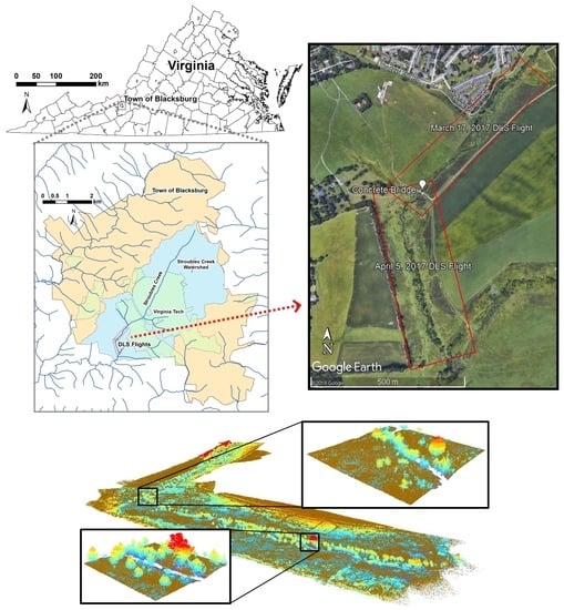
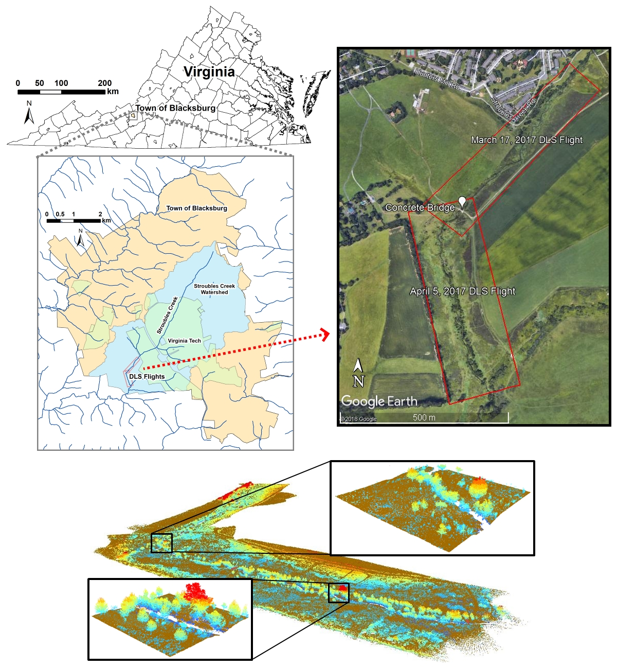
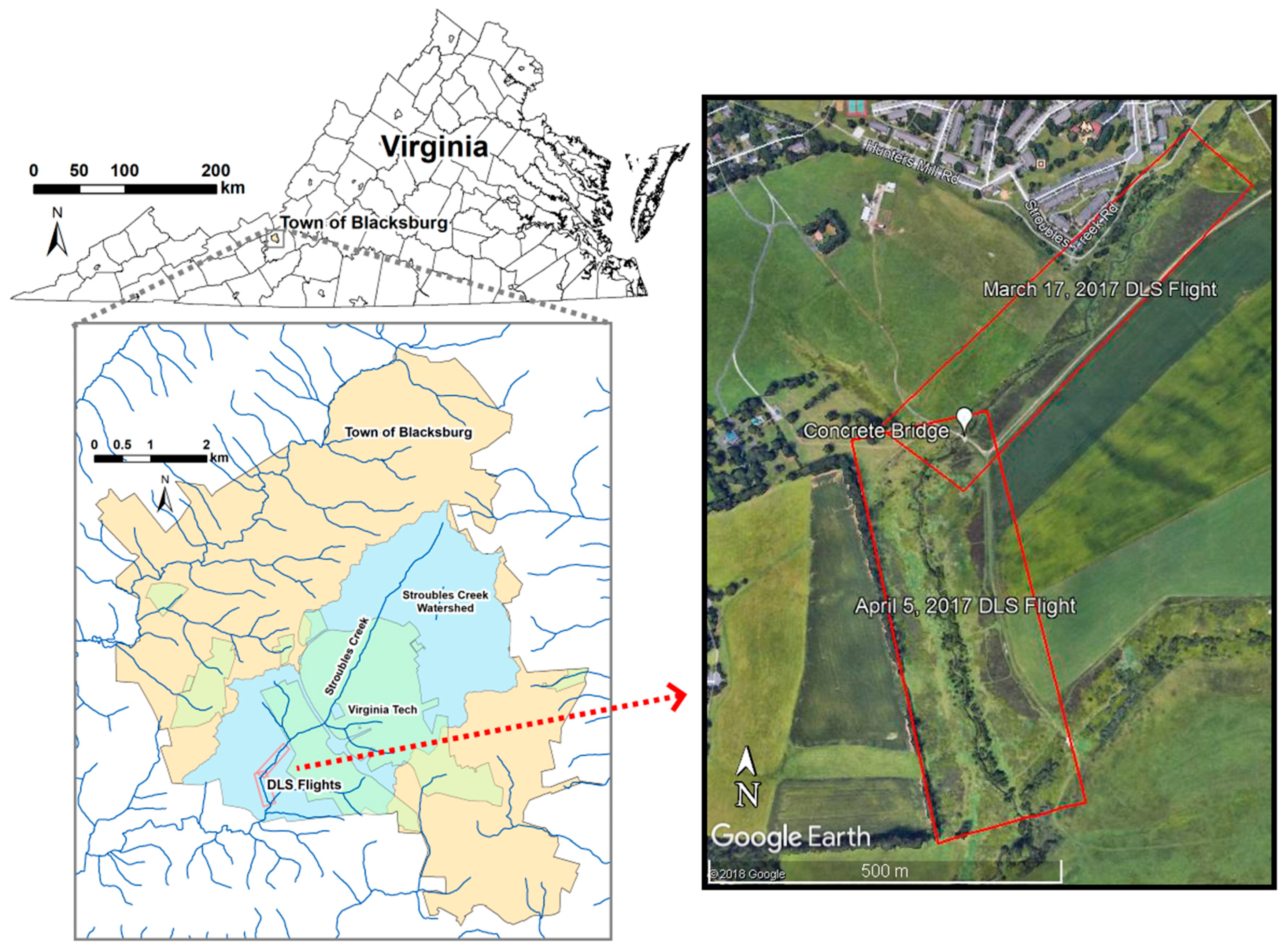
The study area was a 1.3-km reach of Stroubles Creek, a gravel-bed stream downstream of the Virginia Tech campus in Blacksburg, VA (Figure 1). Stroubles Creek is on the Environmental Protection Agency’s 303(d) list of impaired streams due to sediment loading from agricultural and urban sources [26]. A stream restoration for this section of Stroubles Creek was completed in May 2010 [27]. The restoration project consisted of best management practices, such as fencing off livestock from direct stream access, bank reshaping, vegetation replanting, and creating an inset floodplain. Stroubles Creek is continuously monitored for flow, water quality, and weather as part of the Stream Research, Education, and Management (StREAM) Lab at Virginia Tech to determine the effectiveness of the restoration project on water quality and ecological sustainability [28].
2.2. Lidar Data Collection
The DLS system used for this study consisted of a Vapor35 drone (Pulse Aerospace Inc., Lawrence, KS) with an integrated YellowScan Surveyor Core lidar (Montferrier-sur-Lez, France). The Vapor35 UAV uses the weControl SA wePilot1000 flight control system with integrated Global Navigation Satellite System (GNSS) and the weGCS ground control station software for mission planning and execution. The drone has a maximum payload of 2.3 kg and a battery capable of 60 min flight time. The YellowScan lidar is an ultra-light system (2.1 kg), which makes it an ideal payload for the Vapor35. The system uses an Applanix AV39 GNSS antenna paired with the Velodyne (San Jose, CA) lidar puck and onboard computer for self-contained, one-button data acquisition. The lidar system is capable of recording up to two returns per pulse and uses a near-infrared wavelength of 905 nm. Once the data were collected, the GNSS trajectory of the lidar unit was corrected with local National Geodetic Survey CORS base station data and the corrected trajectory was applied to produce point data in the LAS file format.
Two DLS surveys were flown at an altitude of 20 m over Stroubles Creek during the spring season, on 17 March and 5 April 2017 (Figure 2c). The 17 March flight scanned the northern half of the reach, while the 5 April flight scanned the southern half (Figure 1), resulting in 90 million points for the entire reach. Most points were 1st return (98.5%) with the rest being 2nd return.
The data collected with DLS were compared with data from two separate ALS surveys (2010 and 2016). The main purpose of including the ALS datasets was to provide a comparison between the point densities and the amount of detail obtained of the physical riverscape environment between the newer technology of DLS and the more traditional ALS. The 2017 DLS survey was primarily compared with the 2016 ALS dataset for analysis purposes due to the closer proximity of the scanning dates. The 2010 ALS dataset was included mainly to serve as a historical perspective of the evolution of ALS technology and to compare it against current DLS technology. In addition, one can compare the 2010 and 2016 ALS datasets to gain some insight on the changes that have occurred in the riverscape environment since the 2010 stream restoration [27].
On 30 March 2010 (Figure 2a), the Virginia Information Technologies Agency (VITA) performed an aerial survey for the City of Blacksburg using a Leica ALS-50 lidar with a wavelength of 1064 nm and up to four returns recorded per pulse [29]. The survey was flown at an altitude of 1500 m, used a maximum scan angle of ±20°, and included an average swath overlap of 40%. Two point clouds in the LAZ file format representing the study area were downloaded from VITA’s website [30].
From 20–22 December 2016 (Figure 2b), Pictometry International, Inc. scanned Virginia Tech campus using an Optech Galaxy Airborne Laser Terrain Mapper (ALTM), which has a wavelength of 1064 nm and records up to eight returns per pulse. The survey was flown at an altitude of 2500 m with a scan angle of ±15.8°, a swath width of 1400 m, and 30% overlap between swaths. Data covering the study area were downloaded as four LAS files.
2.3. Lidar Data Processing
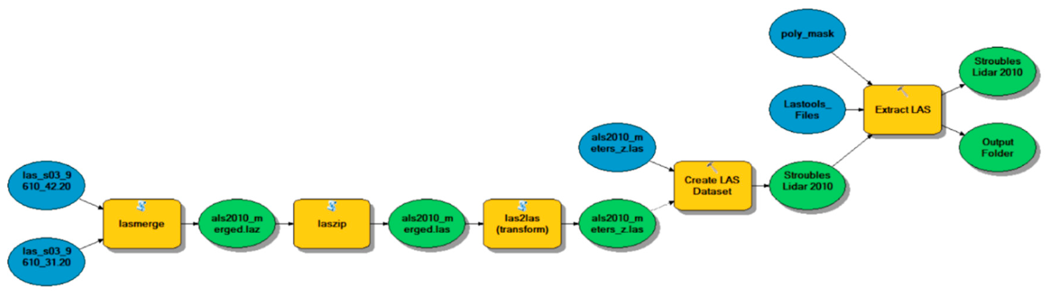
Lidar data processing pipelines for both DLS and ALS were created using ModelBuilder in ArcGIS 10.5 (Redlands, CA) with scripts utilizing tools from ArcGIS and LAStools (Gilching, Germany). The ALS point clouds were combined into a single LAZ file using LASmerge and converted from LAZ to LAS format using LASzip [31] (Figure 3). The Z (elevation) units were converted from feet to meters to be comparable with the DLS dataset using the tool LAS2LAS and a Z scale multiplier of 0.3048. The ALS dataset was then clipped to the extent mask of the DLS survey, derived below, using the “Extract LAS” tool.
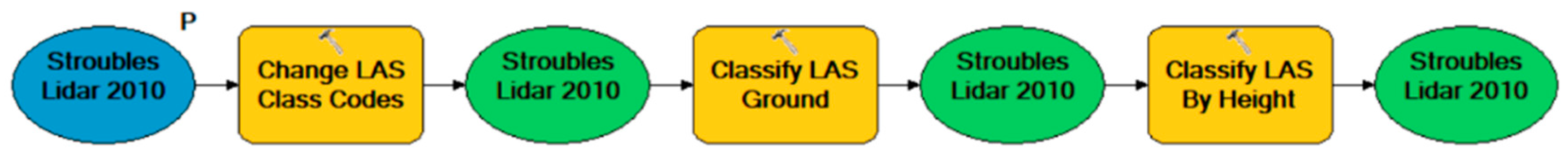
The raw point cloud data collected by DLS were not classified. Before automated classification, the DLS dataset was manually edited to classify obvious outliers (e.g., “bird hits”) as noise. Both ALS surveys were originally classified by the vendor as unassigned, ground, noise, and overlap. Points classified as ground and overlap were reclassified as unassigned using the “Change LAS Class Codes” tool. After the point classification codes for DLS and ALS were pre-processed, they were then classified as ground and vegetation using a similar workflow (described below).
The lidar datasets were classified into LAS class codes of ground and vegetation (Figure 4). The “Classify LAS Ground” was used to first classify points as ground versus unassigned. The “Classify LAS by Height” tool was then used to classify the remaining points as vegetation versus unassigned, using a height range between 0.1 m and 25 m to define vegetation. The unassigned category represented low points with a height less than 0.1 m, which cannot be distinguished between ground and vegetation. Points with a height value below 0 m or above 25 m were classified as noise. A manual classification was performed to classify human-built structures (e.g., bridges, fences, and cars) using the building class code. Finally, the datasets were manually inspected in ArcGIS to correct misclassified points.
The classified lidar datasets were rasterized to produce various digital elevation models (DEMs), including bare earth models (DTMs) and vegetation models (CHMs). Lidar data processing pipelines were again created using ModelBuilder. An extent mask was created to represent the boundary of the DLS survey and clip all subsequent rasters. The “LAS Point Statistics as Raster” tool was used to calculate the point density over a 0.1-m grid. Cells with a point count greater than zero were selected with the “Con” tool and then morphological closing (“Expand” followed by “Shrink”) was used to fill in small gaps in the raster. The raster cells were converted to polygons with the largest resulting polygon representing the areal extent of the DLS survey.
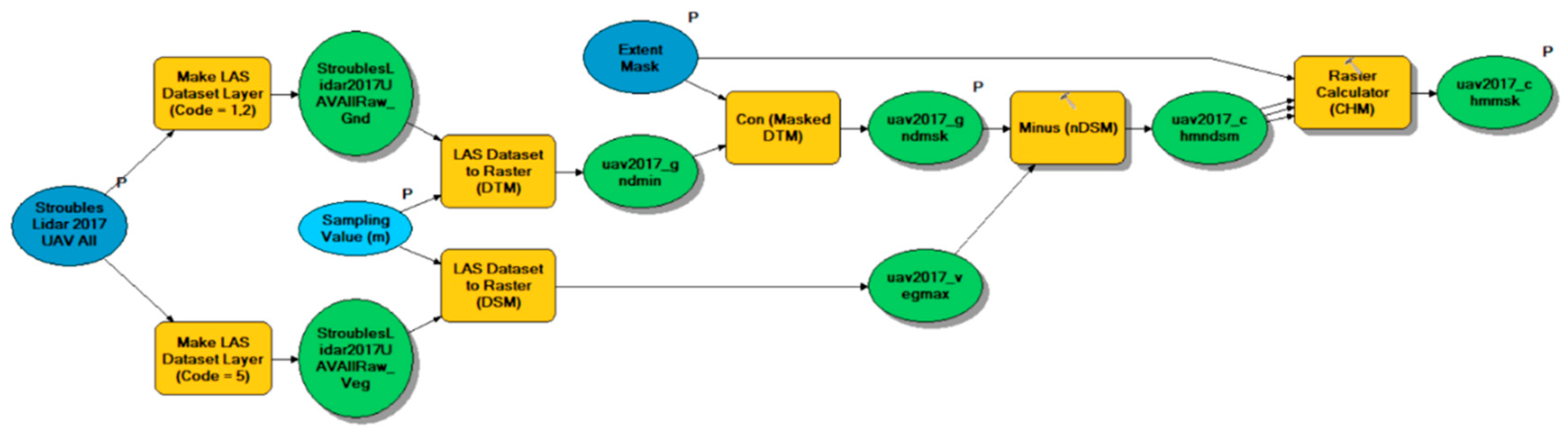
The elevation models (DTMs and CHMs) were created using the “LAS Dataset to Raster” tool (Figure 5). Raster resolution was set to 0.1 m for DLS and 1 m for ALS, based on their average point spacing (0.047 m for DLS, 0.652 m for 2010 ALS, and 0.488 m for 2016 ALS). To create the DTM, only ground and unassigned points were selected. A raster was then created using the minimum lidar point elevation for each cell and simple linear interpolation to fill in small data gaps. To create the CHM, a digital surface model (DSM) was first created by selecting only vegetation points and rasterizing using the maximum lidar point elevation for each cell and no interpolation used for data gaps. A normalized DSM (nDSM) was calculated using map algebra as the DSM minus the DTM, resulting in Z values representing height above ground. Gaps in the nDSM and cells with heights less than 0.1 m were set to zero; the result defined the CHM.
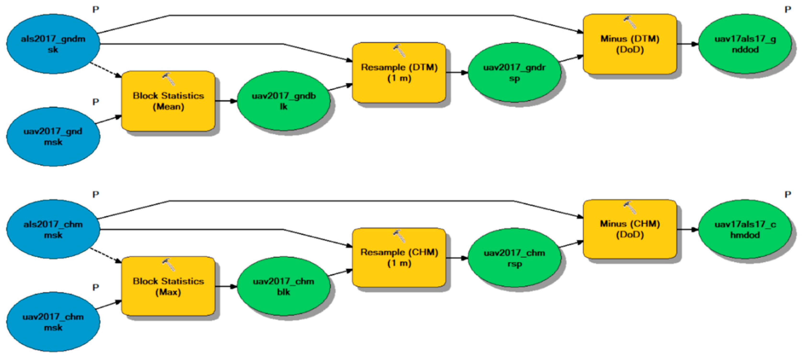
To compare the DTMs and CHMs between DLS and ALS, DEMs of difference (DoDs) were calculated with map algebra by subtracting the ALS DEM from the DLS DEM (Figure 6). To resolve resolution inconsistencies, the 0.1-m DLS rasters were resampled to a 1-m cell size using the “Block Statistics” and “Resample” tools. The DTM was resampled using the mean cell value and the CHM was resampled using the maximum cell value.
3. Results
3.1. Lidar Data Statistics
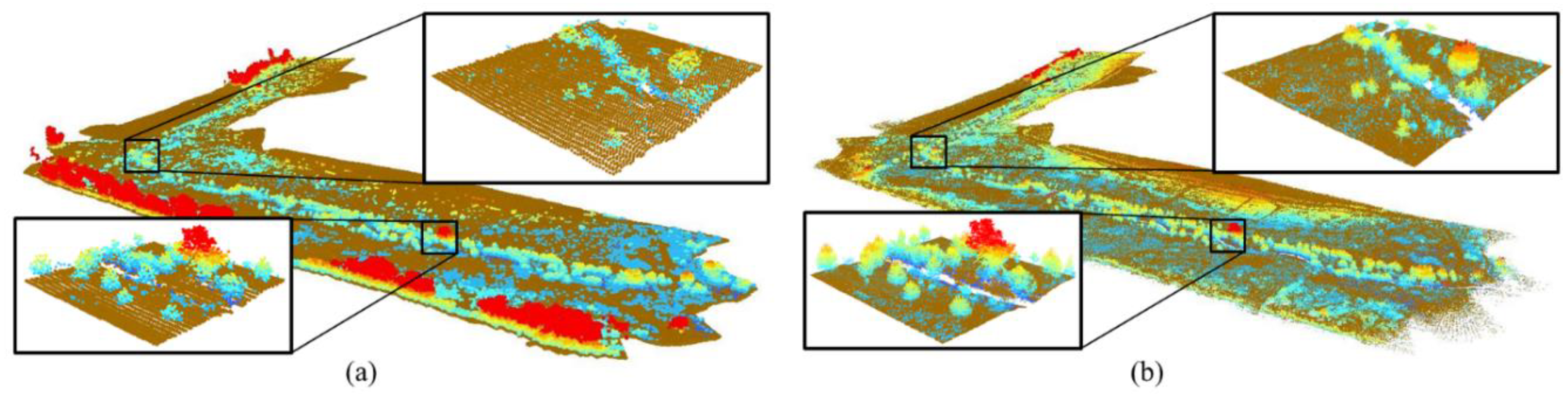
There were many similarities and differences between the ALS and DLS datasets in terms of the raw data statistics. Compared with the 90 million points collected by DLS over the study area, ALS scanned less than a million points for each survey (Table 1). This corresponds to an overall density of 2.35 points/m2 and 4.20 points/m2 for the 2010 ALS and 2016 ALS, respectively, and a much higher density of 455 points/m2 for DLS. This difference was observed in the point clouds, with DLS surveying the riverscape topography and vegetation in much greater detail than ALS (Figure 7). In particular, DLS detected short herbaceous vegetation and small walking paths in the floodplain better than ALS. However, DLS has the same limitation as ALS in that the water surface absorbs near-infrared lidar pulses, resulting in data gaps within the stream channel.
3.2. Classified Lidar Data
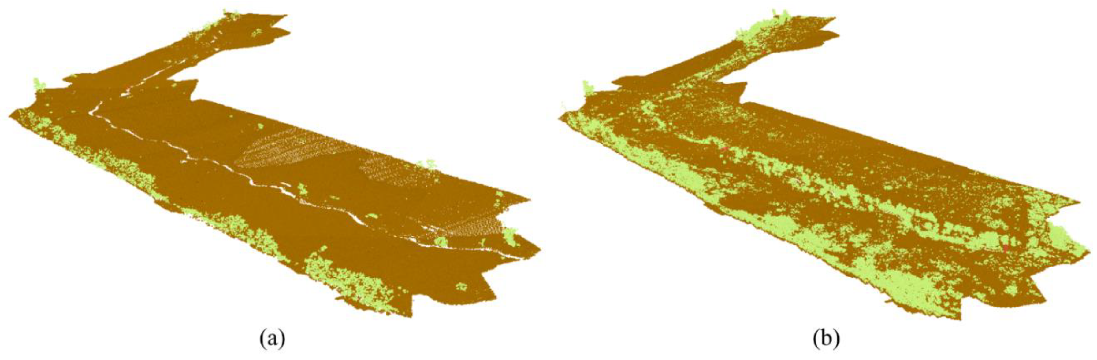
The 2010 ALS dataset consisted of 98% ground and 2% vegetation, while the 2016 ALS dataset consisted of 88% ground and 12% vegetation (Table 1). The difference in vegetation between the 2010 and 2016 ALS datasets (2% versus 12%) was mostly due to changes that have occurred since the 2010 Stroubles Creek restoration project [27]. Much of the increase in vegetation resulted from replanting efforts along the streambank and within the floodplain (Figure 8).
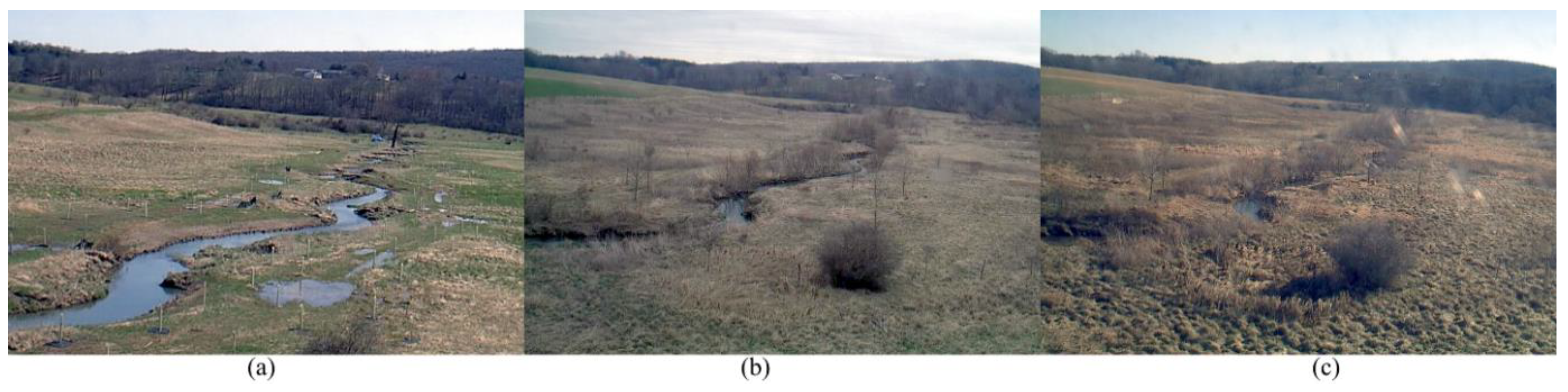
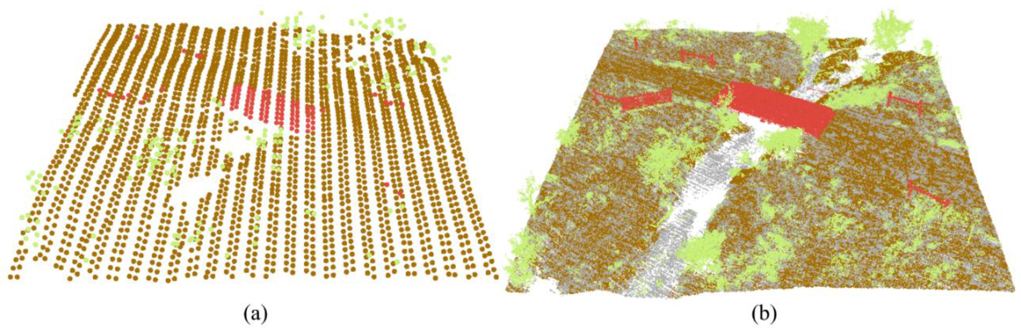
The DLS and 2016 ALS and datasets produced similar percentages of vegetation points, 13% and 12%, respectively (Table 1). There was a three-month time difference between the two datasets (December 2016 for ALS and March/April 2017 for DLS). More similar flight times would have been ideal; however, the timing of the ALS survey was outside of our control. As seen from the StREAM Lab camera tower, these surveys occurred during the same leaf-off dormant vegetation season (Figure 2). The resolution of DLS was capable of capturing more of the grasses and shorter vegetation throughout the floodplain that were missed by ALS (Figure 9). In addition, the concrete bridge in the middle of the reach (Figure 1) as well as other features, such as wooden fences and sample bridges, were detected in much greater detail with DLS than with ALS.
As a quick accuracy assessment, we compared measurements in the field of the concrete bridge and several fence posts (Figure 9) to estimates using lidar point cloud data with ArcGIS (Table 2). For all metrics, DLS was more accurate than ALS. As an example, the width of the concrete bridge (3.57 m in the field) resulted in a relative error of 0.93% using the DLS data and 6.37% using the ALS data. This improved accuracy of DLS over ALS for measuring fine details in the environment could be critical for hydraulic applications where minor obstructions can influence flow or for ecological applications where rocks and woody debris can impact habitat complexity.
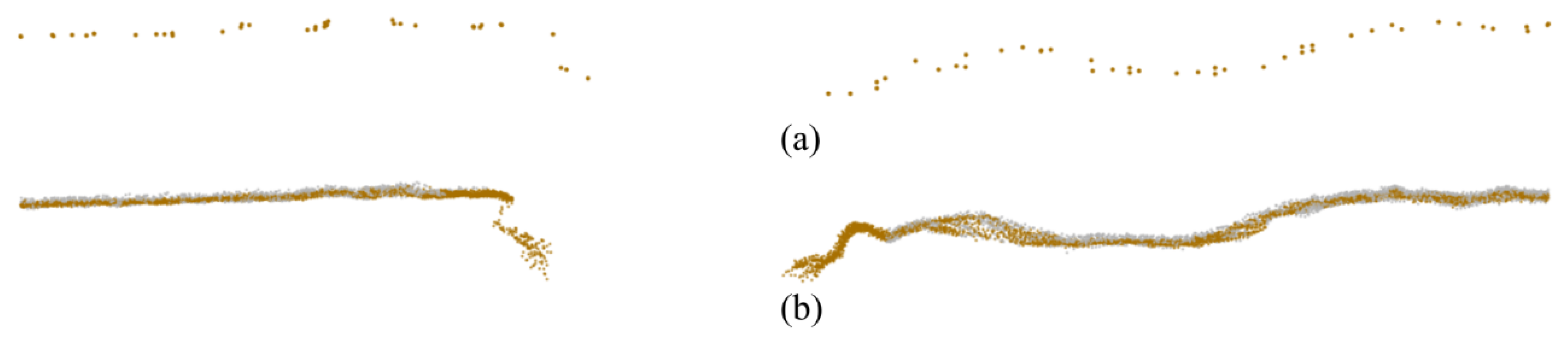
With respect to the terrain, a lower percentage of points were classified as ground with DLS than with the 2016 ALS (53% versus 88%) and the DLS dataset contained a greater percentage of unassigned points compared with ALS (34% versus 0%), which represent points with a height between 0 and 0.1 m. These points represent uncertainty in the terrain and likely represent micro-changes in soil elevation or short vegetation. These points have the potential to represent heterogeneity in the topography and could be used for estimating metrics such as complexity or roughness [8]. Drone laser scanning also performed better than ALS in providing a more complete scan of the streambank profiles, which is critical for quantifying geomorphological change like streambank retreat [18] (Figure 10). Aerial laser scanning, with a lower point density, was unable to detect local variabilities in the terrain. While most points in the ALS dataset were ground, these points were coarsely spaced and only represented the general trend of the topography (Figure 10a). Drone laser scanning captured more of the spatial heterogeneity of the terrain when combining ground and unassigned points (Figure 10b).
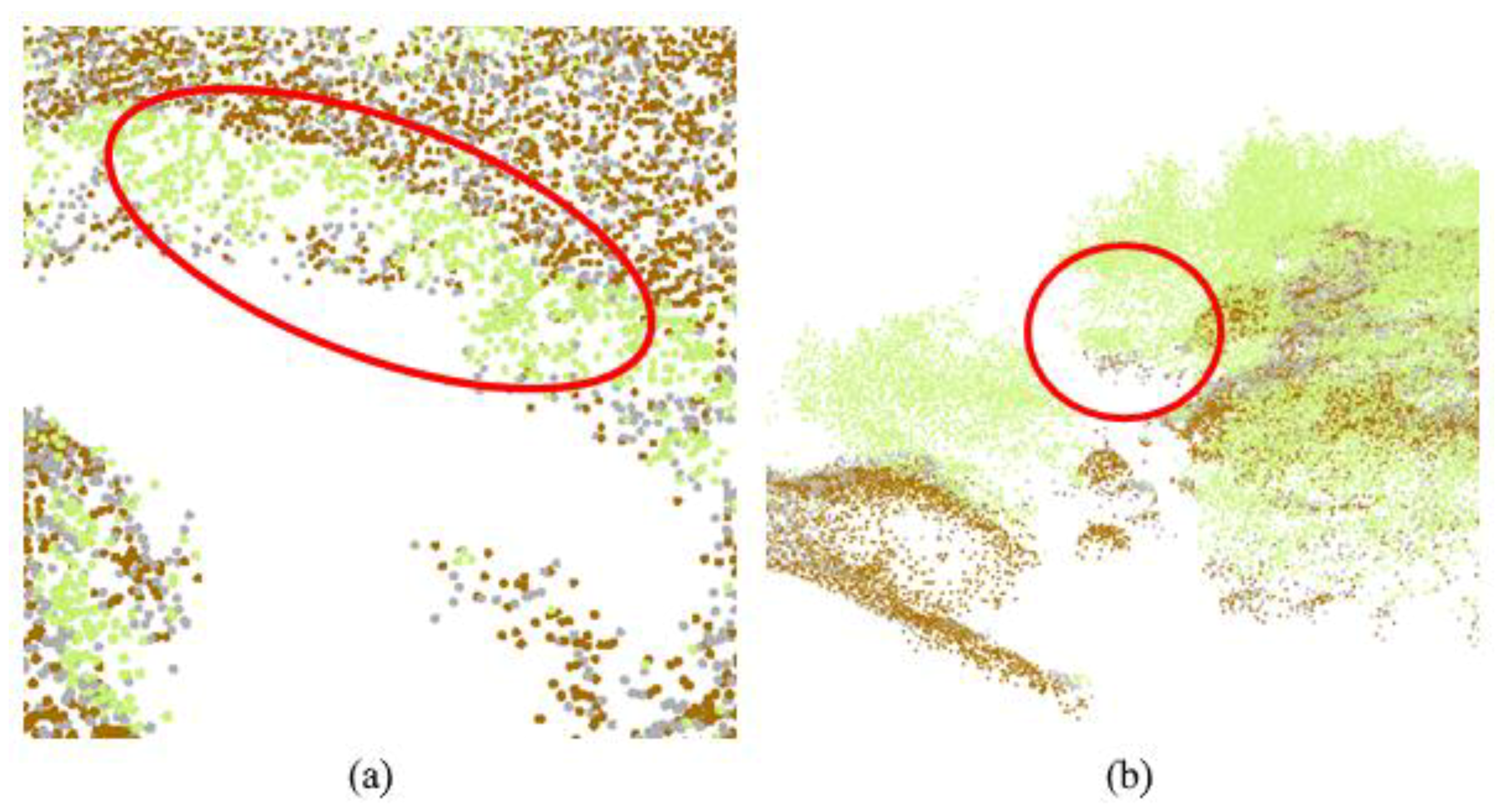
Two common classification errors with DLS were: (1) points misclassified as vegetation; and (2) points misclassified as ground. The first error type occurred along steep streambanks (Figure 11a). Points representing ground were misclassified as unassigned by the “Classify LAS Ground” tool likely because of the sharp gradient of many streambanks and the data gap in the stream channel. A tool parameter, the ground detection method, allows for more aggressive ground classification and is supposed to help in areas with steep ridges, but we did not notice a significant improvement by changing this parameter. Once these points were misclassified as unassigned instead of ground, the “Classify LAS by Height” tool then misclassified them as vegetation. The second error type occurred in dense vegetation overhanging the stream (Figure 11b). In these cases, the lower canopy points were misclassified as ground, again due to the data gap. Both types of misclassification where corrected manually, which was a time-consuming process and not a complete solution.
3.3. Rasterized Lidar Data
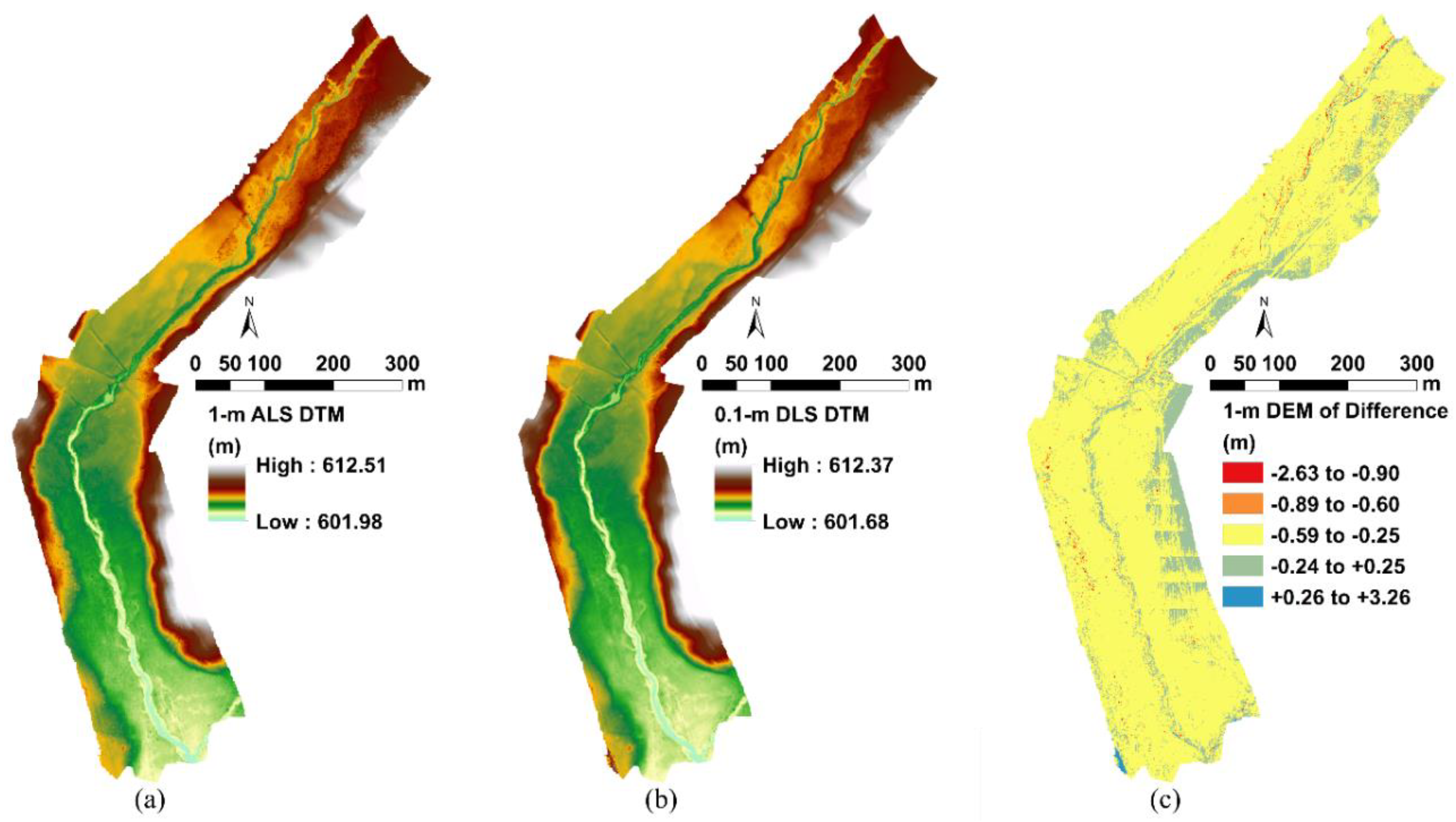
Digital terrain models (DTMs) representing bare earth were generated from the DLS and ALS datasets. Both the 2016 ALS and 2017 DLS models showed similar trends in the topography (Figure 12). However, the DLS DTM provided greater detail of the terrain because of the higher resolution. For example, in the DLS DTM, one can observe small paths, tire tracks on dirt roads, and in-stream features, such as rocks and point bars. The DTMs were subtracted to produce a DoD (Figure 12c). The mean elevation difference between DTMs was −0.322 m. The most probable cause of this bias is from georeferencing errors. It is important to note that when the 2010 ALS and 2016 ALS DTMs were compared (not shown), the mean elevation difference was −0.253 m. There are potentially many sources of error, but these biases are similar to vertical accuracies commonly reported for ALS (0.15 m and higher) [32].
Since the 2016 ALS and 2017 DLS surveys were completed approximately three months apart, most of the change between DTMs was likely not due to topographic change such as erosion or streambank retreat. Instead, much of the difference was likely a result of measurement errors between the lidar platforms. The largest differences occurred within the channel and along banks (Figure 12c). This was likely because ALS could not scan the sides of streambanks effectively, resulting in interpolation errors. It is common for ALS to report greater elevation errors along steeper slopes [32]. Drone laser scanning more precisely scanned the streambanks due to its lower altitude and higher point density, and thus produced in a more representative model of the channel (Figure 10).
A striping pattern was observed in the DTM DoD between the 2016 ALS and 2017 DLS surveys in the lower right section of the study area (Figure 12c). This same striping pattern was also observed in the DoD between the 2010 ALS and 2016 ALS DTMs (not shown). Upon closer inspection of the raw point clouds, the most likely causes for this data artifact were: (1) the flight pattern of the 2016 ALS survey; and (2) minor projection errors during conversion from the projection of the ALS dataset (2011 State Plane Virginia South (feet)) to the projection of the DLS dataset (UTM Zone 17 N (meters)).
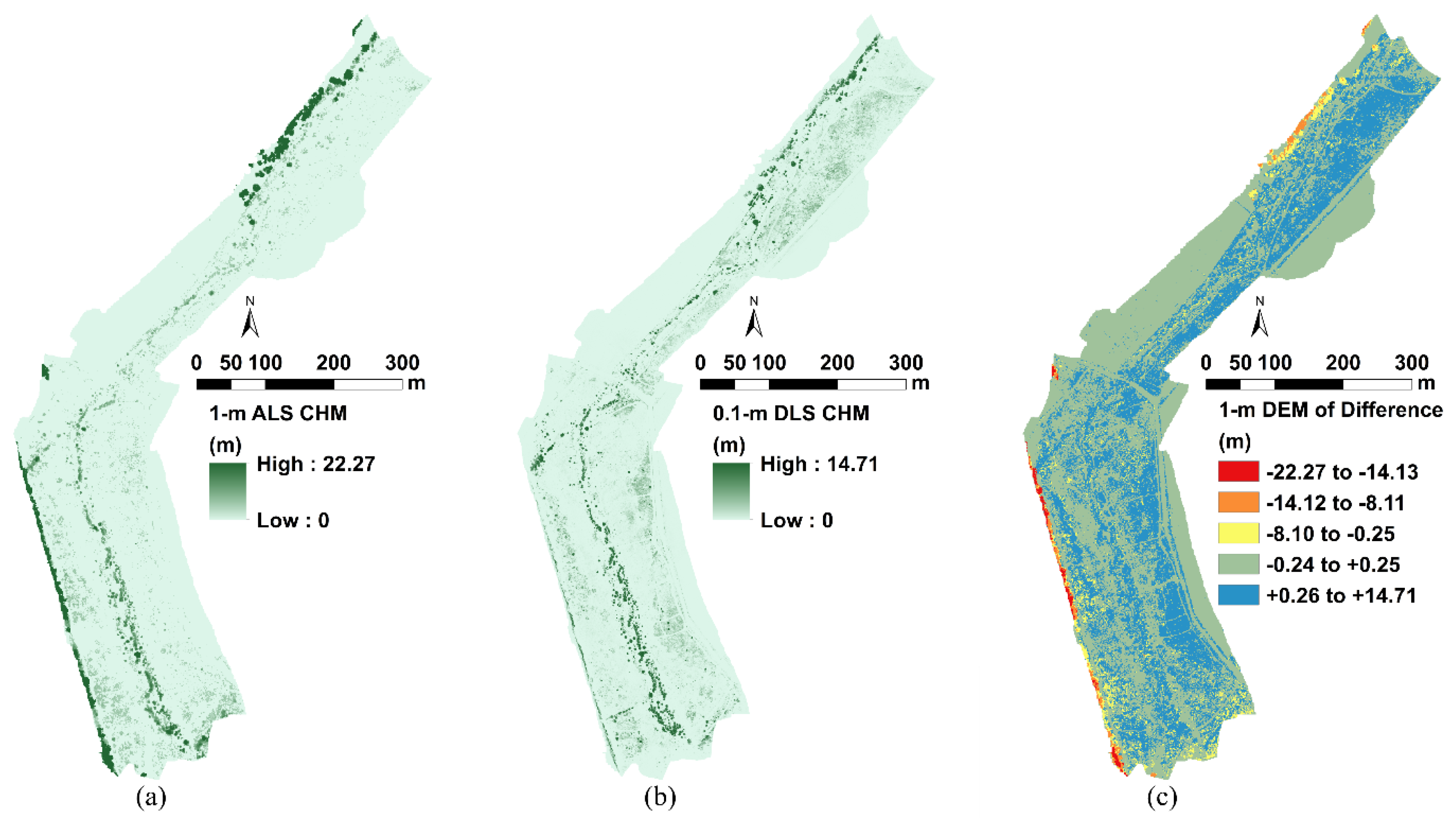
Canopy height models (CHMs) created from the ALS and DLS datasets represented streambank and floodplain vegetation (Figure 13). The only vegetation observed in the 2010 ALS CHM (not shown), which occurred before the stream restoration, were a few scattered trees throughout the floodplain and a row of trees along the southwest boundary. The 2016 ALS CHM represented the vegetation resulting from the restoration project (Figure 13a). Positive values in the DoD between the 2010 and 2016 ALS CHMs provide a measure of the vegetation growth throughout the study area (mean elevation difference of +0.398 m and maximum difference of +22.270 m) resulting from more than six years of vegetation growth since the restoration project.
The higher resolution DLS CHM provided more detail of the tree canopy, small bushes, and tall grasses on the streambanks and floodplains (Figure 13b). A DoD was created by subtracting the 2016 ALS CHM from the 2017 DLS CHM (Figure 13c). Since the Z value of both CHMs were normalized to height above ground, model bias was less of a concern than with the DTMs. The mean height difference was +0.111 m between CHMs. As discussed previously, this difference in vegetation height was likely not due to the growth of grasses and leaves during the three-month difference between the ALS and DLS flights since they both occurred during the same leaf-off dormant vegetation season. Much of this difference likely represents an increase in vegetation detected by DLS compared with ALS. In particular, small clumps of grass and short vegetation (typically less than 1 m in height) on large areas on the floodplain were observed using DLS. Measurement of short floodplain vegetation such as this is particularly important for roughness estimations [9].
Areas with negative difference (up to −22.270 m) were observed generally along the western boundary of the study area. These areas do not represent the loss of vegetation, but are taller trees located at the edge of the survey that were not completely scanned by DLS. These trees were more difficult to scan because the drone flew at an altitude of only 20 m and the survey edges consisted of higher scan angles, resulting in lidar pulses that scanned under the tree canopy. Systems such as single photon lidar or Geiger-mode lidar, with reported point densities up to 25 points/m2 [33], could be a better option than ALS for trees; however, DLS would likely still perform better at scanning streambanks, small vegetation, and micro-changes in the terrain.
4. Discussion
Drone laser scanning provides many advantages over ALS for surveying riverscapes. The primary advantages stem from the greater point density resulting from the lower flight altitude of DLS [23], which allows for more precise measures of streambanks and the creation of higher resolution topographic models (1 m for ALS versus 0.1 m for DLS). The point density of DLS also captures the details of features in the environment [25], such as rocks, vegetation, and built structures, which are important for physical measures of spatial complexity.
The differences in surveying protocols highlight some of the other advantages DLS offers over ALS. When an agency is interested in ALS, a third-party company is typically required, which takes time to plan and execute. However, if DLS is available it could be prepared and deployed quickly, similar to backpack- or balloon-mounted lidar systems [34], which would allow for rapid response to dynamic events, such as storms. Aerial laser scanning surveys are typically flown over the same area once every few years, at best. For the stream in this study, Stroubles Creek, ALS data are only available for 2010 and 2016. Alternatively, DLS could be used multiple times a year to record changes in the environment, which is important for monitoring seasonal variabilities like the effects of floodplain vegetation on roughness [9].
In spite of these potential advantages of DLS, limitations of the technology exist. In terms of DLS itself, the combined drone and ultra-light lidar system can be expensive (our system costs around $150,000); however, there are lower-cost systems in development [35]. While it is generally easier to execute a DLS survey compared to ALS, flying a drone can be a challenge in unfavorable weather conditions such as strong winds and heavy rain [36,37]. Additionally, in 2016 the Federal Aviation Administration (FAA) passed regulations enacting more controls and restrictions on drone pilots [38]. As a result, proper procedures are needed for any drone flight.
Additionally, while DLS allows for surveying larger riverscape extents than TLS, it cannot match the coverage of higher-altitude ALS. To get a sense of scale, the 1.3-km stream reach in this study was scanned with DLS over two short drone flights spanning two separate days. Later surveys of this reach (not included in this study) have performed both flights and scanned the entire reach in a single morning. From this, one could conclude that longer stream reaches could be scanned in a single day with DLS; however, at that point, the main limitation to expanding the extent would be the drone battery life and availability, which for this study was approximately 35–40 min per flight per battery, with each battery costing around $2300. Therefore, for rapid response deployments it would likely be challenging to scan a reach much longer than this in a single day. For larger riverscapes, multiple surveying days would likely be necessary. However, there is likely a point at which the study area would become too large to be practical for DLS and instead ALS would be preferred, even considering its lower resolution. Further work is needed to determine the extent at which this efficiency divide between DLS and ALS occurs.
Once DLS point cloud data are collected, processing the data to produce useful products such as DTMs and CHMs can present additional challenges due to the higher point density. As observed in our study, common tools for processing ALS data can result in misclassification errors, such as misclassified ground points under dense canopy and misclassified vegetation points on in-stream rocks and steep streambanks (Figure 11). Further work is necessary to improve DLS data processing algorithms and pipelines to create more accurate models that require less manual time and effort. In addition, due to the higher point density of DLS, there is likely a point at which the size of the study area would result in a dataset too large to be practical to process with standard computing and more advanced computing resources would be necessary. In these cases, a lower resolution dataset, such as one produced with ALS or a thinned DLS dataset, might be preferred.
5. Conclusions
We presented a methodology for using drone-based laser scanning to survey riverscapes and simple workflows for processing the resulting data. The workflows, developed using ArcGIS ModelBuilder with tools from ArcGIS and LAStools, have traditionally been applied to ALS data to much success. The results from this study show that these workflows can be effectively applied using a standard laptop computer to process DLS datasets that are 100 times the point density of ALS.
Drone laser scanning can easily be applied in the field for creating high-resolution point clouds of stream and floodplain topography and vegetation structure. The point clouds can be processed using commercial tools and software to classify the points as ground and vegetation. The automated algorithms can be successful in classifying the high-resolution DLS dataset, producing only some misclassification errors along the streambank profile that can be manually corrected. Once classified, the point clouds can be converted into various surface models, such as DTMs for hydrological modeling [39] and CHMs for ecological modeling (e.g., estimating riparian vegetation, canopy height, canopy cover, or above ground biomass [40]). Compared with ALS, the DTMs produced with DLS represent more of the variability of the terrain, particularly along the streambank profile. In addition, the CHMs produced with DLS represent small vegetation (less than 1 m) in the floodplain commonly missed by ALS.
The next step is to process DLS data into useful measures for applications that can utilize the advantages gained through the higher-resolution data. For example, the spatial variability found in DLS point clouds could estimate hydraulic roughness both within the channel and over the floodplain. Higher resolution data would allow for precise measures of topographic roughness, defined by metrics such as the standard deviation of elevation, which could estimate hydraulic parameters such as Manning’s roughness coefficient. Similarly, metrics based on vegetation points, such as the standard deviation of height above ground, vegetation point density, or laser penetration index [41], could be used to estimate roughness as influenced by vegetation on streambanks and the floodplain. In addition, ecological metrics from DLS could estimate measures of habitat complexity, such as percent rock cover, vegetation cover, and shading [5].
Drone laser scanning could also quantify the temporal progression of the riverscape environment after significant landscape-altering events such as stream restoration or quantify immediate changes after extreme flooding events such as hurricanes. Once a flight plan has been developed and a trained pilot is on staff, a drone lidar survey can be performed quickly. However, now that DLS technology is quickly becoming more easily accessible as a surveying option, more research is needed to fully take advantage of its capabilities compared to traditional aerial lidar and to process the data in a timely and efficient manner.
Author Contributions
Data curation, L.L.; Formal analysis, J.P.R.; Funding acquisition, W.C.H.; Methodology, J.P.R. and L.L.; Supervision, W.C.H.; Writing—original draft, J.P.R.; Writing—review and editing, W.C.H. and L.L.
Funding
This research was supported by an Instrumentation Discovery Travel Grant (IDTG) from the Consortium of Universities for the Advancement of Hydrologic Science, Inc. (CUAHSI), sponsored by the National Science Foundation (NSF).
Acknowledgments
We thank Laura Lehmann and Brittany Grutter who conducted flight planning, piloted the Vapor35 drone, and post-processed the raw lidar data, Charles Aquilina who assisted with field data collection and performed manuscript review, and everyone involved with the Virginia Tech StREAM Lab (https://vtstreamlab.weebly.com/). A preliminary version of this manuscript appears as an extended abstract for the E-proceedings of the 8th International Symposium on Environmental Hydraulics (ISEH 2018).
Conflicts of Interest
The authors declare no conflict of interest.
References
- Dietrich, J.T. Riverscape mapping with helicopter-based structure-from-motion photogrammetry. Geomorphology 2016, 252, 144–157. [Google Scholar] [CrossRef]
- Fausch, K.D.; Torgersen, C.E.; Baxter, C.V.; Li, H.W. Landscapes to riverscapes: Bridging the gap between research and conservation of stream fishes. BioScience 2002, 52, 483–498. [Google Scholar] [CrossRef]
- Florinsky, I.V. An illustrated introduction to general geomorphometry. Prog. Phys. Geogr. Earth Environ. 2017, 41, 723–752. [Google Scholar] [CrossRef]
- Buffington, J.M.; Montgomery, D.R.; Greenberg, H.M. Basin-scale availability of salmonid spawning gravel as influenced by channel type and hydraulic roughness in mountain catchments. Can. J. Fish. Aquat. Sci. 2004, 61, 2085–2096. [Google Scholar] [CrossRef]
- Resop, J.P.; Kozarek, J.L.; Hession, W.C. Terrestrial laser scanning for delineating in-stream boulders and quantifying habitat complexity measures. Photogramm. Eng. Remote Sens. 2012, 78, 363–371. [Google Scholar] [CrossRef]
- Kozarek, J.L.; Hession, W.C.; Dolloff, C.A.; Diplas, P. Hydraulic complexity metrics for evaluating in-stream brook trout habitat. J. Hydraul. Eng. 2010, 136, 1067–1076. [Google Scholar] [CrossRef]
- Arcement, G.J.; Schneider, V.R. Guide for Selecting Manning’s Roughness Coefficients for Natural Channels and flood Plains; United States Geological Survey: Denver, CO, USA, 1989; pp. 1–38.
- Heritage, G.L.; Milan, D.J. Terrestrial laser scanning of grain roughness in a gravel-bed river. Geomorphology 2009, 113, 4–11. [Google Scholar] [CrossRef]
- Hession, W.; Curran, J. The impacts of vegetation on roughness in fluvial systems. In Treatise on Geomorphology; Shroder, J., Butler, D.R., Hupp, C.R., Eds.; Academic Press: San Diego, CA, USA, 2013; Volume 12, pp. 75–93. [Google Scholar]
- Chow, V.T. Open Channel Hydraulics; McGraw-Hill Book Company, Inc.: New York, NY, USA, 1959; ISBN 978-0-07-010776-2. [Google Scholar]
- Wolman, M.G. A method of sampling coarse river-bed material. Eos Trans. Am. Geophys. Union 1954, 35, 951–956. [Google Scholar] [CrossRef]
- Pappenberger, F.; Beven, K.; Horritt, M.; Blazkova, S. Uncertainty in the calibration of effective roughness parameters in HEC-RAS using inundation and downstream level observations. J. Hydrol. 2005, 302, 46–69. [Google Scholar] [CrossRef]
- Resop, J.P.; Hession, W.C.; Wynn-Thompson, T. Quantifying the parameter uncertainty in the cross-sectional dimensions for a stream restoration design of a gravel-bed stream. J. Soil Water Conserv. 2014, 69, 306–315. [Google Scholar] [CrossRef]
- Clubb, F.J.; Mudd, S.M.; Milodowski, D.T.; Valters, D.A.; Slater, L.J.; Hurst, M.D.; Limaye, A.B. Geomorphometric delineation of floodplains and terraces from objectively defined topographic thresholds. Earth Surf. Dyn. 2017, 5, 369–385. [Google Scholar] [CrossRef]
- McKean, J.; Nagel, D.; Tonina, D.; Bailey, P.; Wright, C.W.; Bohn, C.; Nayegandhi, A. Remote sensing of channels and riparian zones with a narrow-beam aquatic-terrestrial LIDAR. Remote Sens. 2009, 1, 1065–1096. [Google Scholar] [CrossRef]
- Heritage, G.; Hetherington, D. Towards a protocol for laser scanning in fluvial geomorphology. Earth Surf. Process. Landf. 2007, 32, 66–74. [Google Scholar] [CrossRef]
- Rosser, N.J.; Petley, D.N.; Lim, M.; Dunning, S.A.; Allison, R.J. Terrestrial laser scanning for monitoring the process of hard rock coastal cliff erosion. Q. J. Eng. Geol. Hydrogeol. 2005, 38, 363–375. [Google Scholar] [CrossRef]
- Resop, J.P.; Hession, W.C. Terrestrial laser scanning for monitoring streambank retreat: Comparison with traditional surveying techniques. J. Hydraul. Eng. 2010, 136, 794–798. [Google Scholar] [CrossRef]
- Saarinen, N.; Vastaranta, M.; Vaaja, M.; Lotsari, E.; Jaakkola, A.; Kukko, A.; Kaartinen, H.; Holopainen, M.; Hyyppä, H.; Alho, P. Area-based approach for mapping and monitoring riverine vegetation using mobile laser scanning. Remote Sens. 2013, 5, 5285–5303. [Google Scholar] [CrossRef]
- James, M.R.; Robson, S.; d’Oleire-Oltmanns, S.; Niethammer, U. Optimising UAV topographic surveys processed with structure-from-motion: Ground control quality, quantity and bundle adjustment. Geomorphology 2017, 280, 51–66. [Google Scholar] [CrossRef]
- Dandois, J.P.; Ellis, E.C. Remote sensing of vegetation structure using computer vision. Remote Sens. 2010, 2, 1157–1176. [Google Scholar] [CrossRef]
- Woodget, A.S.; Austrums, R.; Maddock, I.P.; Habit, E. Drones and digital photogrammetry: From classifications to continuums for monitoring river habitat and hydromorphology. Wiley Interdiscip. Rev. Water 2017, 4, 1–20. [Google Scholar] [CrossRef]
- Wallace, L.; Lucieer, A.; Watson, C.; Turner, D. Development of a UAV-LiDAR system with application to forest inventory. Remote Sens. 2012, 4, 1519–1543. [Google Scholar] [CrossRef]
- Jaakkola, A.; Hyyppä, J.; Kukko, A.; Yu, X.; Kaartinen, H.; Lehtomäki, M.; Lin, Y. A low-cost multi-sensoral mobile mapping system and its feasibility for tree measurements. ISPRS J. Photogramm. Remote Sens. 2010, 65, 514–522. [Google Scholar] [CrossRef]
- Lin, Y.; Hyyppa, J.; Jaakkola, A. Mini-UAV-borne LIDAR for fine-scale mapping. IEEE Geosci. Remote Sens. Lett. 2011, 8, 426–430. [Google Scholar] [CrossRef]
- Benham, B.; Brannan, K.; Dillaha, T.; Mostaghimi, S.; Wagner, R.; Wynn, J.; Yagow, G.; Zeckoski, R. Benthic TMDL for Stroubles Creek in Montgomery County, Virginia; Virginia Departments of Environmental Quality and Conservation and Recreation: Richmond, VA, USA, 2003; pp. 1–83.
- Wynn, T.; Hession, W.C.; Yagow, G. Stroubles Creek Stream Restoration; Virginia Department of Conservation and Recreation: Richmond, VA, USA, 2010; pp. 1–19.
- Wynn-Thompson, T.; Hession, W.C.; Scott, D. StREAM Lab at Virginia Tech. Resour. Mag. 2012, 19, 8–9. [Google Scholar]
- VGIN. LiDAR Campaign (Blacksburg, VA) Report of Survey; Virginia Information Technologies Agency: Chester, VA, USA, 2010; pp. 1–13.
- VITA Elevation—LIDAR—VITA. Available online: https://www.vita.virginia.gov/integrated-services/vgin-geospatial-services/elevation---lidar/ (accessed on 28 July 2016).
- Isenburg, M. LASzip: Lossless compression of LiDAR data. Photogramm. Eng. Remote Sens. 2013, 79, 209–217. [Google Scholar] [CrossRef]
- Hodgson, M.E.; Bresnahan, P. Accuracy of airborne lidar-derived elevation: Empirical assessment and error budget. Photogramm. Eng. Remote Sens. 2004, 70, 331–339. [Google Scholar] [CrossRef]
- Stoker, J.M.; Abdullah, Q.A.; Nayegandhi, A.; Winehouse, J. Evaluation of single photon and Geiger mode LiDAR for the 3D elevation program. Remote Sens. 2016, 8, 767. [Google Scholar] [CrossRef]
- Glennie, C.; Brooks, B.; Ericksen, T.; Hauser, D.; Hudnut, K.; Foster, J.; Avery, J. Compact multipurpose mobile laser scanning system—Initial tests and results. Remote Sens. 2013, 5, 521–538. [Google Scholar] [CrossRef]
- Torresan, C.; Berton, A.; Carotenuto, F.; Chiavetta, U.; Miglietta, F.; Zaldei, A.; Gioli, B. Development and performance assessment of a low-cost UAV laser scanner system (LasUAV). Remote Sens. 2018, 10, 1094. [Google Scholar] [CrossRef]
- von Bueren, S.K.; Burkart, A.; Hueni, A.; Rascher, U.; Tuohy, M.P.; Yule, I.J. Deploying four optical UAV-based sensors over grassland: Challenges and limitations. Biogeosciences 2015, 12, 163–175. [Google Scholar] [CrossRef]
- Mondino, E.B.; Gajetti, M. Preliminary considerations about costs and potential market of remote sensing from UAV in the Italian viticulture context. Eur. J. Remote Sens. 2017, 50, 310–319. [Google Scholar] [CrossRef] [Green Version]
- Cracknell, A.P. UAVs: Regulations and law enforcement. Int. J. Remote Sens. 2017, 38, 3054–3067. [Google Scholar] [CrossRef]
- Murphy, P.N.C.; Ogilvie, J.; Meng, F.-R.; Arp, P. Stream network modelling using lidar and photogrammetric digital elevation models: A comparison and field verification. Hydrol. Process. 2008, 22, 1747–1754. [Google Scholar] [CrossRef]
- Dubayah, R.O.; Swatantran, A.; Huang, W.; Duncanson, L.; Johnson, K.; Tang, H.; Dunne, J.O.; Hurtt, G.C. LiDAR Derived Biomass, Canopy Height and Cover for Tri-State (MD, PA, DE) Region; ORNL DAAC: Oak Ridge, TN, USA, 2018. Available online: https://daac.ornl.gov/cgi-bin/dsviewer.pl?ds_id=1538 (accessed on 18 September 2018).
- Zhao, K.; Popescu, S. Lidar-based mapping of leaf area index and its use for validating GLOBCARBON satellite LAI product in a temperate forest of the southern USA. Remote Sens. Environ. 2009, 113, 1628–1645. [Google Scholar] [CrossRef]
Figure 1.
Location of Stroubles Creek and extent of the drone laser scanning (DLS) surveys.

Figure 2.
Photos of the study area, Stroubles Creek, as taken from the on-site camera tower at the same dates as the lidar surveys: (a) March 2010; (b) December 2016; (c) March 2017.
Figure 2.
Photos of the study area, Stroubles Creek, as taken from the on-site camera tower at the same dates as the lidar surveys: (a) March 2010; (b) December 2016; (c) March 2017.

Figure 3.
ArcGIS ModelBuilder script for pre-processing the aerial laser scanning (ALS) data.

Figure 4.
ArcGIS ModelBuilder script for automatically classifying ground points within the lidar datasets and then classifying vegetation based on height.
Figure 4.
ArcGIS ModelBuilder script for automatically classifying ground points within the lidar datasets and then classifying vegetation based on height.

Figure 5.
ArcGIS ModelBuilder script for rasterizing a lidar point cloud to create a digital terrain model (DTM) from ground points and a canopy height model (CHM) from vegetation points.
Figure 5.
ArcGIS ModelBuilder script for rasterizing a lidar point cloud to create a digital terrain model (DTM) from ground points and a canopy height model (CHM) from vegetation points.

Figure 6.
ArcGIS ModelBuilder script for resampling the drone lidar rasters from 0.1 m to 1 m and calculating DEMs of difference between the drone and aerial lidar rasters.
Figure 6.
ArcGIS ModelBuilder script for resampling the drone lidar rasters from 0.1 m to 1 m and calculating DEMs of difference between the drone and aerial lidar rasters.

Figure 7.
Point clouds of the entire reach of Stroubles Creek: (a) 2016 aerial laser scanning (ALS); (b) 2017 drone laser scanning (DLS).
Figure 7.
Point clouds of the entire reach of Stroubles Creek: (a) 2016 aerial laser scanning (ALS); (b) 2017 drone laser scanning (DLS).

Figure 8.
The entire reach of Stroubles Creek classified by: (a) 2010 aerial laser scanning (ALS); (b) 2016 ALS, showing the change in vegetation since the 2010 stream restoration.
Figure 8.
The entire reach of Stroubles Creek classified by: (a) 2010 aerial laser scanning (ALS); (b) 2016 ALS, showing the change in vegetation since the 2010 stream restoration.

Figure 9.
Point clouds of the concrete bridge over Stroubles Creek: (a) 2016 aerial laser scanning (ALS; 0.488 m spacing); (b) 2017 drone laser scanning (DLS; 0.047 m spacing).
Figure 9.
Point clouds of the concrete bridge over Stroubles Creek: (a) 2016 aerial laser scanning (ALS; 0.488 m spacing); (b) 2017 drone laser scanning (DLS; 0.047 m spacing).

Figure 10.
A 25-m stream cross-sectional profile of ground and unassigned points: (a) 2016 aerial laser scanning (ALS; 0.488 m spacing); (b) 2017 drone laser scanning (DLS; 0.047 m spacing).
Figure 10.
A 25-m stream cross-sectional profile of ground and unassigned points: (a) 2016 aerial laser scanning (ALS; 0.488 m spacing); (b) 2017 drone laser scanning (DLS; 0.047 m spacing).

Figure 11.
ArcGIS misclassifications for drone laser scanning (DLS) data: (a) points on the streambank misclassified as vegetation; (b) points in dense vegetation misclassified as ground.
Figure 11.
ArcGIS misclassifications for drone laser scanning (DLS) data: (a) points on the streambank misclassified as vegetation; (b) points in dense vegetation misclassified as ground.

Figure 12.
(a) The 1-m digital terrain model (DTM) from 2016 aerial laser scanning (ALS); (b) 0.1-m DTM from 2017 drone laser scanning (DLS); (c) 1-m digital elevation model (DEM) of difference.
Figure 12.
(a) The 1-m digital terrain model (DTM) from 2016 aerial laser scanning (ALS); (b) 0.1-m DTM from 2017 drone laser scanning (DLS); (c) 1-m digital elevation model (DEM) of difference.

Figure 13.
(a) The 1-m canopy height model (CHM) from 2016 aerial laser scanning (ALS); (b) 0.1-m CHM from 2017 drone laser scanning (DLS); (c) 1-m digital elevation model (DEM) of difference.
Figure 13.
(a) The 1-m canopy height model (CHM) from 2016 aerial laser scanning (ALS); (b) 0.1-m CHM from 2017 drone laser scanning (DLS); (c) 1-m digital elevation model (DEM) of difference.


Table 1.
Lidar data statistics and point classifications from aerial laser scanning (ALS) and drone laser scanning (DLS).
Table 1.
Lidar data statistics and point classifications from aerial laser scanning (ALS) and drone laser scanning (DLS).
| ALS | DLS | ||
|---|---|---|---|
| Date Collected | March 2010 | December 2016 | March/April 2017 |
| Point Density (points/m2) | 2.35 | 4.20 | 455 |
| Point Spacing (m) | 0.652 | 0.488 | 0.047 |
| Total Points | 468,090 | 849,024 | 90,427,968 |
| Unassigned | 401 (0%) | 1019 (0%) | 30,993,692 (34%) |
| Ground | 458,515 (98%) | 745,062 (88%) | 47,507,039 (53%) |
| Vegetation | 9012 (2%) | 102,615 (12%) | 11,872,441 (13%) |
| Building | 61 (0%) | 328 (0%) | 53,966 (0%) |
| Noise | 101 (0%) | 0 (0%) | 830 (0%) |
Table 2.
Comparison of physical features observed in the riverscape to estimates using the point clouds generated with 2016 aerial laser scanning (ALS) and 2017 drone laser scanning (DLS).
Table 2.
Comparison of physical features observed in the riverscape to estimates using the point clouds generated with 2016 aerial laser scanning (ALS) and 2017 drone laser scanning (DLS).
| Feature | Metric | Observed (m) | 2016 ALS Measured (m) | 2016 ALS Error (%) | 2017 DLS Measured (m) | 2017 DLS Error (%) |
|---|---|---|---|---|---|---|
| Concrete Bridge | Width | 3.57 | 3.34 | 6.37% | 3.60 | 0.93% |
| Length | 8.92 | 7.54 | 15.47% | 9.23 | 3.53% | |
| Fence Post (Left Bank) | Height | 1.62 | 1.49 | 8.15% | 1.54 | 5.19% |
| Fence Post (Right Bank) | Height | 1.72 | 1.32 | 23.49% | 1.59 | 7.67% |
© 2019 by the authors. Licensee MDPI, Basel, Switzerland. This article is an open access article distributed under the terms and conditions of the Creative Commons Attribution (CC BY) license (http://creativecommons.org/licenses/by/4.0/).
Share and Cite
MDPI and ACS Style
Resop, J.P.; Lehmann, L.; Hession, W.C. Drone Laser Scanning for Modeling Riverscape Topography and Vegetation: Comparison with Traditional Aerial Lidar. Drones 2019, 3, 35. https://0-doi-org.brum.beds.ac.uk/10.3390/drones3020035
AMA Style
Resop JP, Lehmann L, Hession WC. Drone Laser Scanning for Modeling Riverscape Topography and Vegetation: Comparison with Traditional Aerial Lidar. Drones. 2019; 3(2):35. https://0-doi-org.brum.beds.ac.uk/10.3390/drones3020035
Chicago/Turabian StyleResop, Jonathan P., Laura Lehmann, and W. Cully Hession. 2019. "Drone Laser Scanning for Modeling Riverscape Topography and Vegetation: Comparison with Traditional Aerial Lidar" Drones 3, no. 2: 35. https://0-doi-org.brum.beds.ac.uk/10.3390/drones3020035