1. Introduction
Wildfires can cause severe impacts to ecosystems, property, human health, and safety [
1]. Management, monitoring, and suppression of wildfires can cost billions of dollars. In the United States of America (USA) alone, it cost
$13 billion for fire suppression and
$5 billion for management from 2006–2015 [
2]. Research suggests that this may get worse due to climate change as projections suggest an increase of 20% to 50% in the number of days conducive to wildfire events [
1]. Although wildfire has ecological benefits, such as increasing biodiversity, reducing biomass and fuel loads, releasing nutrients, and influencing plant stand composition and health [
3,
4,
5], they can also cause significant financial and quality of life impacts for humans [
6].
Since wildfire events can create long-term ecosystem impacts, information on damage to impacted vegetation must be estimated in a timely manner for restoration and prediction purposes [
7]. Burned areas have unique patterns based on burn severity, local topography, and vegetation type. Methods for identifying and mapping these areas include (a) traversing the boundary of a burned area with a handheld Global Positioning System (GPS) unit, (b) using imagery/data captured from a human-crewed aircraft, and/or (c) using satellite-collected imagery. Remote sensing of wildfires via multispectral sensors mounted on satellite or human-crewed aircraft allows estimation of vegetation recovery rate and burn severity on various vegetation types over large areas but often lacks the spatial resolution needed to provide accurate burn maps in smaller, localized areas [
8,
9,
10].
Among the spectral wavelengths (bands) utilized by multispectral sensors, near-infrared (NIR) bands (~760–900 nm) can be useful in evaluating, monitoring, predicting, and enhancing wildfire management efficiency after fire events from satellite imagery [
11,
12,
13]. A burn severity study conducted using Landsat and MASTER (Moderate Resolution Imaging Spectrometer (MODIS) and Advanced Spaceborne Thermal Emission and Reflection Radiometer (ASTER)) imagery identified the shortcomings of using both to quantify wildfire severity due to their low spatial resolution [
14]. It was shown that fine-scale mapping of burn damage could be achieved with RapidEye satellite data, which have a higher spatial resolution (5 m) than Landsat (30 m), suggesting that higher spatial resolution would be beneficial for monitoring burned areas [
15]. Imagery collected via unmanned aerial system (UAS) provides higher spatial resolution than both satellite and most human-crewed aircraft imagery, thereby producing more spatially accurate burn maps. Allison et al. demonstrated the usefulness of visible and NIR bands for detecting wildfires and post-wildfire monitoring from different airborne sensor platforms [
16]. Using sensor platforms with these bands on a UAS should be similarly effective. Aicardi et al. demonstrated that between airborne light detection and ranging (LiDAR) and UAS-collected photogrammetry-derived digital surface models (DSM), the latter has greater potential to assess long-term forest recovery after wildfire disturbance compared to traditional monitoring techniques [
17]. Use of UAS platforms enables on-demand data collection immediately after a wildfire event and long-term monitoring of post-fire recovery, at a cost lower than that of human-crewed systems. Traditionally, delta normalized burn ratio (dNBR) and delta normalized difference vegetation index (dNDVI) are used in post-fire monitoring situations [
18,
19]. The benefit to using dNBR and dNDVI is that a ground reference is not needed to produce a burn severity map. However, both pre- and post-fire imagery is necessary to compute the indices. The approach proposed in this study did not employ traditional image pixel differencing techniques, such as dNBR and dNDVI. Instead, a ground reference is used with a classification model to produce a burn classification map independent of imagery collection time. With this approach, the post-fire parameters, such as burned area and burned volume, are compared directly between any two dates instead of pixel differencing. Multiple studies have shown that wildfire and other natural resources management activities can be enhanced from UAS-based operational solutions if useful information can be extracted from remote sensing imagery [
17,
20,
21].
Guisuraga et al. recently demonstrated the utility of small UAS-produced orthomosaic as a viable alternative for evaluation of post-fire vegetation regeneration in large areas. This study used a commercially available low-cost multispectral camera and compared its efficacy to WorldView-2 satellite imagery [
22]. In a recent study, Hamilton et al. used a hyperspectral sensor mounted on a UAS to find the optimal spectral bands needed for fire detection and severity estimation and found that the bands between 400nm and 900nm were sufficient [
23]. McKenna et al. demonstrated the use of small UAS with a visible camera and band indices based on green (550 nm) to map the fire severity and found that the classification accuracies (overall accuracy of 68% and kappa of 0.48) were subpar [
24]. Two of the abovementioned studies did not explore the possibility of using pre-fire imagery and/or photogrammetry-derived DSMs for estimating the volume of the damage [
22,
24]. In the past, two different studies looked at the use of UAS fitted with visible and multispectral sensors to detect properties of fire, such as fire intensity, flame height, and spread rate, but the studies did not demonstrate the post-fire damage estimation and long-term vegetation recovery [
25,
26]. Unlike the existing approaches to mapping and damage estimation, this study utilizes the combination of high-resolution multispectral data, and a photogrammetrically derived DSM to estimate the area and volume of the fire damage. This study also explores the use of existing, freely available airborne multispectral data for pre-and post-fire analysis.
Burned Area Reflectance Classification (BARC) is a satellite imagery classification product that provides post-fire vegetation condition, which is widely used as an emergency response tool immediately after a fire event [
27]. BARC uses Landsat 7/8 bands to produce the classification with a resolution of 30 m, and the satellite revisit rate is once every couple of weeks. This can sometimes make the BARC unreliable due to lack of on-demand availability, and it can misclassify the damage due to its coarse spatial resolution. In this study, we also compare the classification accuracy of the BARC product with that of the classification map produced from the UAS-derived imagery. This comparison will help in understanding the benefits and trade-offs of using two different products for fire mapping.
Traditional image analysis methods (i.e., pixel-based) used on satellite and airborne acquired imagery may not be efficient for analysis on UAS-acquired imagery due to the high spatial and, in some cases, radiometric and spectral resolution of these data. Therefore, object-based image analysis (OBIA) methods, which can efficiently analyse high-resolution imagery, are desired, as traditional pixel-based approaches require high computation time and resources [
28]. Thus, OBIA of UAS-collected imagery should decrease the computation time of image classification while avoiding speckle noise that can be introduced by pixel-based methods.
The contributions of this work are:
The use of UAS-derived DSM and NDVI as features for classifying healthy and burned areas;
The use of image objects (group of homogeneous pixels) opposed to pixels as basic units of classifications for wildfire damage estimation and regeneration;
Demonstration of the use of an inexpensive small UAS and a commercially available multispectral sensor for wildfire damage estimation and vegetation regeneration;
use of human-crewed aircraft-collected imagery to assess vegetation health, area, and volume of burned regions pre- and post-fire in conjunction with the UAS-collected imagery;
Comparision of UAS-produced classification to a satellite-derived burn classification product.
2. Materials and Methods
2.1. Study Area
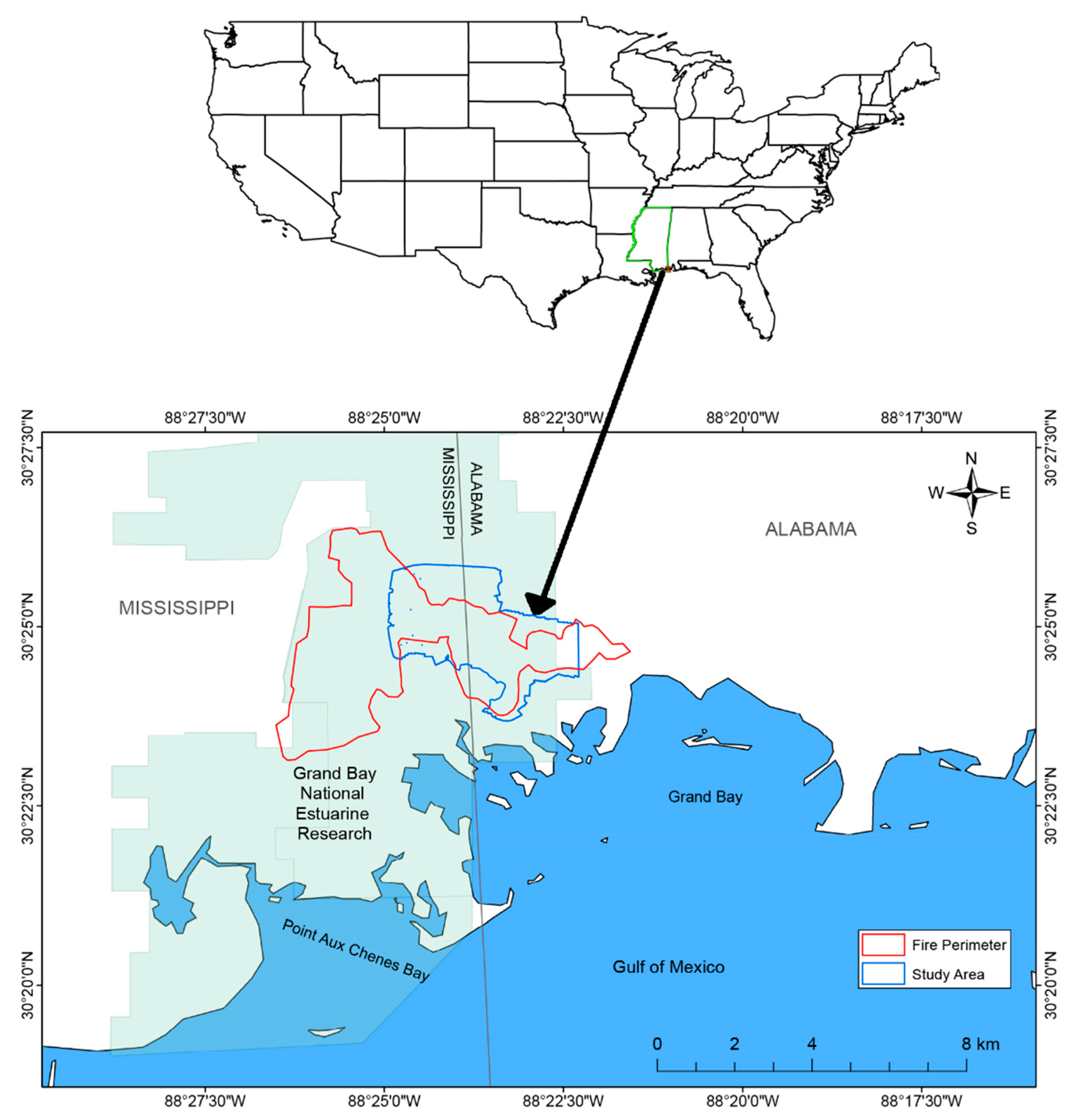
Located in southeast Mississippi and southwest Alabama, the Grand Bay National Estuarine Research Reserve/National Wildlife Refuge (GBNERR/NWR) is a 7400 ha site that is one of the 29 coastal sites designated to protect and study estuarine systems in the USA (
Figure 1). GBNERR/NWR includes a variety of estuarine and upland habitats that form a mostly intact coastal watershed (
Figure 1). Primary estuarine habitats include open water, submerged aquatic vegetation, vegetated salt marshes, and non-vegetated salt flats. Upland areas include wet pine savannah, coastal bay head and cypress swamps, freshwater marshes, and maritime forests. Many of these habitats depend on the regular occurrence of fire, which is critical for maintaining a highly diverse community of plants and animals. However, in the past few decades, fire suppression has led to habitat degradation and the accumulation of woody fuels, predisposing some areas to wildfire [
29]. The details of the species located in GBNERR/NWR can be found in [
30].
The Grand Batures wildfire burned 1719 ha of estuarine and upland habitat within the GBNERR/NWR in February 2016. The UAS data used to map the burned area were collected on February 25 2016 (
Figure 2). To study post-fire regeneration, a small portion of the burned site (approximately 66 ha) was chosen to analyse UAS data. To study the pre-fire (October 2014) health and post-fire (June 2016) regeneration for the entire region, a National Agricultural Imagery Program (NAIP) dataset collected via human-crewed aircraft was used [
31,
32].
2.2. Sensor Descriptions
The multispectral sensor used in this study is a MicaSense RedEdge (MSRE), a sensor specifically designed for small UAS and precision agriculture. It captures five discrete spectral band snapshots simultaneously with a global shutter. Each individual band image was 1280 × 960 pixels with a radiometric resolution of 12 bits. The five bands are blue (centered at 480 nm with a bandwidth of 20 nm), green (560 nm, 20 nm), and red (670 nm, 10 nm), red-edge (720 nm, 10 nm) and NIR (840 nm, 40 nm).
The NAIP four-band multispectral imagery used to assess pre- and post-fire was collected by USDA using Leica ADS100. This push broom sensor captures a total of 13 lines with 20,000 pixels each. The four bands are blue (centered at 465 nm with a bandwidth of 60 nm), green (555 nm, 60 nm), red (635 nm, 32 nm), and NIR (845 nm, 37 nm).
The LiDAR data used for assessing the quality of DSM produced from the UAS imagery were acquired by using an airborne Leica ALS70 multiple pulses in air system. The data were collected at a pulse rate of 273 kHz and a scan rate of 53Hz. The ALS70 sensor can receive seven returns per pulse at 8-bit intensity. The timeline of events and metadata is shown in
Table 1.
BARC is produced from Landsat 7 and/or Landsat 8 multispectral data. NIR (band 4, centered at 830 nm with a bandwidth of 140 nm) and short-wave infrared (SWIR) (band 7, 2220 nm, 260 nm) bands were used to compute the fire severity product.
2.3. UAS Imagery-Derived DSM and Orthomosaic Production
The cloud-based MicaSense Atlas platform was used to produce an orthomosaic and a DSM from the UAS-collected imagery. White reference panels were used during the UAS flight to allow Atlas to perform radiometric corrections of the orthomosaic. In total, UAS flights produced 4535 images for each MSRE band. At 305 m above ground level (AGL), the ground sampling distance was 0.2 m/pixel. The UAS imagery collected had 60% side overlap and 70% in-track overlap for creating the orthomosaic and photogrammetry-derived DSM.
The Atlas software generated an orthomosaic by identifying tie points in overlapping images and using those to obtain the correct camera orientation at the time of each image capture. The combination of tie points and camera orientation were used to produce a point cloud, where each point had associated X (longitude), Y (latitude), and Z (height) components. The MSRE imagery had sufficient overlap such that errors were minimized in the placement of tie points between individual images in the mosaic. Mosaic edges were cropped so that images with little overlap did not affect final data analysis.
Atlas produced a DSM from the point cloud, which gave a three-dimensional (3-D) view (top-level surface features) of the target site. Projecting aligned images onto the DSM produced an orthomosaic that covered the entire flight area from a nadir perspective. Since no ground control points were used in data collection, the Atlas-produced mosaic does not align with the NAIP or BARC datasets. To improve the georeferencing accuracy, post-correction of the UAS-derived DSM and mosaic was performed using ESRI ArcGIS [
33].
2.4. Validation of UAS-Derived DSM
The UAS-derived DSM was used to calculate the area and volume of the burned vegetation. To check the accuracy of the UAS-derived DSM, the DSM elevation data were compared with first-return LiDAR elevation data [
34,
35]. A Leica ALS70 500 kHz multiple pulses in-air sensor was used to collect LiDAR data from a human-crewed aircraft. The Leica sensor collected up to four returns per pulse as well as intensity data. The airborne LiDAR data were collected and processed to meet a maximum nominal post spacing of 0.7 m. LiDAR data collection flights occurred March 6 2015 at an altitude of 1981 m AGL with an average ground speed of approximately 280 km/hr. The mean vertical error of the LiDAR dataset was 0.061 m with a standard deviation of 0.060 m. Geographic features that would not have changed (e.g., roads, buildings, individual trees) between data collection periods were used as points (44 points used) for comparing the elevation values produced by the DSM and LiDAR datasets (
Figure 3). The validation analysis shows that the UAS-derived DSM can be a good proxy for LiDAR-derived DSM, with the regression coefficient of determination R
2 of 0.97 (
p < 0.0001) and the root mean squared error between the LiDAR observed and UAS-derived DSM elevations being 1.29 m.
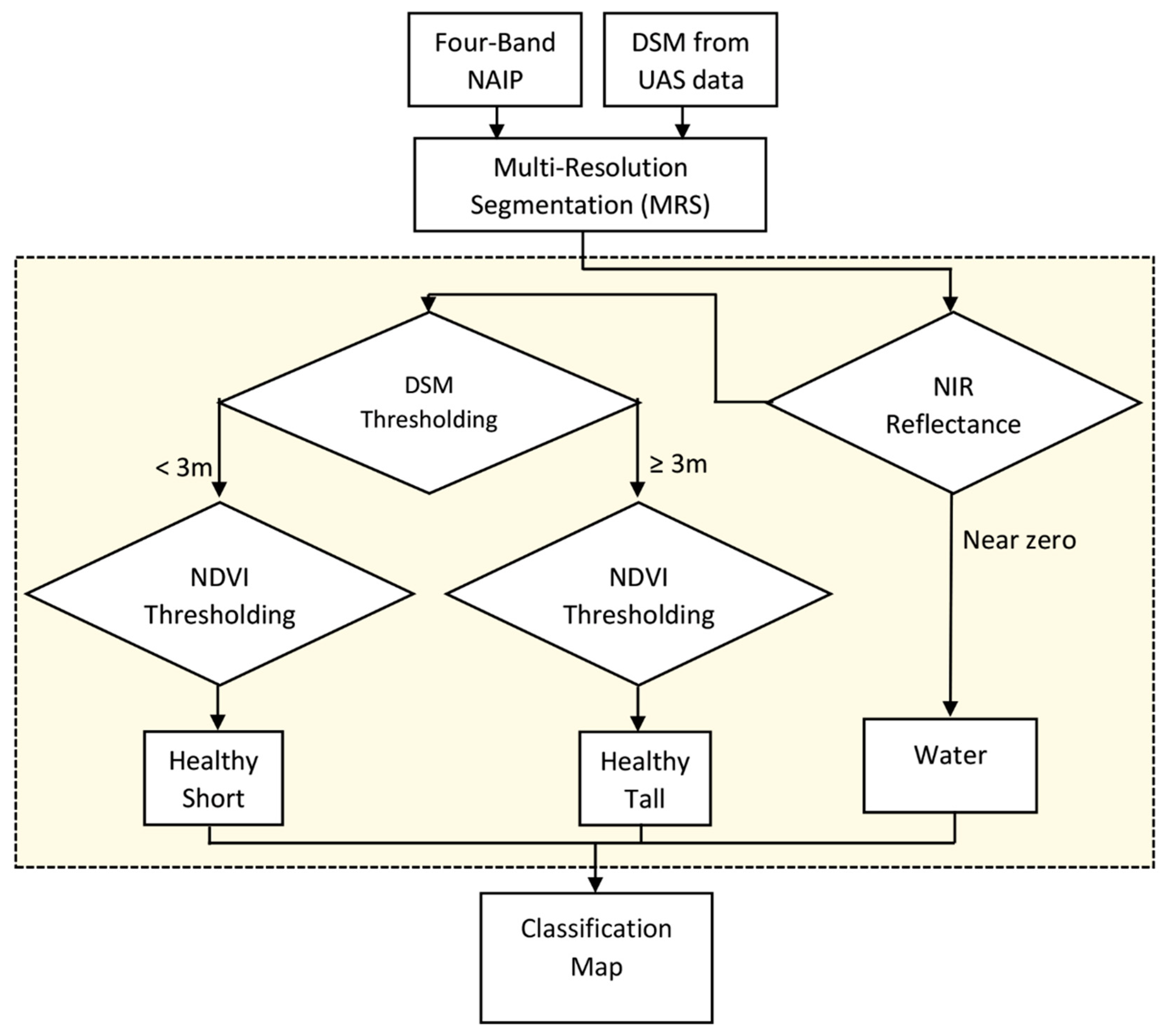
2.5. Hierarchical Classification of UAS and Human-Crewed Aircraft Imagery to Assess Burned Vegetation
The classification methodology (
Figure 4 and
Figure 5) used an OBIA approach on pre-fire (NAIP 2014), immediate post-fire (UAS), and post-fire data (NAIP 2016). Both NAIP datasets were orthorectified in a tiled format, with the caveat that each tile may contain up to 10% cloud cover. The 2014 NAIP dataset has a 1 m ground sample distance (GSD), and a horizontal accuracy of ±6 m at a 95% confidence level, whereas the 2016 NAIP dataset has a 0.6 m GSD, with a horizontal accuracy of ±4 m at 95% confidence level. To improve the georeferencing accuracy, the post-correction of the NAIP imagery was performed using ESRI ArcGIS [
33].
The classification method implemented in this work depended on the following properties:
(1) NIR is primarily reflected by healthy green vegetation, which results in high reflectance values of the NIR band (which produces high values in the normalized difference vegetation index (NDVI)) in regions of healthy vegetation and low values in regions of little or no vegetation (i.e., water and wet soil) [
36];
(2) The DSM layer provided the height information of each pixel in the imagery, which can be used to delineate tall and short vegetation from one another.
The OBIA classification extracts objects from the imagery through image segmentation. Objects are image features such as trees, roads, buildings, lakes, rivers, or any meaningful structure with similar spectral and spatial properties that humans can interpret from remotely sensed data. The multi-resolution segmentation (MRS) algorithm from Trimble’s eCognition OBIA software was used to extract image objects for classification [
37]. The MRS creates image objects using an iterative algorithm, where individual pixels in the image are grouped into an object based on the homogeneity criteria, which are composed of scale, shape-colour ratio, and compactness, that define the total relative homogeneity [
38].
The scale parameter controlled the size of the image objects produced by allowing more spectral variation for larger objects and less spectral variation for smaller objects. Higher values of scale parameters result in larger image objects and reduced processing time. Lower scale parameter values produced smaller image segments at the expense of longer processing time for both segmentation and classification. For the NAIP and UAS classifications, a scale parameter value of 60 was used, which produced smaller objects considering the high-resolution nature of the imagery.
The shape-colour ratio defined the weighting between the image object shape and its spectral colour. A zero weight considered only the colour of the object and a non-zero weight considered the objects shape along with colour, thereby producing smoother object boundaries (reduced fractal boundaries). The compactness parameter described the complexity of the image object boundaries when compared to a circle. For the NAIP and UAS classifications, an empirically-derived shape-colour ratio of 0.1 and compactness of 0.5 were used.
The image objects produced by MRS were then subjected to hierarchical thresholding. The elevation values from the UAS-derived DSM and NDVI were used as features. These features were computed for each object produced by MRS. The histogram of DSM and NDVI values provided threshold estimates. For the healthy tall class, the NDVI thresholds were from 0.49 to 1.0. The other classes are healthy short (0.5–1.0), burned tall (0.2–0.49), and burned short (0.38–0.5). The outputs of thresholding resulted in a set of objects with assigned class labels. Objects with similar labels were combined to form final classification maps.
To assess the regeneration of vegetation in the study area, NAIP multispectral data were utilized along with the UAS-collected imagery. For pre-and post-fire NAIP data, the classes considered were water, healthy tall, and healthy short vegetation. The classification process considered vegetation taller than 3 m as tall (trees) and vegetation shorter than 3 m as short (marshes). The classes considered for the UAS image classification were healthy tall and short vegetation, burned tall and short vegetation, and water.
Classified regions were exported from eCognition as georeferenced rasters with the same resolution as the original UAS or NAIP data. Classified regions were also exported as shapefiles in order to calculate the area and volume of different classes in ESRI ArcGIS. The areas of healthy vegetation classes were computed using the ‘Zonal Statistics’ tool in ArcGIS. The volume computed was the product of the previously calculated area and the UAS-derived DSM. Since corresponding elevation values were not available for the NAIP imagery, UAS-derived DSM values were used as a proxy.
2.6. Comparison of UAS and Satellite Image Classifications
To demonstrate statistically meaningful accuracies, assessment components (i.e., area frame), as described in remote sensing literature, were used [
39,
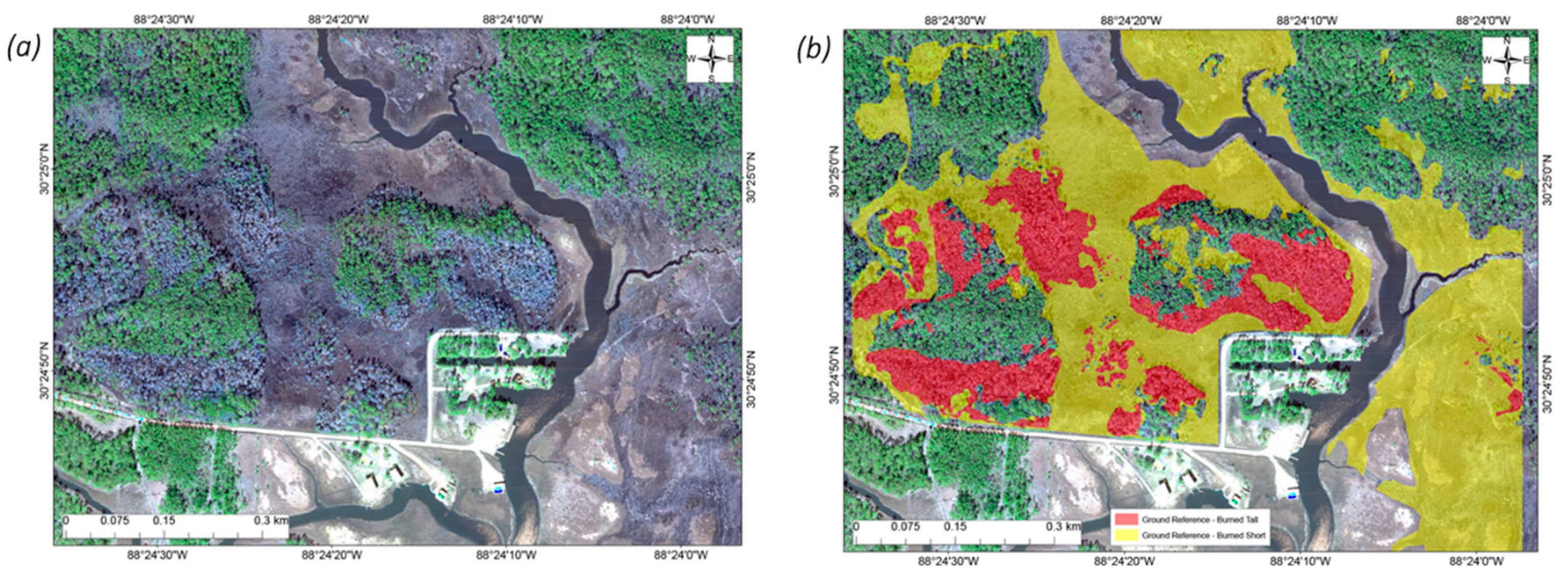
40]. The area frame consisted of a georeferenced orthomosaic that encompassed the region affected by the wildfire. The areal sampling unit used in this study is a 0.2 m pixel. A systematic sampling design with a regular grid, which was determined by the resolution of the orthomosaic product (approximately 0.2 m), was utilized. For response design, an approximately 66 ha spatial support region that consisted of appropriate land cover classes (burned tall and burned short) was chosen (
Figure 6). The ground reference (GR) classification consisted of a combination of field visits and an expert marking the boundaries of the burned areas by visual inspection of the high-resolution UAS orthomosaic. This process involved walking along the patch boundary, determining polygon vertices using a handheld GPS unit (Trimble Geo7X) with sub-decimeter accuracy, and digitizing boundaries from visual inspection of the UAS-obtained imagery. The labelling protocol involved assigning a single class to each polygon areal unit as a short or tall burned vegetation type. The accuracy assessment (
Table 2) only covers the chosen spatial support region. For comparison, the same spatial support region was used to assess the accuracy of the BARC product. BARC is a satellite-derived post-fire vegetation classification map (27 m GSD) generated from NIR and mid-IR reflectance values. BARC is produced by the United States Geological Survey (USGS) and the United States Department of Agriculture (USDA) Forest Service Remote Sensing Application Centre for wildfire incident response [
27].
The performance of the UAS hierarchical classification framework and BARC map were compared with respect to the following accuracy measures: (1) Kappa accuracy (κ), (2) kappa variance (VK), (3) overall accuracy (OA), (4) class accuracies (CA), and (5) 95% confidence intervals (CI). The κ statistic is commonly used in remote sensing literature for studies that measure agreement between classifiers. The κ statistic ranges from zero (representing random chance) to one (perfect agreement between classifiers). OA is the proportion of the classified samples that agree with the reference, which is the GR classification. Comparing the classifiers with the five measures provides a good understanding of the efficacy of different features used in the classification.
3. Results and Discussion
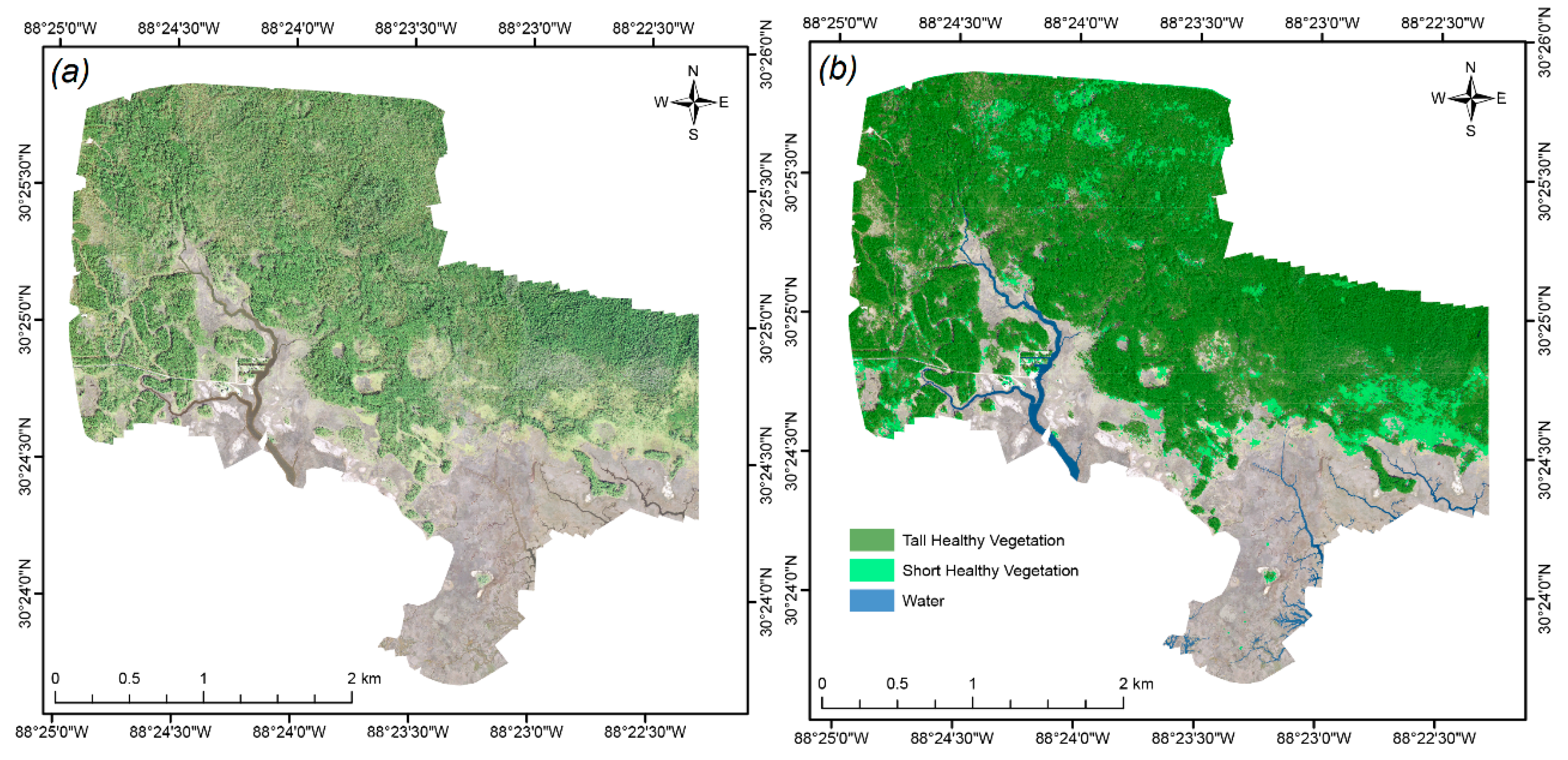
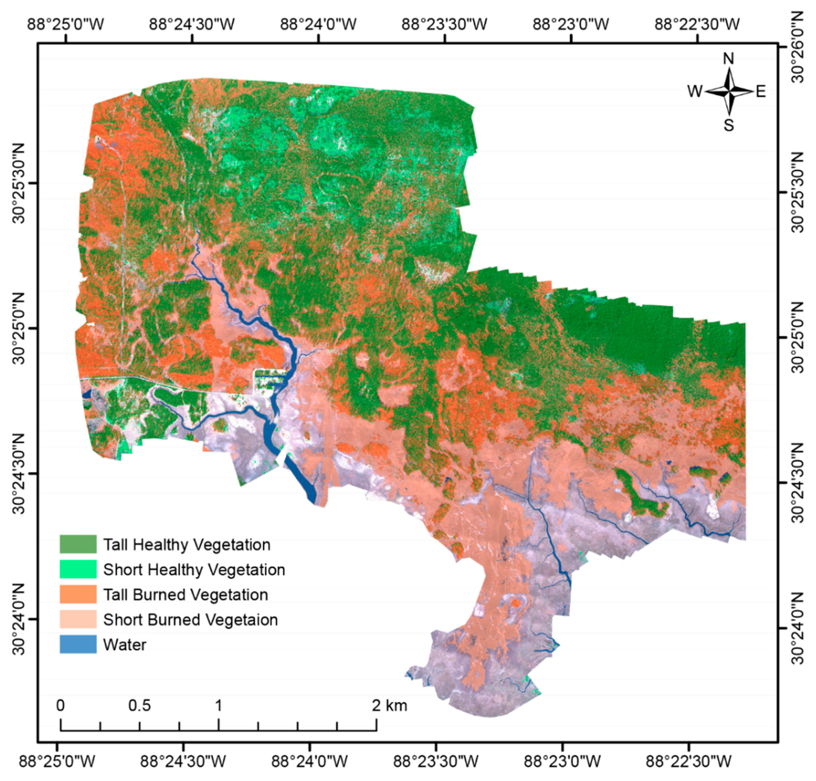
Hierarchical OBIA classification (
Figure 4) was used on the four-band NAIP data to produce a classification map (
Figure 7) estimating vegetation cover 16 months before the wildfire event. Similarly, hierarchical OBIA classification of UAS data (
Figure 5) was used to produce a classification map (
Figure 8) of the site immediately after the wildfire. Individual CAs, OA, κ, VK, and CIs were generated for both UAS and BARC studies (
Table 2). The classification based on UAS imagery had an OA of 78.6% with κ of 0.67 when compared to the GR data (
Figure 6). In comparison, evaluation of the same region via BARC map had an OA of 57% with κ of 0.19, which translates to a slight agreement [
41,
42,
43]. The low κ value of BARC resulted from low CAs for the burned tall and burned short classes.
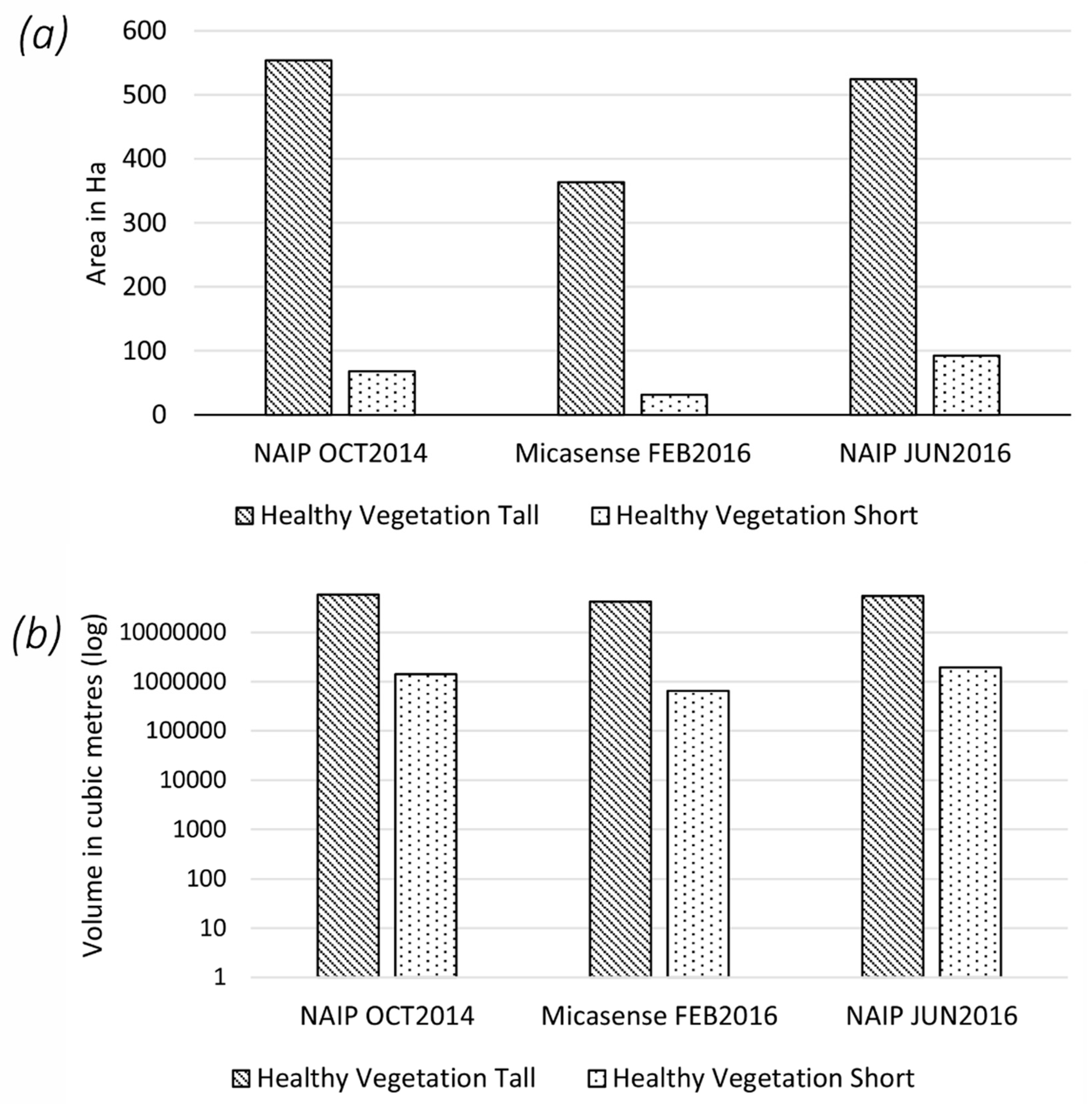
Analysis of vegetation change from pre-fire (
Figure 7), immediate post-fire (
Figure 8), and four months post-fire (
Figure 9) revealed vegetation recovery after the wildfire event. Short vegetation had recovered by four months post-fire (
Figure 9) as the area and volume had higher estimates than the pre-burn levels (
Figure 10). The volume of tall healthy vegetation changed little during the study. However, the area covered by tall vegetation increased from immediate post-fire to four months post-fire (
Figure 10).
The BARC map that was used for comparison with the classification map produced from the UAS data initially had four-classes (high, moderate, and low burn severity classes, as well as an unburned class). The BARC high, moderate, and low burn classes were merged into a single burned class (
Figure 11) for comparison with the UAS classification map.
The BARC map underestimated the burned extent compared to the map produced from the UAS-collected imagery using the OBIA classification (
Figure 12). The BARC map failed to delineate most burned areas in regions dominated by short (<3 m) graminoid (i.e., grass-like) plant species, which was likely due to the low resolution of the satellite data as the pixels were mixed (spatially) with the background (possibly soil and marsh). However, the classification map obtained from low-altitude, high-resolution UAS imagery produced a highly accurate delineation of such stands (
Figure 12b, label P1) that were correctly detected as burned areas. Similarly, the BARC map misclassified regions with large unburned trees as burned when they were not considered burned by the UAS classification.
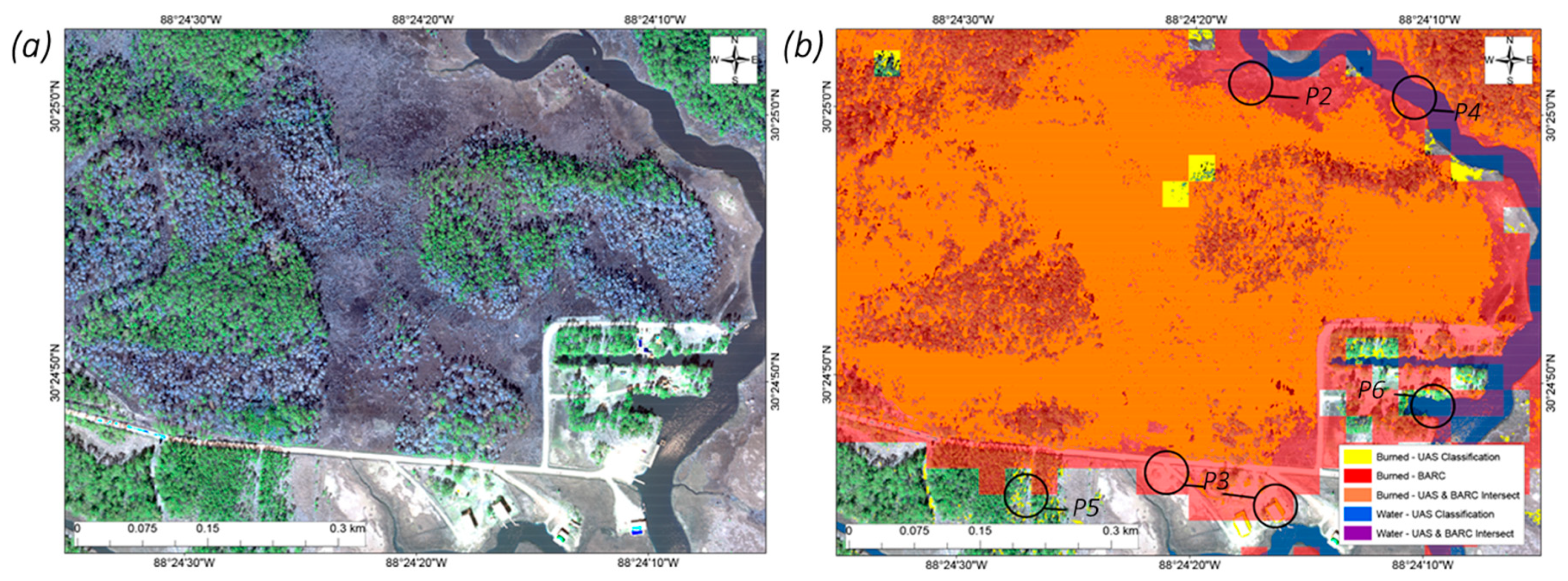
Alternately, other regions of the BARC map show a greater extent of the burned area than the UAS classification map (
Figure 13) due to spectral similarities of some unburned regions with that of burned areas. False positives can be due to low-lying marshes (
Figure 13b, label P2), human-made objects (
Figure 13b, label P3), and water (
Figure 13b, label P4) that may show responses in the NIR and SWIR bands that may appear similar to some burned areas. Ground observation verified these areas (
Figure 13b, labels P2–P4) to be unburned regions.
To minimize shadows in the imagery, UAS imagery was acquired during an optimal time window around solar noon (10:00 to 15:00). However, small regions of shadows were still present, which the UAS-based classification misidentified as burned areas (
Figure 13b, label P5). These shadow regions contributed a tiny percentage of total pixels in the imagery and were unlikely to noticeably influence classification accuracies.
The OA of the UAS classification map was improved by considering water as a separate class. The BARC map considered water as burned in some regions (
Figure 13b, label P6). A mixed pixel similar to that of a burned region can be produced in the BARC map due to water absorption of most or all NIR light, near-water vegetation spectral responses, and the coarse GSD of the satellite imagery. Given the above caveats, the UAS classification map produced a more accurate burned area estimation in these regions than the BARC map.
Some limitations existed in choosing the LiDAR data as these data were not acquired at the same time as the UAS data. Thus, comparing the two datasets was challenging as the landscape had changed during the interim. Additionally, the UAS-derived DSM had a more non-porous and uniform surface on forested areas as the UAS imagery did not penetrate the foliage. In contrast, LiDAR has some foliage-penetrating ability and an increased chance of traveling through foliage gaps, which results in a more porous and non-uniform surface in forested areas. While first returns were used for this study, these factors may still lead to misalignment between DSMs derived from each source.
The UAS-derived DSM had some irregularities in areas where the imagery was saturated, which can occur when a sensor receives too much light (i.e., specular reflection), which may drive pixel values to the maximum allowed by the imaging sensor. Additionally, homogeneous regions/objects on the image surface can generate false elevation values due to lack of tie-points in the imagery, which can affect the accuracy of the UAS-derived DSM.
At similar times of the year, little deviation existed between UAS and LiDAR elevation values (R
2 = 0.97,
Figure 3). While 60% side overlap and 70% in-track overlap may not be sufficient for rigorous volumetric assessments, it was suitable for our analysis of this region (
Figure 3).
Area and volume estimates of healthy vegetation in the burned regions were made from UAS-collected data (
Figure 10). Higher classification accuracies from UAS-collected imagery should produce more accurate volume and area estimates than those of lower resolution satellite imagery. Classification maps produced from UAS and NAIP imagery were used to compare the area and volume of vegetation from pre-fire to both post-fire dates. Volume and area of healthy vegetation had recovered or exceeded pre-fire levels by the second post-fire date (
Figure 10). However, volume estimates for both NAIP datasets were based on the UAS-derived DSM as NAIP DSMs were not available. Thus, there is likely some error in the volume estimates of vegetation from the NAIP datasets. Future data collection events with a UAS mounted sensor would allow for better post-fire vegetation volume estimates as there would be a post-fire DSM to use for volumetric calculations.
The UAS-derived classification map had higher accuracy than the BARC product with respect to the GR (
Table 2). This increase in accuracy is mostly attributable to the increased spatial resolution of the UAS imagery [
22]. Due to the GR regions location inland, the BARC map accuracy assessment tends to show greater misclassifications near areas of low elevation close to the water that are predominantly vegetated by graminoid species (
Figure 11,
Figure 12 and
Figure 13). The reasons for BARC misclassifications include pixel mixing of Landsat imagery, wet soil, and sediment in the water. The SWIR used in the BARC responds with smaller values for healthy vegetation and water and higher values for soil. The NIR band yields higher values for healthy vegetation and lower for burned and unhealthy vegetation. With small graminoid species with a soil background, larger pixels tend to get mixed with a small percentage of vegetation and a higher percentage of soil. Due to coastal vegetation tending to produce lower NIR responses, the combination of the SWIR and NIR response may lead to the classification of pixels as burned when they are not. In addition, areas near water or over water may produce low SWIR values but will also lack much vegetation to give a high NIR response, leading to a burned pixel classification as well. Significant water sedimentation may also produce a higher SWIR response, producing a classification that will appear as a low severity burn. Extending the GR region to graminoid-dominated low elevation regions should show higher UAS classification accuracies and lower BARC accuracies of the entire burned region. This would also provide an even more accurate comparison between the UAS-obtained classification map and the BARC map.
In comparison with previous studies, our approach differs in five key ways: (1) The use of UAS-derived DSM as a feature for classification in addition to NDVI; (2) the use of image objects rather than pixels to produce pre-and post-fire classifications; (3) the use of a relatively inexpensive small UAS and a commercially available sensor in place of satellite, human-crewed, and medium to large UAS fitted with more expensive sensors [
44]; (4) The high spatial resolution multispectral imagery used in this approach, shown to be useful in heterogeneous burned areas in comparison with coarse resolution higher altitude platforms [
22]; (5) our approach directly compared the satellite-based classification product with the UAS classification in terms of kappa statistic, class accuracies, and overall accuracy. The NDVI is oriented towards measuring vegetation health, whereas the normalized burn ratio (NBR) is more suitable for burn severity. Our approach uses a low-cost multispectral sensor that is not capable of sensing SWIR. Instead, NDVI and DSMs were used to classify burn areas as opposed to burn severity, which is what was measured by NBR. NDVI may not be as effective in producing a burn severity map, but our work shows that it can be used to effectively study the vegetation regeneration and fire extent after a wildfire event as effectively as NBR. Satellite-based imagery with SWIR may work better for classifying denser canopies, since it uses NIR and SWIR bands, whereas our approach uses red and NIR bands that are shown to perform moderately well in denser canopies and very well over low-lying sparser graminoid species (
Figure 12 and
Figure 13). Traditionally, pixel-based approaches are used for burn classification and to study vegetation regeneration where salt-and-pepper noise in the classification is prevalent. This warrants a filter-based post-processing technique to improve the homogeneity of pixels [
45]. The OBIA uses both spatial and spectral homogeneity of the pixels to produce a smoother, more understandable, and less noisy classification product.
It should be noted that this study uses imagery collected on three different dates with two different sensors. The spectral response of vegetated areas, consequently NDVI can be influenced by solar angle, shadow, soil moisture, soil color, variations of the atmosphere, and wavelength characteristics of two different sensors [
46,
47]. For the best comparison of spectral values, Jackson et al. suggest that the effect of different response functions on NDVI values may need to be assessed [
47,
48]. Studies done in the past for comparing NDVI values derived from different satellite sensors demonstrated a high correlation with a small shift between values [
49,
50]. Considering that UAS and airborne data used in this work were collected at a much lower altitude compared to Landsat, we did not consider assessing response functions. Readers should consider this while interpreting the results presented in this study.

 ,
, 


