Article

Comparing sUAS Photogrammetrically-Derived Point Clouds with GNSS Measurements and Terrestrial Laser Scanning for Topographic Mapping

1
Civil Engineering Department, Cal Poly University, 3801 West Temple Avenue, Pomona, CA 91768, USA
2
Oak Ridge Institute for Science and Education, Belcamp, MD 21017, USA
3
WestLAND Group, Inc., Ontario, CA 91764, USA
*
Author to whom correspondence should be addressed.
Submission received: 5 June 2019 / Revised: 7 August 2019 / Accepted: 8 August 2019 / Published: 16 August 2019

Abstract

:
Interest in small unmanned aircraft systems (sUAS) for topographic mapping has significantly grown in recent years, driven in part by technological advancements that have made it possible to survey small- to medium-sized areas quickly and at low cost using sUAS aerial photography and digital photogrammetry. Although this approach can produce dense point clouds of topographic measurements, they have not been tested extensively to provide insights on accuracy levels for topographic mapping. This case study examines the accuracy of a sUAS-derived point cloud of a parking lot located at the Citizens Bank Arena (CBA) in Ontario, California, by comparing it to ground control points (GCPs) measured using global navigation satellite system (GNSS) data corrected with real-time kinematic (RTK) and to data from a terrestrial laser scanning (TLS) survey. We intentionally chose a flat surface due to the prevalence of flat scenes in sUAS mapping and the challenges they pose for accurately deriving vertical measurements. When the GNSS-RTK survey was compared to the sUAS point cloud, the residuals were found to be on average 18 mm and −20 mm for the horizontal and vertical components. Furthermore, when the sUAS point cloud was compared to the TLS point cloud, the average difference observed in the vertical component was 2 mm with a standard deviation of 31 mm. These results indicate that sUAS imagery can produce point clouds comparable to traditional topographic mapping methods and support other studies showing that sUAS photogrammetry provides a cost-effective, safe, efficient, and accurate solution for topographic mapping.

1. Introduction

Topographic maps are critical geospatial data products used in earth surface studies that provide insights on environmental conditions, geomorphology, and other earth surface processes and features. Typical methods for topographic mapping, particularly small to medium spatial extents, consist of total station (TS), global navigation satellite system (GNSS), terrestrial laser scanning (TLS), or airborne light detection and ranging (LiDAR). Mapping professionals most often rely on TS and GNSS for producing as-built plans, site-monitoring, and general topographic surveys due to their high levels of accuracy; however, they are time-consuming and costly, especially for medium-to-large-sized topographic mapping projects (≥0.15 km).
TLS has recently experienced a growing adoption rate due to falling costs and smaller form factor designs, turning it into an industry standard for mapping professionals, specifically when fine details are required to be mapped and modeled. However, it is limited to line-of-sight and it is inefficient in areas with many physical barriers and moving objects. In those cases, airborne LiDAR may be preferred over TLS as it is able to capture complete site information rapidly. Airborne LiDAR can successfully evaluate large areas to perform agricultural, geomorphological, and environmental applications [1] and provide enough detail to detect changes or evaluate physical damage [2]. However, issues arise when airborne LiDAR is not accompanied with high-resolution imagery that is needed to support change detection or provide insights on the existing conditions requiring a visual perspective [3]. Furthermore, it is costly and may not provide sufficient details required for topographic mapping when fine-scaled surface features are needed.
Small unmanned aircraft systems (sUAS) have been increasingly employed to capture images that can generate high-resolution point cloud measurements of the terrain using digital photogrammetry at very low cost, a feature attractive to a mapping professional who cannot afford traditional methods. sUAS were initially known for their role in military applications as “drones,” but the use of sUAS in civilian applications, such as construction, is rapidly growing [4]. sUAS have been deemed useful for tasks varying from post-disaster reconnaissance [5] to construction safety applications [6]. Rather than risking lives and sending surveyors into compromised structures after a disaster, sUAS are able to remotely detect damage at a safe distance [7]. Data from sUAS have also been used with echo soundings to conduct bathymetric surveys [8], fatigue crack detection in the inspection of steel bridges [9], and masonry [10]. The Federal Aviation Administration (FAA) has estimated that as many as 7500 commercial sUASs operated in US airspace in 2018, with a value of 13.6 billion dollars [11].
Cameras on commercial off-the-shelf sUAS platforms can easily provide 3D remote sensing capabilities that eliminate the need for expensive scanners [1]. Studies using sUAS include the collection of construction material information, voltage transmission line inspection, enforcing safe practices on construction sites, homeland security rescue operations, forest fire detection, natural resources, forest monitoring, geology, and delivery of goods [12,13,14,15,16,17,18,19,20,21]. Advancements made in digital photogrammetry software have revolutionized the field of sUAS data collection and analysis, allowing engineers and scientists to generate high-resolution topographic maps with low-cost optical cameras [22]. This software has the ability to produce orthorectified imagery maps (orthophotos), point clouds and digital surface models (DSM) at spatial resolutions in the order of centimeters [1,23]—a quality vital to topographic mapping applications [5,24,25,26,27,28,29,30].
Although there have been several studies that evaluate the accuracy of DSMs derived from sUAS equipped with optical cameras, the causes for highly variable accuracy is not well understood, as described by Smith and Vericat [31]. Several factors that may affect sUAS-derived products, are flight parameters, flight speed, flight direction, orientation of the camera, camera focal length, image quality, processing software, topography of mapping area, and type of sUAS (rotary or fixed wing). The combination of several or a single factor may influence the overall accuracy. For example, Manfreda et al. [32] evaluated different flight combinations and the distribution and number of ground control points (GCPs) to reduce the error of the 3D model for monitoring a dam. However, their study sample is limited to evaluating sixteen checkpoints and not several thousands of points as those found in point clouds, which is necessary to deeply understand the behavior of the derived 3D model. The horizontal and vertical accuracy reached was 0.20 cm and 3.5 cm, respectively, which is higher than what is allowed for many engineering applications, particularly in the vertical component (e.g., civil and surveying engineering). These limitations are similar for several other studies, where they solely compare the accuracy between a limited number of checkpoints and not the overall 3D model within the area mapped [25,26,33,34,35,36,37,38,39,40,41,42,43]. The results achieved in these studies are highly variable requiring the need for thorough evaluations comprised of a greater sample.
Salach et al. [44] evaluated the vertical accuracy of digital terrain models (DTMs) derived using LiDAR and photogrammetry in uncovered and vegetated areas. The results provided an insight on the possibilities of sUAS equipped with an optical camera and LiDAR, however, the number of checkpoints used is limited to thirty five and the accuracy observed for them was low for both the horizontal and vertical component, where the X and Y errors observed were 0.061 m and 0.063 m, and 0.068 m for the Z error. Additionally, the airborne LiDAR data used as ground truth for comparison had a low density of 4 points per square meter and a vertical accuracy of 0.15 m. Naumann et al. [45] performed an accuracy comparison between TLS and sUAS derived DSMs at a dike for coastal engineering, where they were able to observe a STD of 0.040 m between the sUAS and TLS point clouds for over 680,000 points. However, a large number of GCPs (11) were used to maximize the accuracy results, which is more than desired by most practitioners, especially for a study area with simple geometry. Espositoa et al. [46] evaluated the performance between a sUAS derived point cloud and TLS for 3D reconstruction of a building. In their study, they were able to achieve a global accuracy of 0.10 m and better than 0.05 m for local measurements. Although the results seemed promising, the two different point clouds had to be manually aligned followed by automatic alignment and optimized to fit using 20 GCPs, which does not provide an independent evaluation amongst the two different mapping methods. For these reasons, it is critical to test point clouds from sUAS photogrammetry against traditional mapping methods to evaluate their suitability for topographic mapping, especially when accurate point clouds are required in the centimeter-level range.
In this study, we evaluated the accuracy of a point cloud derived from sUAS imagery by comparing it to GNSS real-time kinematic (RTK) and TLS ground truth measurements of a parking lot. GNSS-RTK is a conventional mapping practice that achieves high-accuracy positioning ranging in the ±2 cm level, while TLS is capable of high-accuracy positioning in the ±5 mm level. Both of these mapping techniques offer high-accuracy positioning and are commonly used in topographic mapping. sUAS technology has been shown to compute earthwork quantities with high accuracy, [36,47], and extensive testing has been performed to illustrate the impact of GCPs [24,25,26,33,34,35,36,37,38,39,40,41,42,43], however, the accuracy of the resulting point clouds has yet to be tested extensively, which is one of the main contributions of this study: to evaluate the performance of a sUAS point cloud comprehensively against GNSS-RTK and TLS mapping methods at areas beyond the GCPs, where the accuracy level reflects how well the sUAS point cloud was fitted to a priori GCPs and does not reflect the overall accuracy in areas away from the GCPs. We intentionally surveyed a flat area since flat scenes are commonly encountered in the field, e.g., agriculture, civil engineering, and construction, which pose challenges for accurately determining vertical measurements. Furthermore, our study provides a detailed workflow on data acquisition that may be replicated to support researchers, scientists, or practitioners in achieving high accuracy sUAS derived point clouds. The data acquisition workflow followed in this study may alleviate aforementioned issues associated with the low accuracy of point clouds derived from sUAS imagery. The primary idea of the data acquisition workflow is to minimize all possible sources of error that typically contribute to the generation of the ground truth data used for comparison (e.g., GNSS and TLS measurements) and the sUAS derived point cloud.

2. Materials and Methods
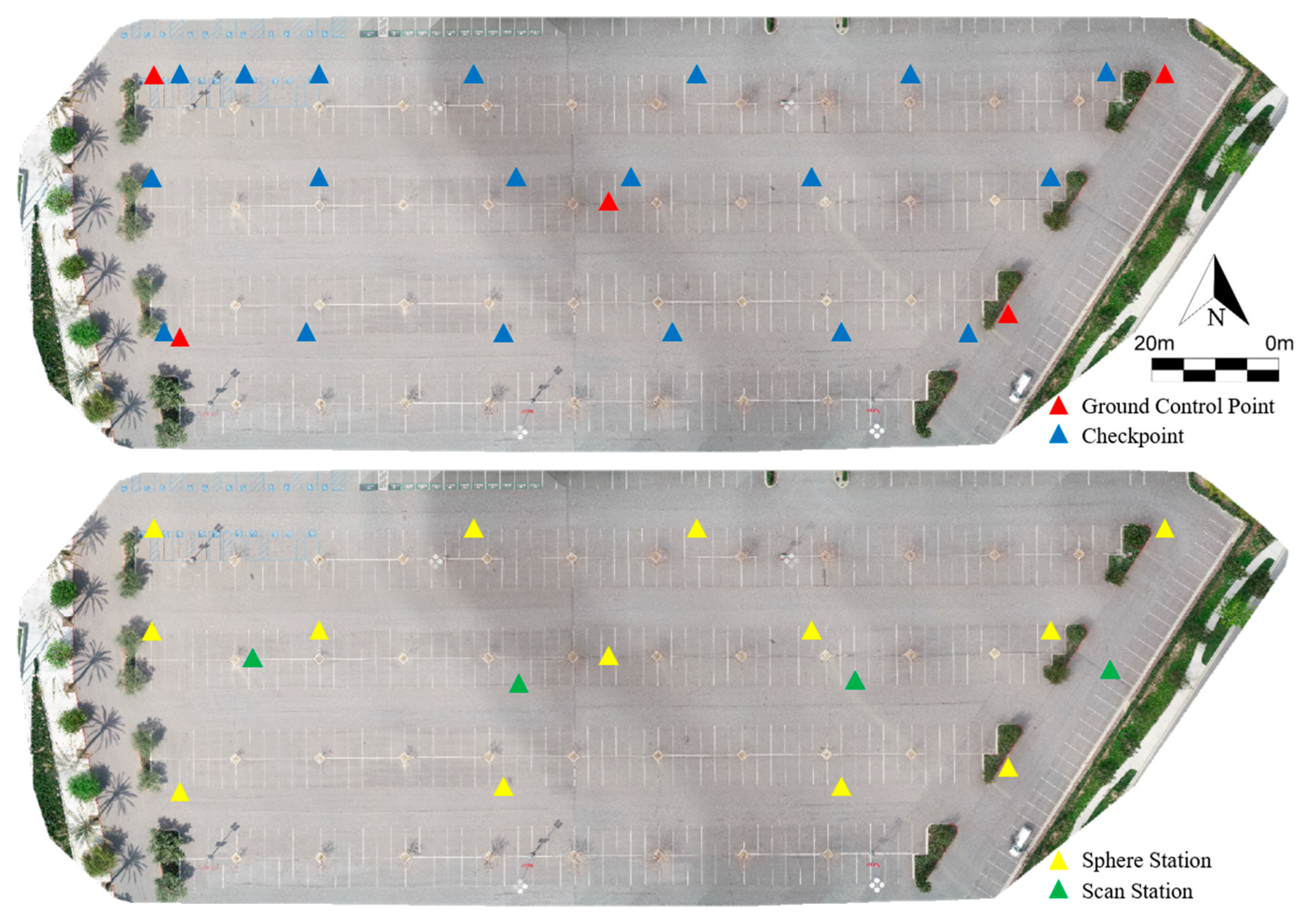
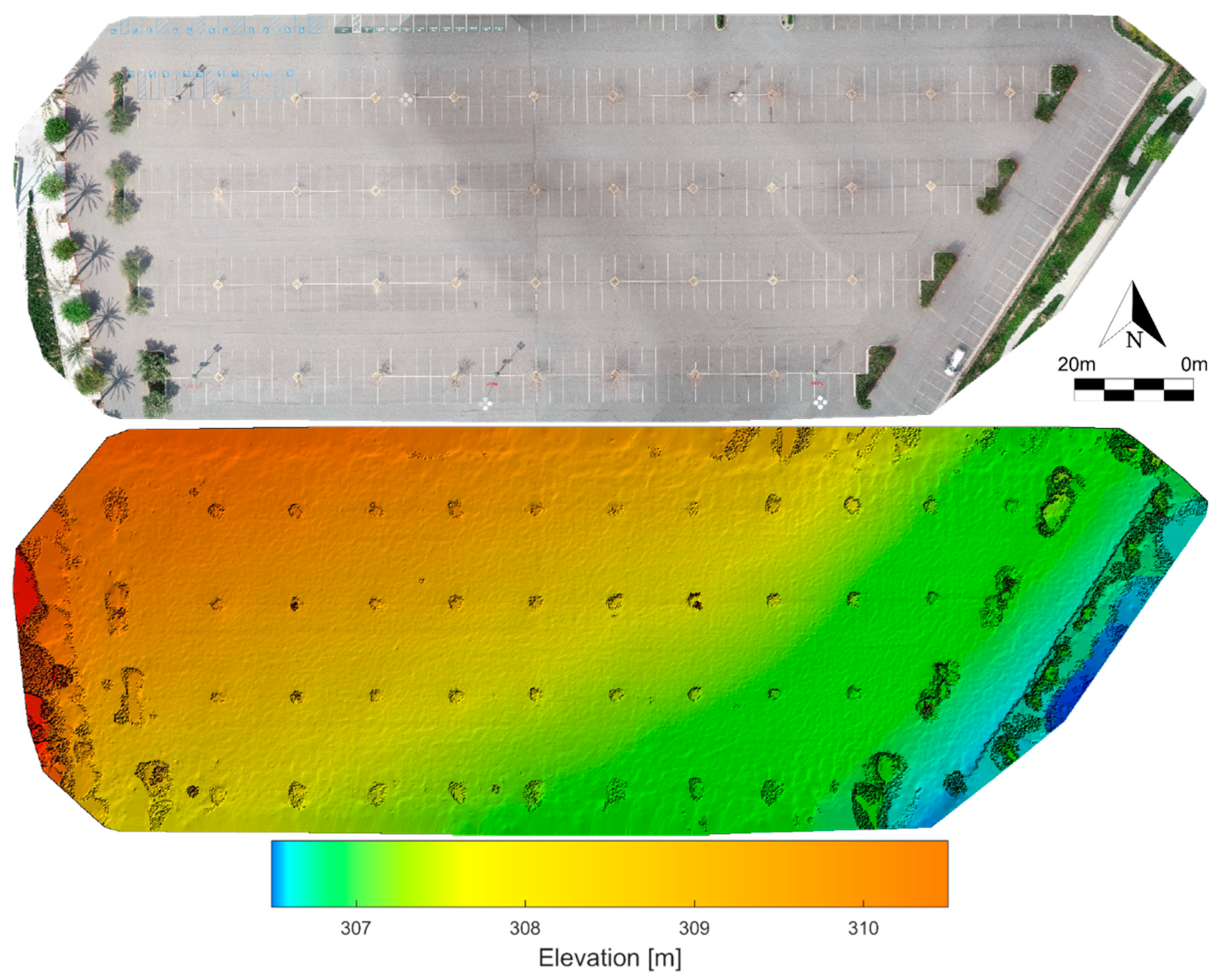
2.1. Study Area

The study area consisted of a relatively flat parking lot at the Citizens Bank Arena (CBA) in Ontario, California (Latitude: 34°04′27.69”N, Longitude: 117°33′40.38”W), having a maximum elevation difference between the lower, east end of the site and the upper, west end of the site of about 4 m. The north-south inclination is much smaller for most areas. The total area mapped was approximately 0.017 km2. Most of the site was paved, except for a few parking lot islands that had trees without leaves. There were several light fixtures distributed throughout as well. We selected this site for its relative absence of vegetation, which can complicate surface modeling and accuracy analysis. Its simple planar geometry and temporal stability make it ideal for comparing the results of different mapping methods over time. The total field time to complete all measurements was 2 hours from arrival to departure, including the sUAS setup, sUAS survey, TLS survey, and GNSS-RTK survey of GCPs and checkpoints. All measurements were connected to the same five GCPs shown in Figure 1. The checkpoints allowed evaluation of the test data for locations outside of the GCPs (see Figure 1), which would have minimum errors since they served as anchor points for adjusting the sUAS point cloud. Figure 1 shows the study area, including the distribution of the GCPs, checkpoints, scan and sphere stations.

2.2. sUAS Image Acquisition

The aerial survey was performed on 5 April 2018, using a DJI Phantom 4 Pro v2.0 sUAS with its factory-installed 20-megapixel camera. The survey area covered approximately 0.017 km2, over which the sUAS flew at about 45 m above the ground collecting images at nadir with a forward overlap of 85% and a sidelap of 75%. The wind speed was 8 mph during the flight, the temperature was 28° Celsius, and the imagery was acquired around midday. The flight lasted 5 min and 46 s and captured 201 images. The flight was performed using the DJI GS Pro application, which constructed an autopilot flight path based on input parameters—such as flying height, forward lap, and sidelap—and executed it in the field. All images contained geotags from the sUAS’s onboard GNSS sensor, which helped with initial photogrammetric alignment but lacked the accuracy required for direct geo-referencing. For high accuracy adjustments, we used an indirect geo-referencing technique utilizing GCPs to adjust and anchor the photogrammetrically-derived point cloud.

2.3. GNSS-RTK Survey

A GNSS-RTK survey established the 5 GCPs and 19 checkpoints using a Trimble R10 rover and base station and a Trimble TSC3 data collector. The rover was set to have a position dilution of precision (PDOP) mask of 4.0, an elevation mask of 15°, and the precision horizontal and vertical tolerances were set to 0.009 m and 0.012 m, respectively, while the base was set to have an elevation mask of 15° and a logging interval of 1 s. The base station used for GNSS-RTK survey collected observations for 2 hours and was placed roughly 100 m away from the rover location, where there was an unobstructed line of sight between the rover and base station. This established a base station accuracy level of 2 cm in the vertical and horizontal components. The rover collected data at each GCP and checkpoint for 3 min, producing 180 GNSS observations, while the base station collected data during the entire survey, producing a total of 7200 GNSS observations over two hours.

2.4. sUAS Point Cloud Generation

After the images were retrieved from the sUAS, the commercial modeling software Pix4D was used to create the sUAS based point cloud. The general framework of Pix4D involves automatic aerial triangulation (AAT), bundle block adjustment (BBA), DSM, point cloud and orthophoto generation. The Pix4D workflow begins with the AAT producing tie points from the images based on similar features in overlapping images, using the GCPs as a reference. Then, after the initial AAT is completed, BBA is used to estimate the internal parameters of the camera, which include the focal length, principal point, radial and tangential distortion, and absolute camera position and orientation parameters for each image. Finally, the process ends when the BBA converges on a solution with an assessment of the adjustment error. From the 5 GCPs used in the BBA, a 3D root-mean-square error (RMSE) of 3 mm was observed and a spatial resolution of 7.5 mm was achieved. The final processing steps consist of the preparation of the sUAS point cloud to be imported into Autodesk ReCap Pro to compress the sUAS derived point cloud and subsequently import into Autodesk Civil 3D for comparison against the GNSS-RTK survey data.

2.5. Camera Self-Calibration

The nonmetric camera self-calibration technique was applied to the “uncalibrated” images by manually identifying 5 GCPs on the images and applying them as constraints to refine the camera self-calibration and georeferencing parameters; therefore, georeferencing relied exclusively on GCPs. Ideally, the camera calibration parameters should be estimated in laboratory settings, however, these parameters often change under in-flight conditions [48], therefore, most practitioners prefer to apply the self-calibration method on a flight-to-flight basis [49,50]. Depending on several factors, such as flight configuration (e.g., flying height, overlap, and image orientation), environmental conditions, surface complexity, purpose of sUAS survey, number and distribution of GCPs, quality of GCPs and the flying and shutter speed, the camera self-calibration parameters can vary [51]. Having a low number of GCPs can lead to a poor self-calibration and may lower the accuracy of the sUAS-derived point cloud, DSM, and orthophoto [51]. Therefore, it is critical to test several self-calibration scenarios to optimize the self-calibration parameters for each sUAS survey.
The estimated internal parameters of the camera in Pix4D, were estimated to be 8.653 mm, 6.403 mm, 4.268 mm, 0.008, −0.022, 0.017, 0.000, and 0.000 for the focal length (f), principal point offset in x- and y-direction (cx and cy), radial distortion coefficients (K1, K2, and K3), and tangential distortion coefficients (P1, and P2), respectively. The mean absolute camera position and orientation uncertainties were estimated to be 3 mm, 3 mm, 96 mm, 0.004°, 0.005°, and 0.001° for X, Y, Z, Omega, Phi, and Kappa, respectively. In addition, the standard deviations of the absolute camera position and orientation uncertainties were estimated to be 1 mm, 1 mm, 2 mm, 0.001°, 0.001°, and 0.000° for X, Y, Z, Omega, Phi, and Kappa, respectively.

2.6. TLS Survey

We used a Faro Focus3D X 330 laser scanner to capture the 3D point cloud, which served as the ground truth for comparing the entire sUAS point cloud. This survey was performed by scanning the parking lot at four scan stations and georeferenced using spheres placed at the five GNSS-RTK surveyed GCPs and eight additional checkpoint locations, visible in all scans. The spheres were placed by using a 2 m rod and bipod at each sphere station. Registration of the four TLS point clouds was performed using Faro Scene software. Upon completing the registration, a visual inspection was performed to ensure proper registration. A spatial resolution of 4.1 mm was achieved by the data collection. The final processing steps are similar to those from the sUAS point cloud, which consist of the preparation of the TLS point cloud to be imported into Autodesk ReCap Pro to compress the TLS derived point cloud and subsequently import into CloudCompare, where the TLS point cloud will be evaluated against the sUAS point cloud.

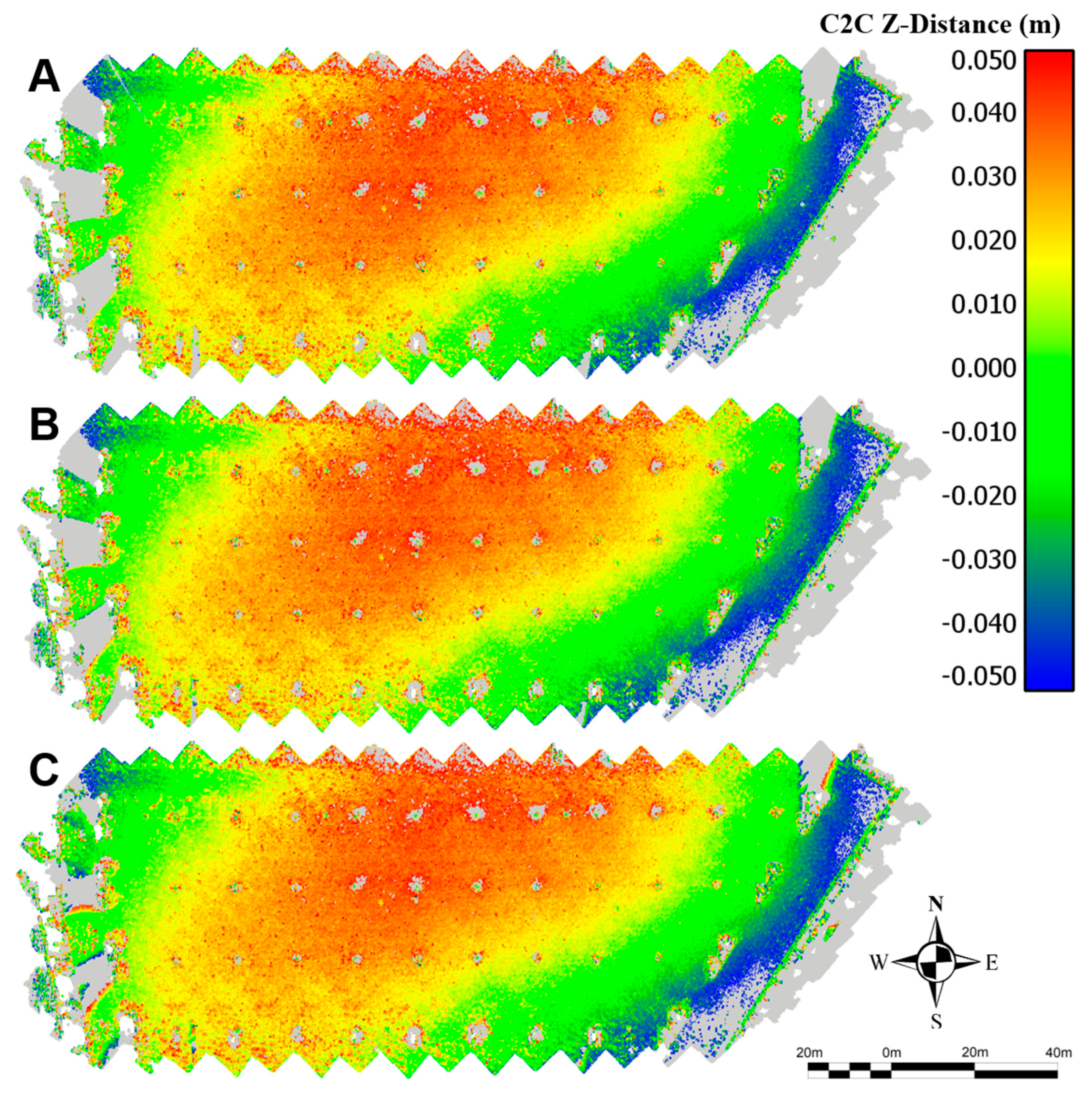
2.7. Point Cloud Comparison (sUAS versus TLS)

The point cloud analysis compared the sUAS and TLS point clouds. It is important to note that performing a cloud-to-cloud (C2C) comparison is challenging due to the irregular point spacing from the sUAS and TLS point cloud datasets, and no commonly recognized method currently exists for assessing point cloud accuracy [52]. The only guide available to evaluate point clouds is given by the Vertical Accuracy Reporting for LiDAR Data by the American Society for Photogrammetry and Remote Sensing (ASPRS) [53]. For these reasons, the vertical component is the most appropriate comparison to perform.
The C2C comparison is performed in CloudCompare by computing the nearest neighbor distance between the reference (i.e., ground truth) and the compared cloud (i.e., sUAS point cloud). In this approach, the Euclidean distance is computed between each point in the compared cloud with the nearest point in the reference cloud. The analysis involved both a tabular summary and visualization to reveal spatial patterns between the two point clouds. The C2C comparison was tested by applying three maximum search distances (0.5 m, 1 m, and no limit) between the TLS and sUAS point clouds to minimize the presence of outliers. These search distances provide an opportunity to perform a thorough evaluation and will help reveal any concerns that need to be addressed that are impacted by the maximum search distance parameter.
The point clouds were evaluated in the raw irregular point spacing form to minimize errors that may be introduced by interpolation techniques that are typically used to grid data to a regular point spacing [54,55]. By comparing the two point clouds without gridding the data and/or introducing interpolation techniques, it provides a true comparison of the point clouds produced from the two mapping techniques. To determine if there are any vertical displacements within the point clouds, it is necessary to provide a quality assessment of the vertical component. To offer a holistic evaluation of the vertical accuracy, we determine the error for the entire parking lot mapped rather than solely evaluating the checkpoints surveyed, as it will reveal spatial trends comprehensively within the test site.

3. Results

The sUAS point cloud yielded a 3D RMSE of 3 mm during BBA at the 5 GCPs, suggesting that the BBA had successfully converged with the GCP anchor points. At face value, this error level appears comparable to, if not better than, most traditional mapping methods (e.g., TLS, GNSS, and TS). However, this accuracy level simply reflects how well the sUAS point cloud was fitted to the a priori GCPs and does not provide a clear indicator of overall accuracy in areas away from the GCPs. Doing so would lead to an ecological fallacy or false inference. This is one of the main contributions of this study: to evaluate the performance of a sUAS point cloud comprehensively against GNSS-RTK and TLS surveying techniques at areas beyond the GCPs. Another contribution of our study is to provide a detailed workflow on data acquisition that may be replicated to support researchers, scientists, or practitioners in achieving high accuracy sUAS derived point clouds. The data acquisition workflow followed in this study may alleviate aforementioned issues with the low accuracy of point clouds derived from sUAS imagery. The primary idea of the data acquisition workflow is to minimize all possible sources of error that typically contribute to the generation of the ground truth data used for comparison (e.g., GNSS and TLS measurements) and the sUAS derived point cloud. The resulting high-resolution orthophoto and DSM from the sUAS survey are shown in Figure 2.

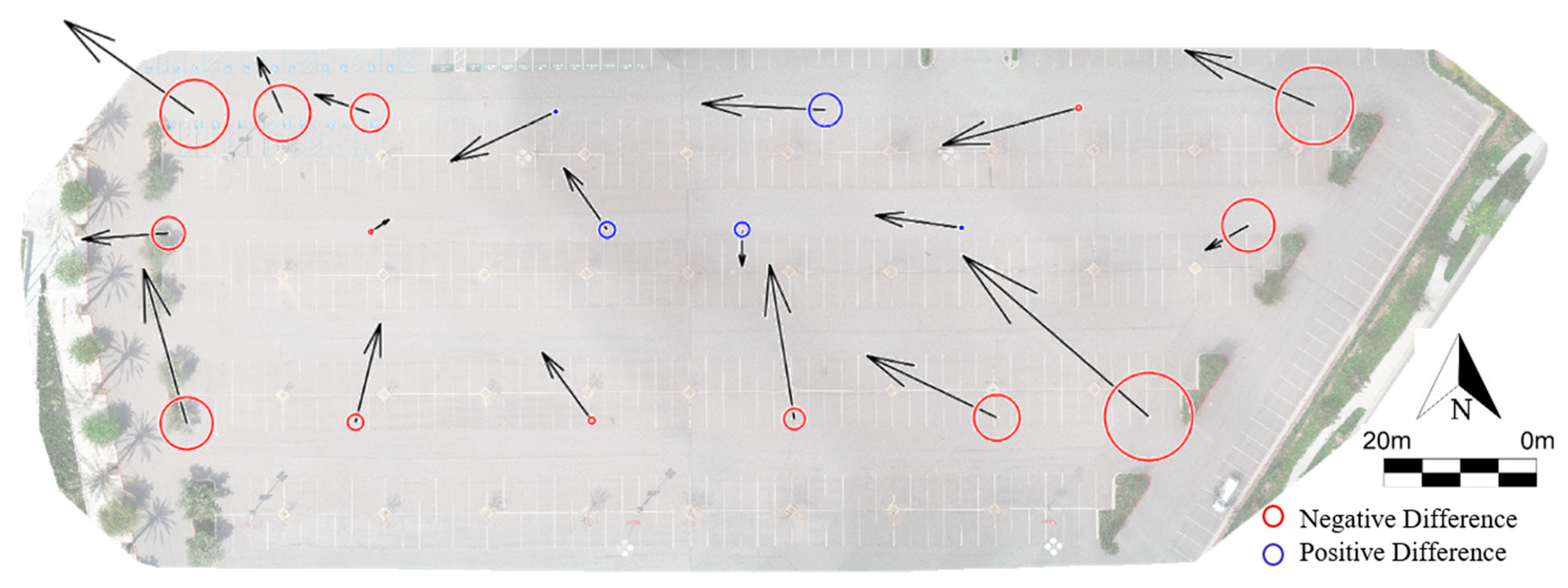
3.1. sUAS versus GNSS-RTK Survey

The GNSS-RTK comparison involved comparing the sUAS point cloud to GNSS-RTK measurements at nineteen checkpoints distributed throughout the test site (see Figure 1), where we evaluated the residuals and statistics in the X, Y, Z, horizontal, and 3D components (see Table 1). A cross-examination of Table 1 highlights the reliability and accuracy of the sUAS point cloud. The table characteristics illustrate minor differences between the two methods, where the RMSE is within the ±2 cm accuracy of the GNSS-RTK measurements for the horizontal component and slightly over ±3 cm for the vertical. The vertical component usually has the largest error for most measurement methods, as in our case (see Table 1). Therefore, the 3D error is generally influenced by the higher values of the vertical.
The spatial plots of the nineteen checkpoint projection residuals are shown in Figure 3. A review of the projection residual plot in Figure 3 highlights the behavior of the sUAS point cloud when the BBA is constrained by the introduction of the well-distributed 5 GCPs. The horizontal residuals are mainly in the north and west directions. In Figure 3, the positive differences signify the positions where the sUAS point cloud is higher than the GNSS-RTK measurements, and the negative differences represent positions where the sUAS point cloud is lower than the GNSS-RTK measurements. It is shown in Figure 3 that the elevations of the sUAS point cloud are primarily lower than those of the GNSS-RTK measurements, which is supported by the characteristics of the statistics shown in Table 1.
By performing this evaluation, we provide an independent assessment of the performance of the BBA since the nineteen checkpoints were not included in the model and were solely compared in Autodesk Civil 3D independently. The five GCPs were evenly distributed on the ground throughout the study area, placed at the corners and at the center. This particular placement of the GCPs for a small rectangular project site of simple geometry provides quality performance for a BBA and minimizes the magnitude of the errors within the point cloud. To emphasize the differences between the sUAS point cloud and GNSS-RTK measurements explored herein, the results obtained highlight the quality of the horizontal and vertical accuracy of the sUAS point cloud. These results are relatively stable and provide confidence that a quality high-resolution point cloud from sUAS imagery is produced when proper procedures are followed.

3.2. sUAS versus TLS Point Cloud

Table 2 shows TLS ground truth registration errors of 3 mm and below for the horizontal and vertical components and under 5 mm overall. This meets the typical industry standard of 6 mm or less for the overall distance error and indicates that a proper registration was performed, making the TLS a reliable baseline for comparing the sUAS point cloud.
Figure 4 illustrates the vertical difference between the sUAS and TLS point clouds. There were a total of 18,933,496 and 69,430,865 points used in the comparison between the sUAS and TLS point clouds, respectively. Overall, the majority of the site exhibits similar spatial patterns amongst the three distinct search distances tested. The sUAS point cloud exhibits higher differences at the center of the test site, likely due to having only 1 GCP at the center, producing a barrel effect in the point cloud comparison. This effect is shown through the edges of the test area exhibiting smaller differences in the range of ±2 cm, while in the midsection it increases to 4 cm.
Table 3 shows the descriptive statistics of the differences between the sUAS and TLS point clouds. It shows average vertical differences of 0.002 m, 0.002 m, and −0.030 m for search distances of 0.50 m, 1-m, and no limit, respectively. The standard deviation of the vertical distance for the search distance of 0.50 m, 1-m, and no limit, are 0.031 m, 0.039 m, and 0.240 m, respectively. Although the overall average differences and standard deviations are relatively small, especially for search distances of 0.50 m and 1-m, they still exhibit a positive bias (i.e., over-estimated) due to noisy outliers in both the TLS and sUAS data, which can be removed manually by filtering the point cloud before performing the C2C comparison. As expected, the unlimited search radius produced the largest average error and standard deviation due to outliers caused by matching unrelated but distant nearest neighbors.
Some of the discrepancies observed may originate from the C2C process where the spatial resolution is lower than desired and the distance amongst the points compared may be larger than preferred. This will provide different elevation values for distinct points within the respective point clouds. Considering the vertical statistical values related to the TLS measurements, the corroboration procedure endorses the high performance of the images acquired by the sUAS. Certainly, the comparison among the sUAS and TLS point clouds could be influenced by artifacts related to the methodology used for point cloud production and the workflow followed to process the sUAS datasets.

4. Discussion

Georeferencing plays a critical role in topographic mapping and other studies of the Earth’s surface. Since the dual-frequency GNSS-RTK measurements served as the baseline for establishing all other coordinates, errors in the GNSS survey would propagate to the TLS and sUAS data. This made it critical to minimize the errors in the GNSS-RTK survey prior to using this data for the TLS and sUAS surveys. To minimize the impact of errors that may be introduced from the GNSS-RTK survey, proper data acquisition and set up procedures were followed, including post-processing of the GNSS-RTK data, a critical step in achieving high-accuracy positioning.
An area of interest in current research involves looking at ways to reduce the errors of surface models through image acquisition techniques and by using different photogrammetric algorithms [32,51]. Technique-based approaches include adjusting flying height, flight pattern, overlap, camera tilt, GCP distribution, and using different photogrammetric software. These studies appear to show that the horizontal accuracy of photogrammetrically derived point clouds is usually better than the vertical accuracy. Therefore, most of the studies primarily focus on the vertical accuracy rather than the horizontal, especially when the point spacing is irregular, for example, point clouds. Prior studies have shown that at minimum four or five GCPs are typically required to produce accurate point clouds [29,56], a primary reason why we chose 5 GCPs. However, the generated point cloud from photogrammetric algorithms is highly impacted by other factors such as flying height, GCP configuration, flight pattern, optical system quality, camera tilt, overlap, and surface complexity. Therefore, the results in this study may be improved in future research, including removing the barrel effect in the point cloud comparison by incorporating additional GCPs in the BBA and testing additional study areas with various terrain characteristics. These additional tests will help verify the results achieved in this study.
The literature [5,24,25,26,27,28,29,30] has shown that sUAS are capable of aiding projects related to the earth’s surface; however, limited studies are available relating to their accuracy in regards to conventional methods, especially GNSS-RTK and TLS surveys. The accuracy results achieved in the study are superior to those found in current literature that aim to assess the accuracy of sUAS for topographic mapping [24,25,26,33,34,35,36,37,38,39,40,41]. This evaluation supported the idea that the use of sUAS can support topographic mapping projects and mitigate the efforts required for accurate point cloud production. The ease-of-use, accessibility, affordability, accuracy, and quality of the high-resolution point clouds derived from sUAS imagery, with the possibility of high temporal frequency, make these systems ideal for monitoring and general topographic mapping.
The accuracy achieved by the sUAS derived point cloud in comparison to the GNSS-RTK and TLS measurements can be linked to the proper preparation, execution, and framework of the aerial survey, GNSS-RTK survey, TLS survey and planning, and to the processing techniques for each mapping method. Proper methods and practices need to be performed with care to ensure that optimal results can be achieved. Otherwise, the quality of the sUAS point cloud may be deteriorated.
Although the results generated were promising, it should be noted that operational challenges will be encountered for employing sUAS photogrammetry due to environmental conditions. For example, weather conditions can affect smooth flight operation and it may cause difficulty in accurate point cloud generation. Therefore, weather conditions should be considered, especially when climate conditions suddenly change. Accessibility to place and locate GCPs and checkpoints along the project site may cause problems. Though sometimes it is considered that all areas within a project site will be accessible, this is not always the case. Some areas are considered inaccessible due to them being unsafe or hazardous, particularly along steep slopes of terrain. Obstructions may also cause challenges and may be found in areas with high relief terrain or in urban environments (e.g., power lines, structures, trees, high vegetation, etc.). These obstructions can deteriorate the quality of the GNSS measurements and limit the line-of-sight between the pilot and sUAS. Nonetheless, as technology continues to advance and sUAS become more affordable, the accuracy of these systems will also improve, and they will become a mainstay technology for topographic mapping.

5. Conclusions

This study assessed the accuracy of point clouds derived by photogrammetry based on sUAS images for topographic mapping. The sUAS photogrammetry method generated a dense point cloud with 7.5 mm spatial resolution using the Pix4D software package to process imagery captured from sUAS and geo-referenced using the GNSS-RTK surveyed GCPs. We found that, when flying at about 45 m, a 3D RMSE of 3 mm at the GCPs can be achieved and residuals of 18 mm and −20 mm for the horizontal and vertical components, respectively, can be attained at the checkpoints. Furthermore, when the sUAS point cloud was compared to the TLS survey, the average difference observed was 2 mm with a standard deviation of 31 mm for the vertical component. These residuals are well within the 2 cm error range of the GNSS-RTK survey, proving that measurements conducted with sUAS with GCPs are comparable to, and in aspects, superior to traditional mapping techniques.
In this study, the distribution and number of GCPs used to generate the dense point cloud were not tested and should be considered in future studies. Assessing the accuracy of these point clouds is a critical step towards proving the capacity of the sUAS-photogrammetric method for topographic mapping. In particular, topographic mapping that requires sub-decimeter dense and accurate point clouds, where it cannot be achieved efficiently or economically with traditional mapping techniques. It is noted that the photogrammetric method will not perform properly in areas of homogenous texture and complex vegetation, resulting in voids, artifacts, or sparse areas in the point cloud. Images from sUAS do not penetrate dense vegetation and the resulting point cloud contains very few ground points beneath vegetation, only if gaps in canopy cover allow imaging below. Despite these limitations, the techniques have great potential in a wide range of application areas beyond topographic mapping, including city modeling, coastal monitoring, and agriculture. The accuracy evaluation in this study will serve to strengthen the feasibility of sUAS-photogrammetrically derived point clouds and will increase the confidence to implement sUASs equipped with optical systems for applications that are required to generate point clouds for topographic mapping. It is emphasized that the results obtained relate to those of a flat surface and that in varied or inclined surfaces the results may differ.
This study embodies an evaluation of sUAS-derived point clouds. However, numerous aspects that were not addressed in the study impact the process and the accuracy of the sUAS point clouds. Therefore, it is recommended that future studies (1) evaluate different surface morphologies at different complexity levels, (2) test other photogrammetric algorithms, and (3) test other optical systems. This and future examinations of this type will expand the current body of knowledge related to the accuracies of sUAS-photogrammetrically derived point clouds.

Author Contributions

Conceptualization, O.E.M., J.C., D.P., M.H.O. and R.J.; Formal analysis, O.E.M. and A.S.; Investigation, O.E.M., A.S. and J.C.; Methodology, O.E.M.; Project administration, O.E.M.; Resources, D.P., M.H.O. and R.J.; Validation, O.E.M. and A.S.; Visualization, O.E.M.; Writing—original draft, O.E.M. and A.S.; Writing—review & editing, O.E.M., J.C., D.P., M.H.O. and R.J.

Funding

This research received no external funding.

Acknowledgments

The authors would like to thank the Westland Group, Inc. from Ontario, CA, Joseph Cardillo, Rudy Mislang, Anthony Provenza, Saul Cervantes, Santiago Castillo, Sean Oliver, Siavash Hosseinyalamdary, and Erin Questad for their valuable feedback and support throughout the project.

Conflicts of Interest

The authors declare no conflict of interest.

References

  1. Colomina, I.; Molina, P. Unmanned aerial systems for photogrammetry and remote sensing: A review. ISPRS J. Photogramm. Remote Sens. 2014, 92, 79–97. [Google Scholar] [CrossRef] [Green Version]
  2. Kashani, A.; Graettinger, A.; Dao, T. Lidar-Based Methodology to Evaluate Fragility Models for Tornado-Induced Roof Damage. Nat. Hazards Rev. 2016, 17, 04016006. [Google Scholar] [CrossRef]
  3. Blanschke, T. Object-based image analysis for remote sensing. ISPRS J. Photogramm. Remote Sens. 2009, 65, 2–16. [Google Scholar] [CrossRef]
  4. Irizarry, J.; Costa, D. Exploratory Study of Potential Applications of Unmanned Aerial Systems for Construction Management Tasks. J. Manag. Eng. 2016, 32, 05016001. [Google Scholar] [CrossRef]
  5. Greenwood, W.; Lynch, J.; Zekkos, D. Applications of UAVs in en Infrastructure. J. Infrastruct. Syst. 2017, 25, 1–21. [Google Scholar]
  6. Gheisari, M.; Rashidi, A.; Esmaeili, B. Using Unmanned Aerial Systems for Automated Fall Hazard Monitoring. In Proceedings of the Construction Research Congress 2018, Orleans, LA, USA, 2–4 April 2018; pp. 62–72. [Google Scholar]
  7. Adams, S.; Levitan, M.; Friedland, C. High-Resolution Imagery Collection Utilizing Unmanned Aerial Vehicles (UAVs) for Post-Disaster Studies. In Proceedings of the ATC & SEI Conference on Advances in Hurricane Engineering, Miami, FL, USA, 24–26 October 2012; pp. 777–793. [Google Scholar]
  8. Alvarez, L.; Moreno, H.; Segales, A.; Pham, T.; Pillar-Little, E.; Chilson, P. Merging Unmanned Aerial Systems (UAS) Imagery and Echo Soundings with an Adaptive Sampling Technique for Bathymetric Surveys. Remote Sens. 2018, 10, 1362. [Google Scholar] [CrossRef]
  9. Dorafshan, S.; Thomas, R.; Maguire, M. Fatigue Crack Detection Using Unmanned Aerial Systems in Fracture Critical Inspection of Steel Bridges. J. Bridge Eng. 2018, 23, 1–15. [Google Scholar] [CrossRef]
  10. Ellenberg, A.; Kontsos, A.; Bartoli, I.; Pradhan, A. Masonry Crack Detection Application of an Unmanned Aerial Vehicle. In Proceedings of the Computing in Civil and Building Engineering, Orlando, FL, USA, 23–25 June 2014; pp. 1788–1795. [Google Scholar]
  11. Herrmann, M. Regulation of Unmanned Aerial Vehicles and a Survey on Their Use in the Construction Industry. In Proceedings of the Construction Research Congress 2018, Orleans, LA, USA, 2–4 April 2018; pp. 758–764. [Google Scholar]
  12. Leaverton, G. Generation Drone: The Future of Utility O&M. In Proceedings of the Electrical Transmission and Substation Structures 2015, Branson, MO, USA, 27 September–1 October 2015; pp. 190–201. [Google Scholar]
  13. Tang, L.; Shao, G. Drone remote sensing for forestry research and practices. J. For. Res. 2015, 26, 791–797. [Google Scholar] [CrossRef]
  14. Valavanis, K.; Vachtsevanos, G. Future of Unmanned Aviation. In Handbook of Unmanned Aerial Vehicles; Springer: Dordrecht, The Netherlands, 2015; pp. 2993–3009. [Google Scholar]
  15. Bhardwaj, A.; Sam, L.; Martín-Torres, F.J.; Kumar, R. UAVs as remote sensing platform in glaciology: Present applications and future prospects. Remote Sens. Environ. 2016, 175, 196–204. [Google Scholar] [CrossRef]
  16. Gheisari, M.; Esmaeili, B. Unmanned Aerial Systems (UAS) for Construction Safety Applications. In Proceedings of the Construction Research Congress 2016, San Juan, PR, USA, 31 May–2 June 2016; pp. 2642–2650. [Google Scholar]
  17. Torresan, C.; Berton, A.; Carotenuto, F.; Di Gennaro, S.F.; Gioli, B.; Matese, A.; Miglietta, F.; Vagnoli, C.; Zaldei, A.; Wallace, L. Forestry applications of UAVs in Europe: A review. Int. J. Remote Sens. 2017, 38, 2427–2447. [Google Scholar] [CrossRef]
  18. Elsner, P.; Dornbusch, U.; Thomas, I.; Amos, D.; Bovington, J.; Horn, D. Coincident beach surveys using UAS, vehicle mounted and airborne laser scanner: Point cloud inter-comparison and effects of surface type heterogeneity on elevation accuracies. Remote Sens. Environ. 2018, 208, 15–26. [Google Scholar] [CrossRef]
  19. Zhang, S.; Bogus, S.; Lippitt, C.; Spraque, J. Geospatial Technologies for Collecting Construction Material Information. In Proceedings of the Construction Research Congress 2018, Orleans, LA, USA, 2–4 April 2018; pp. 660–669. [Google Scholar]
  20. Riihimäki, H.; Luoto, M.; Heiskanen, J. Estimating fractional cover of tundra vegetation at multiple scales using unmanned aerial systems and optical satellite data. Remote Sens. Environ. 2019, 224, 119–132. [Google Scholar] [CrossRef]
  21. Waite, C.E.; van der Heijden, G.M.; Field, R.; Boyd, D.S. A view from above: Unmanned aerial vehicles (UAV s) provide a new tool for assessing liana infestation in tropical forest canopies. J. Appl. Ecol. 2019, 56, 902–912. [Google Scholar] [CrossRef]
  22. Westoby, M.J.; Brasington, J.; Glasser, N.F.; Hambrey, M.J.; Reynolds, J.M. ‘Structure-from-Motion’ photogrammetry: A low-cost, effective tool for geoscience applications. Geomorphology 2012, 179, 300–314. [Google Scholar] [CrossRef]
  23. Whitehead, K.; Hugenholtz, C.H.; Myshak, S.; Brown, O.; LeClair, A.; Tamminga, A.; Barchyn, T.E.; Moorman, B.; Eaton, B. Remote sensing of the environment with small unmanned aircraft systems (UASs), part 2: Scientific and commercial applications. J. Unmanned Veh. Syst. 2014, 2, 86–102. [Google Scholar] [CrossRef]
  24. Rock, G.; Ries, J.B.; Udelhoven, T. Sensitivity analysis of UAV-photogrammetry for creating digital elevation models (DEM). Int. Arch. Photogramm. Remote Sens. Spat. Inf. Sci. 2011, 38, 69–73. [Google Scholar] [CrossRef]
  25. Hugenholtz, C.H.; Whitehead, K.; Brown, O.W.; Barchyn, T.E.; Moorman, B.J.; LeClair, A.; Riddell, K.; Hamilton, T. Geomorphological mapping with a small unmanned aircraft system (sUAS): Feature detection and accuracy assessment of a photogrammetrically-derived digital terrain model. Geomorphology 2013, 194, 16–24. [Google Scholar] [CrossRef] [Green Version]
  26. Gómez-Candón, D.; De Castro, A.I.; López-Granados, F. Assessing the accuracy of mosaics from unmanned aerial vehicle (UAV) imagery for precision agriculture purposes in wheat. Precis. Agric. 2014, 15, 44–56. [Google Scholar] [CrossRef]
  27. Nex, F.; Remondino, F. UAV for 3D mapping applications: A review. Appl. Geomat. 2014, 6, 1–15. [Google Scholar] [CrossRef]
  28. Clapuyt, F.; Vanacker, V.; Van Oost, K. Reproducibility of UAV-based earth topography reconstructions based on Structure-from-Motion algorithms. Geomorphology 2016, 260, 4–15. [Google Scholar] [CrossRef]
  29. James, M.R.; Robson, S.; d’Oleire-Oltmanns, S.; Niethammer, U. Optimising UAV topographic surveys processed with structure-from-motion: Ground control quality, quantity and bundle adjustment. Geomorphology 2017, 280, 51–66. [Google Scholar] [CrossRef] [Green Version]
  30. Ridolfi, E.; Buffi, G.; Venturi, S.; Manciola, P. Accuracy analysis of a dam model from drone surveys. Sensors 2017, 17, 1777. [Google Scholar] [CrossRef] [PubMed]
  31. Smith, M.W.; Vericat, D. From experimental plots to experimental landscapes: Topography, erosion and deposition in sub-humid badlands from structure-from-motion photogrammetry. Earth Surf. Process. Landf. 2015, 40, 1656–1671. [Google Scholar] [CrossRef]
  32. Manfreda, S.; Dvorak, P.; Mullerova, J.; Herban, S.; Vuono, P.; Arranz Justel, J.J.; Perks, M. Assessing the Accuracy of Digital Surface Models Derived from Optical Imagery Acquired with Unmanned Aerial Systems. Drones 2019, 3, 15. [Google Scholar] [CrossRef]
  33. Küng, O.; Strecha, C.; Beyeler, A.; Zufferey, J.C.; Floreano, D.; Fua, P.; Gervaix, F. The accuracy of automatic photogrammetric techniques on ultra-light UAV imagery (No. CONF). In Proceedings of the International Conference on Unmanned Aerial Vehicle in Geomatics, Zurich, Switzerland, 14–16 September 2011. [Google Scholar]
  34. Tahar, K.N. An evaluation on different number of ground control points in unmanned aerial vehicle photogrammetric block. Int. Arch. Photogramm. Remote Sens. Spat. Inf. Sci. 2013, 40, 93–98. [Google Scholar] [CrossRef]
  35. Mancini, F.; Dubbini, M.; Gattelli, M.; Stecchi, F.; Fabbri, S.; Gabbianelli, G. Using unmanned aerial vehicles (UAV) for high-resolution reconstruction of topography: The structure from motion approach on coastal environments. Remote Sens. 2013, 5, 6880–6898. [Google Scholar] [CrossRef]
  36. Cryderman, C.; Mah, S.B.; Shufletoski, A. Evaluation of UAV photogrammetric accuracy for mapping and earthworks computations. Geomatica 2014, 68, 309–317. [Google Scholar] [CrossRef]
  37. Lucieer, A.; Jong, S.M.D.; Turner, D. Mapping landslide displacements using Structure from Motion (SfM) and image correlation of multi-temporal UAV photography. Prog. Phys. Geogr. 2014, 38, 97–116. [Google Scholar] [CrossRef]
  38. Uysal, M.; Toprak, A.S.; Polat, N. DEM generation with UAV Photogrammetry and accuracy analysis in Sahitler hill. Measurement 2015, 73, 539–543. [Google Scholar] [CrossRef]
  39. Agüera-Vega, F.; Carvajal-Ramírez, F.; Martínez-Carricondo, P. Assessment of photogrammetric mapping accuracy based on variation ground control points number using unmanned aerial vehicle. Measurement 2017, 98, 221–227. [Google Scholar] [CrossRef]
  40. Koci, J.; Jarihani, B.; Leon, J.X.; Sidle, R.; Wilkinson, S.; Bartley, R. Assessment of UAV and ground-based Structure from Motion with multi-view stereo photogrammetry in a gullied savanna catchment. ISPRS Int. J. Geo-Inf. 2017, 6, 328. [Google Scholar] [CrossRef]
  41. Oniga, V.E.; Breaban, A.I.; Statescu, F. Determining the optimum number of ground control points for obtaining high precision results based on UAS images. Proceedings 2018, 2, 352. [Google Scholar] [CrossRef]
  42. Watson, C.S.; Kargel, J.S.; Tiruwa, B. UAV-Derived Himalayan Topography: Hazard Assessments and Comparison with Global DEM Products. Drones 2019, 3, 18. [Google Scholar] [CrossRef]
  43. Hung, I.; Unger, D.; Kulhavy, D.; Zhang, Y. Positional Precision Analysis of Orthomosaics Derived from Drone Captured Aerial Imagery. Drones 2019, 3, 46. [Google Scholar] [CrossRef]
  44. Salach, A.; Bakuła, K.; Pilarska, M.; Ostrowski, W.; Górski, K.; Kurczyński, Z. Accuracy assessment of point clouds from LidaR and dense image matching acquired using the UAV platform for DTM creation. ISPRS Int. J. Geo-Inf. 2018, 7, 342. [Google Scholar] [CrossRef]
  45. Naumann, M.; Geist, M.; Bill, R.; Niemeyer, F.; Grenzdörffer, G. Accuracy comparison of digital surface models created by unmanned aerial systems imagery and terrestrial laser scanner. Int. Arch. Photogramm. Remote Sens. Spat. Inf. Sci. 2013, XL-1/W2, 281–286. [Google Scholar] [CrossRef]
  46. Espositoa, S.; Fallavollitaa, P.; Wahbehb, W.; Nardinocchic, C.; Balsia, M. Performance evaluation of UAV photogrammetric 3D reconstruction. In Proceedings of the 2014 IEEE Geoscience and Remote Sensing Symposium, Quebec City, QC, Canada, 13–18 July 2014; IEEE: Piscataway, NJ, USA; pp. 4788–4791. [Google Scholar]
  47. Hugenholtz, C.H.; Walker, J.; Brown, O.; Myshak, S. Earthwork volumetrics with an unmanned aerial vehicle and softcopy photogrammetry. J. Surv. Eng. 2014, 141, 06014003. [Google Scholar] [CrossRef]
  48. Gneeniss, A.S.; Mills, J.P.; Miller, P.E. In-flight photogrammetric camera calibration and validation via complementary lidar. ISPRS J. Photogramm. Remote Sens. 2015, 100, 3–13. [Google Scholar] [CrossRef] [Green Version]
  49. Forlani, G.; Dall’Asta, E.; Diotri, F.; Md Cella, U.; Roncella, R.; Santise, M. Quality assessment of DSMs produced from UAV flights georeferenced with on-board RTK positioning. Remote Sens. 2018, 10, 311. [Google Scholar] [CrossRef]
  50. Gabrlik, P.; La Cour-Harbo, A.; Kalvodova, P.; Zalud, L.; Janata, P. Calibration and accuracy assessment in a direct georeferencing system for UAS photogrammetry. Int. J. Remote Sens. 2018, 39, 4931–4959. [Google Scholar] [CrossRef] [Green Version]
  51. Bolkas, D. Assessment of GCP Number and Separation Distance for Small UAS Surveys with and without GNSS-PPK Positioning. J. Surv. Eng. 2019, 145, 04019007. [Google Scholar] [CrossRef]
  52. Toth, C.; Jozkow, G.; Grejner-Brzezinska, D. Mapping with small UAS: A point cloud accuracy assessment. J. Appl. Geod. 2015, 9, 213–226. [Google Scholar] [CrossRef]
  53. ASPRS Guidelines: Vertical Accuracy Reporting for Lidar Data. 2004. Available online: https://www.asprs.org/a/society/committees/lidar/Downloads/Vertical_Accuracy_Reporting_for_Lidar_Data.pdf) (accessed on 15 May 2019).
  54. Mora, O.; Lenzano, M.; Toth, C.; Grejner-Brzezinska, D.; Fayne, J. Landslide change detection based on multi-temporal Airborne LiDAR-derived DEMs. Geosciences 2018, 8, 23. [Google Scholar] [CrossRef]
  55. Mora, O.E.; Lenzano, M.G.; Toth, C.K.; Grejner-Brzezinska, D.A. Analyzing the Effects of Spatial Resolution for Small Landslide Susceptibility and Hazard Mapping. Int. Arch. Photogramm. Remote Sens. Spat. Inf. Sci. 2014, XL-1, 293–300. [Google Scholar] [CrossRef] [Green Version]
  56. Tonkin, T.N.; Midgley, N.G. Ground-control networks for image based surface reconstruction: An investigation of optimum survey designs using UAV derived imagery and structure-from-motion photogrammetry. Remote Sens. 2016, 8, 786. [Google Scholar] [CrossRef]
Figure 1. Shown in the top portion of the figure are the 5 GCPs (red) of the control configuration and the distribution of the 19 checkpoints (blue) used for the parking lot study area of the CBA in Ontario, CA. Shown in the bottom portion of the figure are the 13 sphere (yellow) and 4 scan (green) stations used in the collection and registration of the TLS data.
Drones 03 00064 g001
Figure 2. High-resolution orthophoto (top) and DSM (bottom) produced from the sUAS survey after the BBA converged for the parking lot of the CBA in Ontario, CA.
Drones 03 00064 g002
Figure 3. A plot of the projection residuals for the sUAS point cloud when compared against the GNSS-RTK measurements. The arrows depict the magnitude and direction of the horizontal coordinate differences; the diameter of the circles represents the magnitude of the elevation difference; the blue and red color represent the positive and negative differences, respectively.
Drones 03 00064 g003
Figure 4. C2C Z-distance comparison between terrestrial laser scan data (ground truth) and sUAS point cloud with the maximum search distance constrained to 0.50 m (A), 1-m (B), and no limit (C).
Drones 03 00064 g004
Table 1. Accuracy assessment of the residuals between the sUAS point cloud and the GNSS-RTK survey measurements for the nineteen checkpoints shown in Figure 1.
DirectionMedian (m)Mean (m)STD (m)Min (m)Max (m)RMSE (m)
X−0.009−0.0120.009−0.0300.0040.015
Y0.0090.0070.010−0.0080.0260.013
Z−0.016−0.0200.025−0.0670.0250.032
Horizontal0.0160.0180.0090.0040.0400.020
3D0.0300.0330.0190.0050.0780.038
Table 2. Errors observed during the registration process of the four scan stations in Faro Scene.
ErrorMeanMax
Horizontal (m)0.0030.012
Vertical (m)0.0030.016
Distance (m)0.0050.016
Angular (°)0.1300.370
Table 3. Tabulated C2C Z-distance comparison between TLS data (ground truth) and sUAS point cloud with the maximum search distance constrained to 0.50 m, 1-m, and no search distance constraint.
Max Search DistanceMean (m)STD (m)
0.50 Meter0.0020.031
1-Meter0.0020.039
No Limit−0.0300.240

