1. Introduction
Unmanned aerial systems (UAS) offer a new era of local-scale environmental monitoring where, in certain applications, UAS provide a cost-effective and timely approach for collection of environmental data [
1,
2,
3]. UAS can be configured with a variety of multispectral and hyperspectral imaging sensors that can be flown at flexible temporal frequencies producing imagery with very high spatial resolution [
4]. This provides the opportunity to vastly expand our ability to detect and measure the impacts of hazards [
5,
6,
7,
8,
9,
10,
11], monitor environmental conditions [
12,
13], track species propagation [
14,
15], manage resources [
16,
17,
18,
19,
20], monitor changes in surface conditions [
21,
22,
23,
24,
25,
26], and cross-validate existing platforms [
27,
28]. UAS offer the opportunity to collect data during various environmental conditions and during inclement weather conditions in a rapid response configuration where there is valuable data to be collected, such as the extent of flooding [
29,
30]; however, these new opportunities bring new challenges. For example, UAS data collection will occur at different flight altitudes, throughout different times of day, and under various environmental conditions which will have important impacts on the UAS remotely sensed imagery [
31,
32,
33]. It is, therefore, important to understand how atmospheric contributions to UAS imagery vary with changes in UAS flight configuration, and to develop an effective approach to obtain scaled remote sensing reflectance data from UAS imagery.
The flight altitudes of small UAS (sUAS) typically do not exceed 250 m due to governmental restrictions on UAS operations [
34]. As a result, numerous UAS studies have implemented an empirical line method (ELM) for radiometric calibration of UAS imagery [
35,
36,
37,
38,
39,
40,
41,
42,
43,
44,
45,
46,
47]. The foundation of an ELM is the regression of ground-based spectroradiometer measurements and airborne remotely sensed measurements of a spectrally stable calibration target to develop calibration equations that convert image digital numbers (DNs) to physical at-surface reflectance units [
48]. Due to the nonlinearity observed between consumer-grade digital cameras and surface reflectance [
44], UAS radiometric calibrations may require more than two calibration targets to be present in the imagery to address any nonlinearity of the sensor [
4]. For example, using nine near-Lambertian calibration targets, Wang and Myint [
40] found an exponential relationship between their consumer-grade sensor-recorded digital numbers (DNs) and ground-based spectroradiometer reflectance. Following the simplified ELM radiometric calibration framework recommended by Wang and Myint [
40], Mafanya et al. [
45] found that using a calibration target with six grey levels could quantify this nonlinear relationship and produced an accurate image calibration.
Some requirements that must be met when selecting calibration targets include: (1) the target should be large enough to fill the sensor’s instantaneous field of view (IFOV) and to minimize adjacency effects; (2) the target should be orthogonal to the sensor; (3) the target should have Lambertian reflectance properties; and (4) the target should be free from vegetation [
49]. Chemically-treated and laboratory-calibrated tarps make for great calibration targets for applications using the ELM [
50]; however, these can be impractical depending on the size of the sensor’s IFOV. Some studies have relied on targets such as black asphalt and concrete for use with remotely-sensed satellite and manned aircraft systems [
48,
51]. There are problems with using these man-made surfaces because of the lack of control that may translate into noise in the data, such as light-coloured compounds in certain asphalts [
48]. For UAS applications, the size of the calibration tarp should not be an issue because of the high image spatial resolution; rather, recent studies have prioritized the cost of the calibration tarp construction because the benefit of using UAS in the first place was the relatively low operating costs to implement a remote sensing system with high spatial resolution and flexible sampling frequency [
40,
45]. To develop a more cost-effective calibration target, Wang and Myint [
40] tested 10 different materials for use as calibration targets and found that Masonite hardboard painted with a nine-level grey gradient worked best. However, it is impractical to use Masonite hardboard in UAS operations based over water or in complex terrain where the panel integrity could be compromised during transportation and deployment in unforgiving workspace conditions.
Wang and Myint [
40] demonstrated the efficacy of a simplified ELM radiometric calibration framework to calibrate UAS imagery on an image-by-image approach, where a calibration target is required in each image prior to the mosaicking of the images to produce the final multi-band orthomosaic; however, this approach is not feasible for relatively large-scale studies (> 90 ha) due to the high spatial resolution and relatively small footprint of UAS images [
52]. Instead, Mafanya et al. [
45] proposed the potential for calibrating a large uniform area with calibration equations derived from a single point. While their proposed large-scale simplified ELM radiometric calibration presents a cost-effective and time-efficient framework for the conversion of UAS DNs to reflectance units, Mafanya et al. [
45] mention that there is a need to test this method on larger areas. Furthermore, the framework developed by Mafanya et al. [
45] does not address the unique needs of water-based UAS image collection missions where there is a need for a waterproof calibration target that can be stowed within a small compartment and rapidly deployed orthogonally to the airborne sensor in a limited space (e.g., top of the boat canopy).
There has been a considerable increase in the adaption of UAS in a variety of academic and industry operations. Hence, there is a need to better define the implications of atmospheric contributions on UAS imagery and a need to work toward a universal radiometric calibration framework for the reduction of atmospheric contributions in UAS imagery. This study takes a qualitative approach to assess the magnitude of atmospheric contributions on UAS-derived imagery at multiple UAS flight altitudes and provides an ELM radiometric calibration framework focused on the reduction of atmospheric contributions in UAS imagery collected in complex sampling environments requiring rapid deployment and processing of imagery. As such, the objective of the current study is to develop a radiometric calibration framework for the reduction of atmospheric contributions and obtain scaled remote sensing reflectance data from UAS imagery collected in complex and limited sampling environments.
2. Materials and Methods
2.1. Calibration Tarp
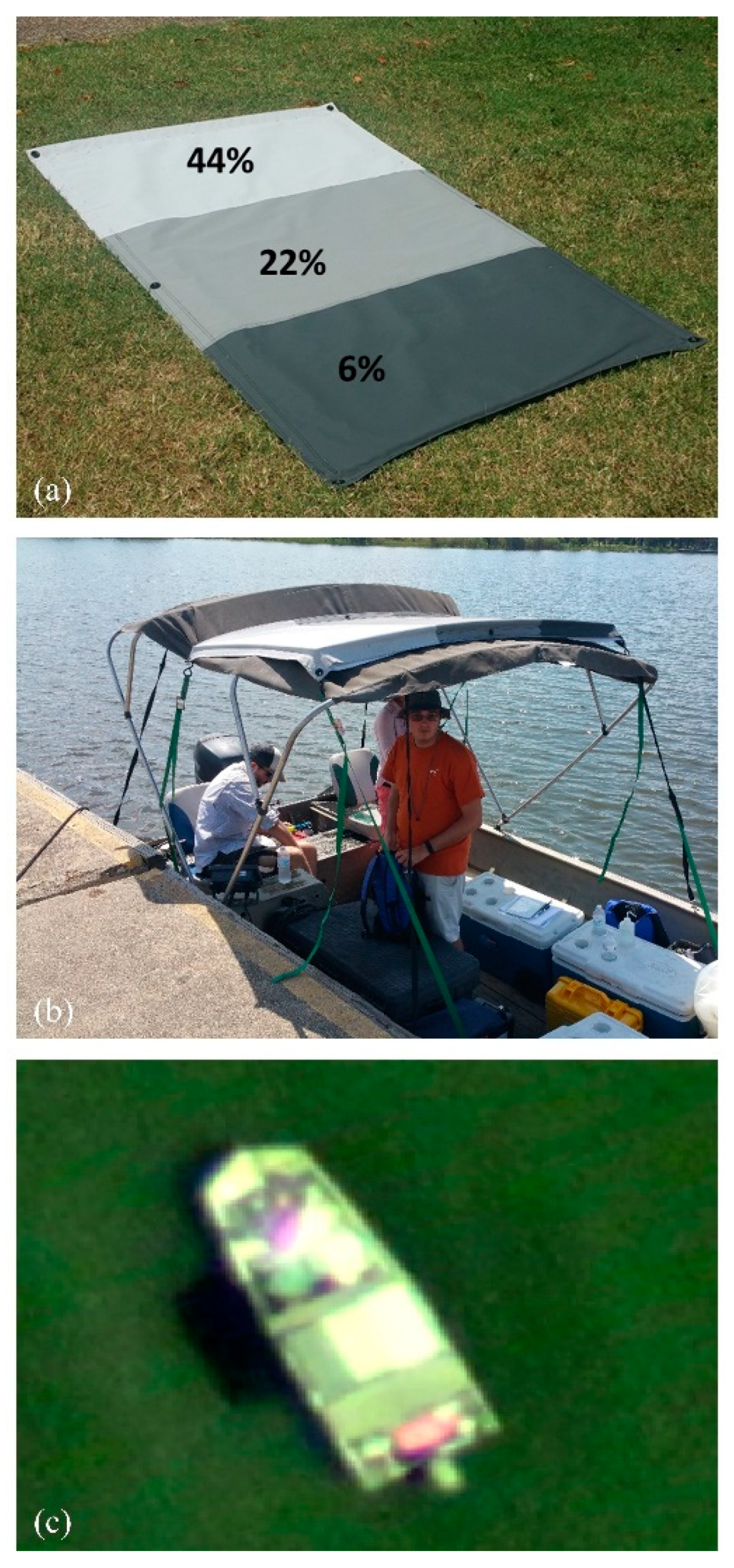
A portable fabric calibration target was constructed to provide a spectrally consistent target in the UAS imagery that could be deployed in both land and water operations. Three spectrally distinct fabric panels were used to balance the amount of equipment carried to the sample sites and the need to quantify any non-linearity in the UAS-spectroradiometer relationship. The darkest panel was a 6% reflectivity value, the medium panel was a 22% reflectivity value, and the lightest panel was a 44% reflectivity value to avoid overexposure of the sensor. Considerations while constructing the target included:
The targets should be large enough to fill the IFOV of multiple sensors and to minimize adjacency effects, yet small enough to be portable and used on a boat.
The targets should lay orthogonal to the sensor.
The targets should have near-Lambertian reflectance properties.
The targets should be durable and washable.
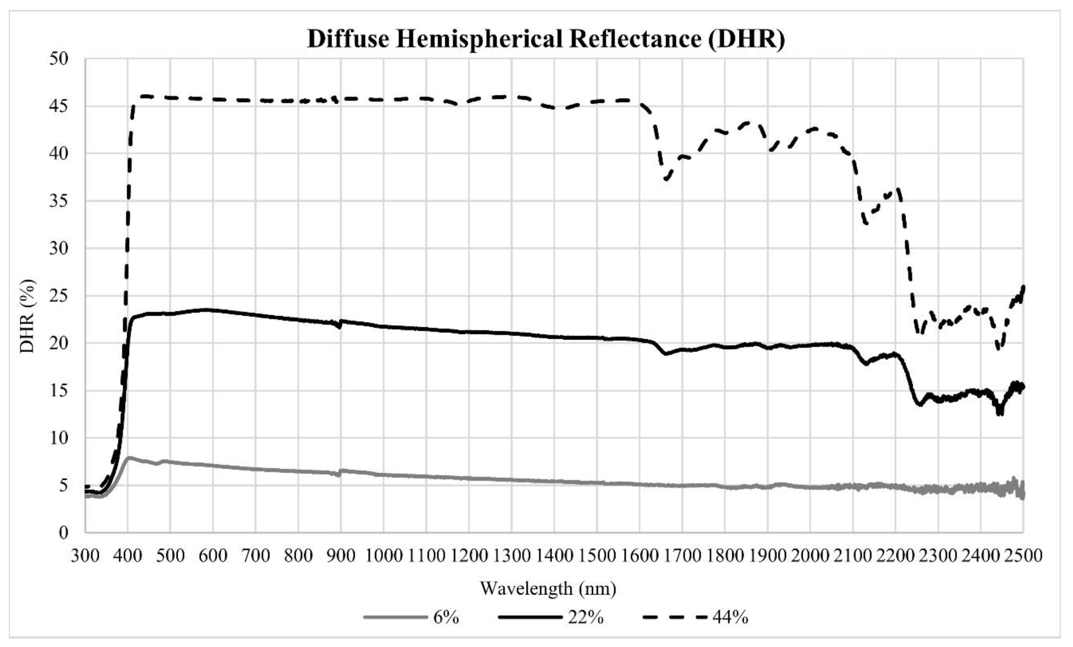
The final calibration target was composed of three 60.96 cm x 1.22 m grey strips of coated Type 822 fabric sewn together using a 2.54 cm overlapping seam and a 5.08 cm folded hem around the perimeter. The Type 822 fabric is a durable, high-strength woven polyester fabric with an Oxford weave that provides near-Lambertian reflectance properties; (Group 8 Technology, Inc., Provo, UT). The coating of the panels was a pigmented acrylic/silicone polymer that was neutral in hue and devoid of spectral content from 420 to 1600 nm. The targets were laboratory-calibrated using a Perkin-Elmer 1050 Spectrophotometer with an integrating sphere so that the band average diffuse hemispherical reflectivity (DHR) of the individual fabric webs were ~6%, ~22%, and ~44% (R +- 0.05R) (
Figure 1;
Table 1).
The panels were sewn onto a larger 1.22 m × 1.83 m piece of uncoated Type 822 fabric. The larger 1.22 m × 1.83 m piece of uncoated Type 822 included a pouch with a Velcro opening and six size-four reinforced clawgrip grommets. The reinforced clawgrip grommets allowed for the tarp to be securely affixed to a boat for water operations. The pouch allowed for an insert (e.g., plywood or other rigid material) so that the calibration target would lie flat on the ground (
Figure 2a) or on the top of a boat canopy (
Figure 2b). The greatest care was taken to prevent creasing while deploying the calibration target.
2.2. Study Site Configurations
2.2.1. Mississippi State University North Farm
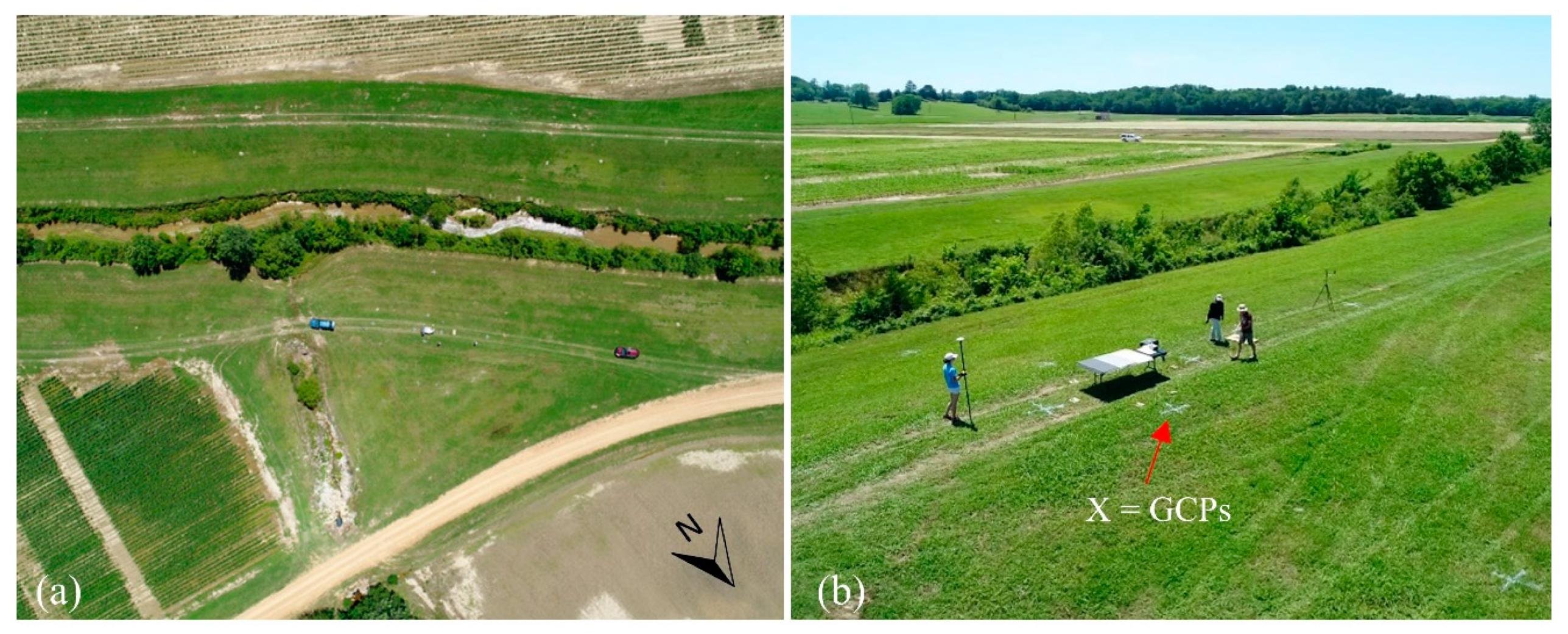
An experiment to quantify the magnitude of atmospheric contributions to UAS imagery at various flight altitudes was conducted at the R. R. Foil Plant Science Research Center (North Farm) on the campus of Mississippi State University (
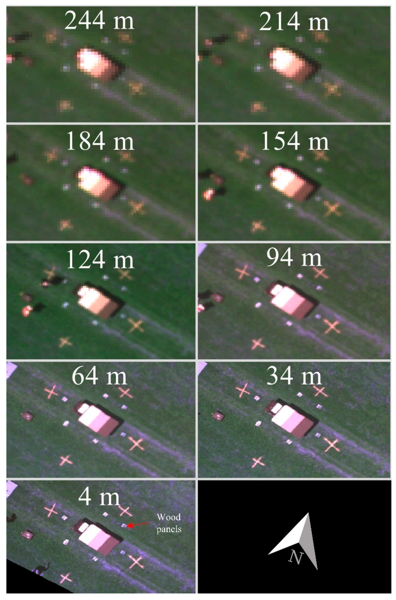
Figure 3). Research teams routinely fly here for precision agriculture applications, and a certificate of authorization (CoA) allowed for an operating altitude of 244 m. A preliminary flight to identify best practices (North Farm 1.0) was conducted. In this flight, it was determined that the calibration reference panels should be placed on a dark table to create a buffer between the tarp and vegetation pixels and ensure the fabric tarp could be pulled tight. It was also determined that 30-meter flight altitude intervals would provide a balance between battery power and the loiter time required at each altitude to collect 30 images of the reference target from each viewing angle. Images collected from seven viewing angles–one set at nadir followed by six additional locations distributed regularly around the calibration–while maintaining a northward orientation allowed for the assessment of the Lambertian properties of the constructed calibration tarp. Conditions with minimal horizontal and vertical winds are preferred to limit the amount of battery required to move between flight altitudes.
North Farm 2.0 (NF2) was conducted on May 2017 during clear sky conditions with light variable winds. The North Farm 2.0 experiment was composed of an X8 octocopter carrying a five-band MicaSense RedEdge® (MicaSense Inc., Seattle, WA, USA) multi-spectral imager with a horizontal resolution of 8 cm when flown 122 m above ground level (AGL) and a footprint of 1280 x 960 pixels. (
Figure 4,
Table 2). The MicaSense camera settings were left fully auto; however, the imagery was radiometrically calibrated and normalized for exposure time and gain following a customized MicaSense RedEdge image processing workflow based on MicaSense image processing scripts explained further in
Section 2.4. The experiment was carried out over a one-hour period from 13:45–14:45 local time (LT). A Windsonde UAS meteorological sensor flown on the UAS recorded consistent relative humidity values of about 45% throughout the flight column.
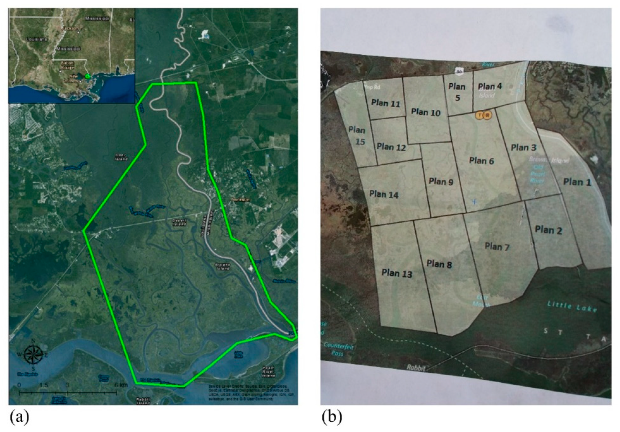
2.2.2. Lower Pearl River
UAS imagery collected over the Lower Pearl River was used to develop and test the simplified ELM radiometric calibration framework. The Lower Pearl River study area spanned a 90 km
2 area over the Lower Pearl River Estuary southeast of Slidell, Louisiana (
Figure 5a). The region is a complex coastal estuary with a mix of low marsh grasses, braided streams, dense forests, man-made structures, and prominent aquatic vegetation. The area is subject to high humidity and sometimes strong sea breeze, often initiating sporadic precipitation events during the warm season. The flight range was limited by the Federal Aviation Administration (FAA) line of sight requirements in place at the time of the study. The changing vegetation, from marsh grass in the southern portion to dense forest in the northern portion, limited the northern extent of flight coverage because line of sight with the UAS became a challenge as vegetation converted to a forested landscape. Accessibility challenges throughout the Lower Pearl River also made it impossible to capture the calibration reference panels in every flight mosaic. Additionally, the north-south orientation of the river network limited the east-west extent of flight coverage to keep the UAS within sight from a boat in the river.
The Lower Pearl River UAS was composed of the Nova Block 3 fixed-wing unmanned aerial vehicle (UAV) flying with a modified Canon EOS Rebel SL1 DSLR camera (
Figure 6,
Table 2). The Nova Block 3 was capable of flying for 80 minutes on a single battery charge. The Canon EOS Rebel SL1 DSLR collected data in three spectral wavebands at a 2.62 cm spatial resolution when flown 122 m above ground level (AGL), with a 24-bit depth, and a footprint of 5184 × 3456 pixels. Only imagery from the August 2015 and December 2015 Lower Pearl River missions was used to develop the study area calibration equations because the calibration reference panels were not constructed until July 2015. Camera settings manually configured for the August 2015 mission were set to an exposure time of 1/4000s, exposure bias of −0.7 step, and focal length of 20 mm. ISO and f-stop were not manually configured and varied across the sampled area. Camera settings for the December 2015 mission were set to an exposure time of 1/4000s, exposure bias of −1.0 step, focal length of 20 mm. Again, ISO and f-stop were not manually configured and varied across the sampled area. It is important to note that the variations in camera settings across the scene were normalized during the flight mosaicking process explained in
Section 2.4.
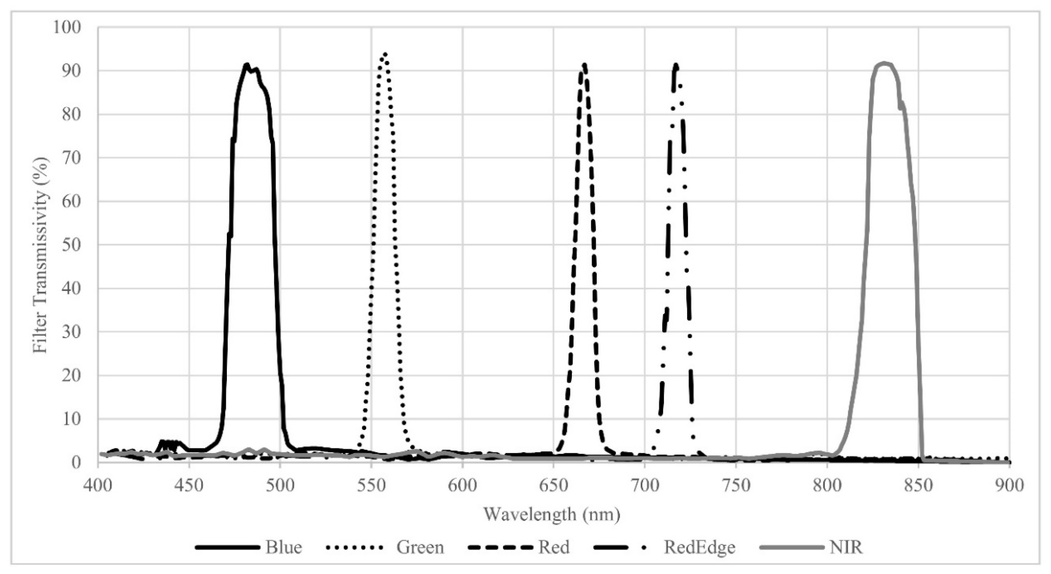
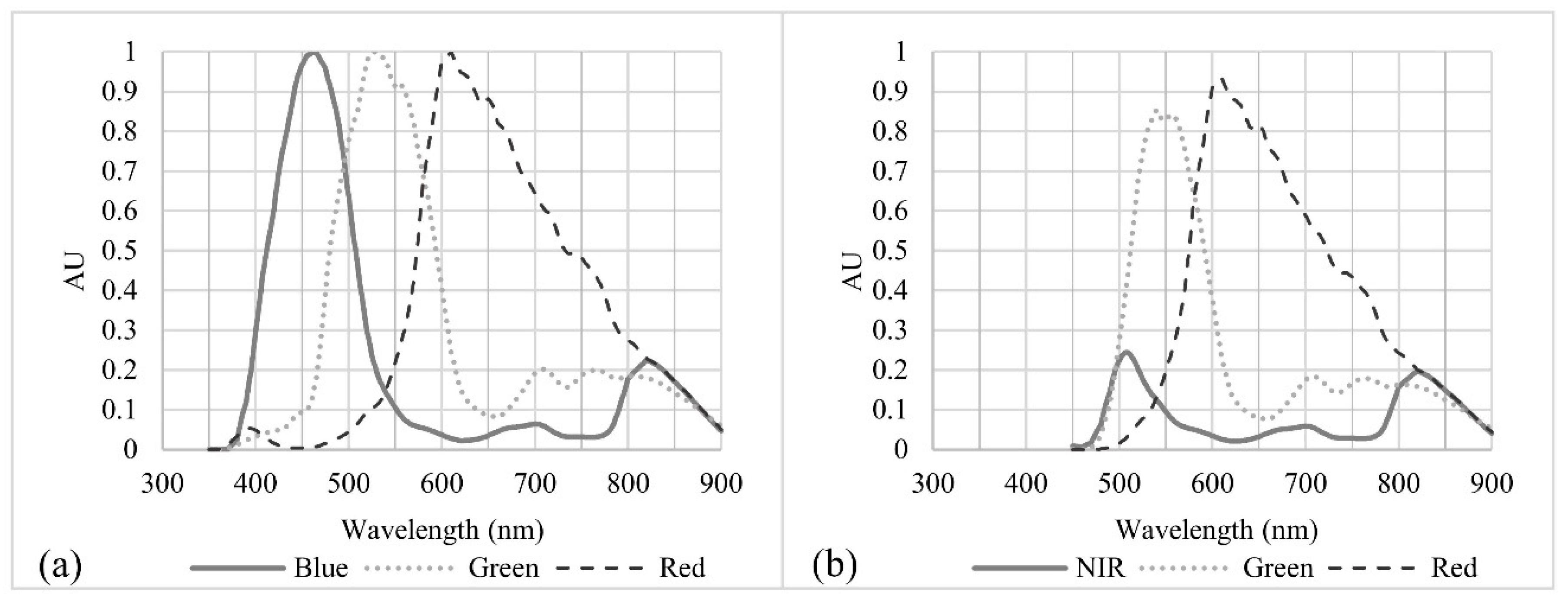
The original camera collected data from 300–1000 nm (
Figure 6a); however, the sensor was retrofitted with a Wratten #12 yellow filter that blocks wavelengths less than 450 nm (
Figure 6b). The purpose of this filter was to convert the blue sensor to a surrogate near-infrared (NIR) sensor. By limiting the response to blue visible wavelengths, the camera was converted to a green-red-NIR colour-infrared (CIR) camera; however, the resulting NIR spectral band had a rather noisy and weak signature.
2.3. Image Collection Procedures
2.3.1. Atmospheric Contribution Experiment (North Farm)
Ground control points (GCPs) were collected using a handheld differential GPS unit (Trimble Geo-7x) from eight locations, marked as “X” in
Figure 3b and
Figure 7, and postprocessed to obtain a 1 cm horizontal accuracy allowing for both georeferencing of the imagery and the creation of polygons over the calibration reference panels that would be used to carefully extract the panel image values of the calibration tarp in each image. Flights were conducted from 4 to 244 m above ground level (AGL) at 30-meter intervals with a constant north heading. A minimum of 30 images of the three greyscale (6%, 22%, 44%) spectrally homogenous reference panels were collected at seven viewing angles, one set at nadir followed by six additional locations distributed regularly around the calibration reference panels, to assess the Lambertian properties of the calibration tarp.
2.3.2. Radiometric Calibration Framework Development (Lower Pearl River)
Flight data collection began in December 2014 with follow-up missions at a near two-month interval (
Table 3). While regular operations began in December 2014, the deployment of the calibration reference panels started during the August 2015 mission. The primary goal of the UAS deployments were to image the greatest aerial extent possible for the mapping of the river system to support the National Weather Service (NWS) Lower Mississippi River Forecast Center (LMRFC) operations; therefore, flight lines varied during each deployment to account for wind direction and to optimize flight time (
Figure 5b). This combination of water-based operations covering a wide range of environmental conditions and variable flight characteristics made for an ideal dataset to develop and examine the performance of a simplified ELM calibration framework for the reduction of atmospheric contributions in UAS imagery and production of scaled remote sensing reflectance imagery with UAS data collected in a rapid deployment configuration with limited site accessibility. However, it is important to note that the framework was tested in a coastal estuary when sky conditions were clear, with scattered clouds, or mostly cloudy; therefore, storms and other atmospheric conditions beyond typical, non-extreme weather conditions were not included in the data.
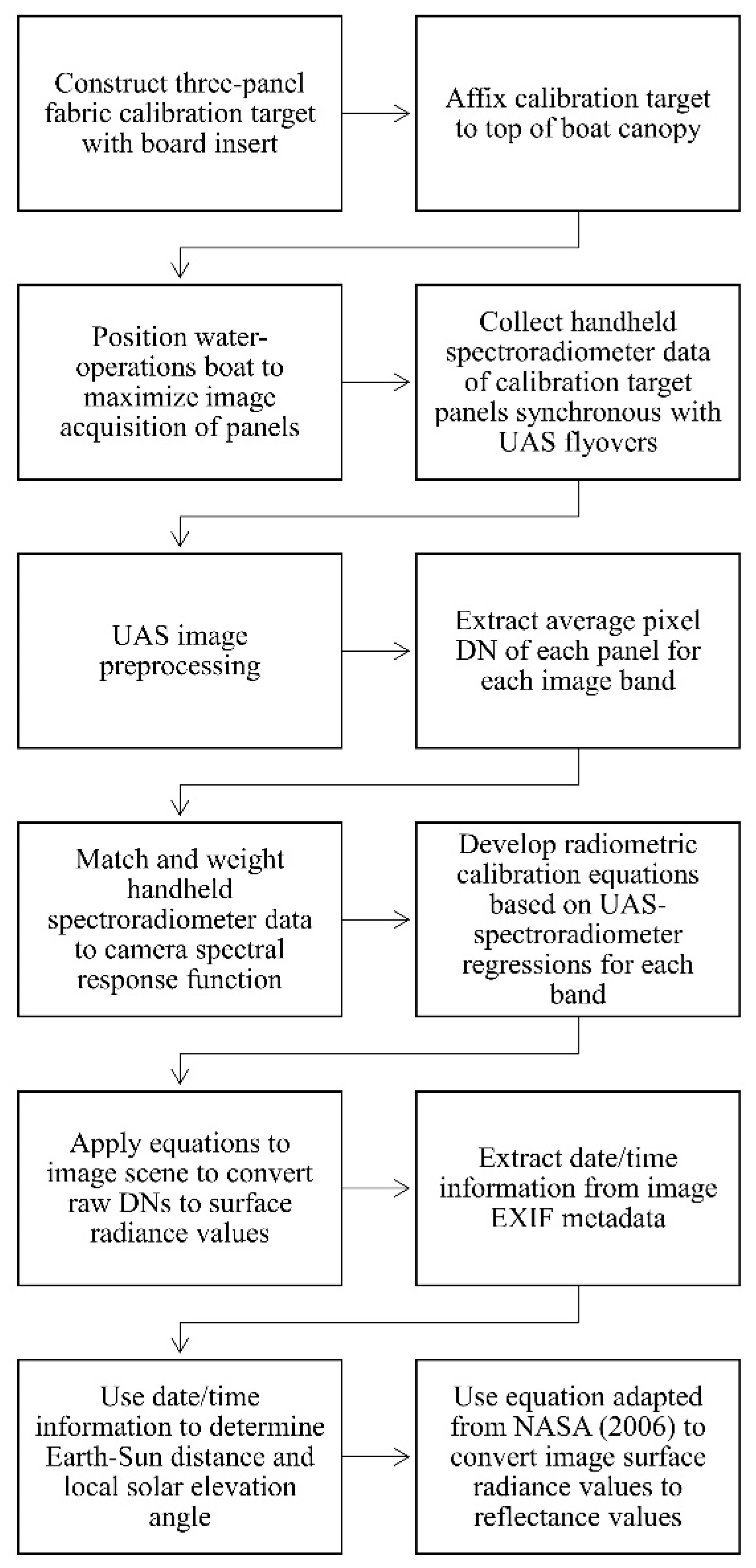
Missions lasted four to six days and imagery was collected between 08:00–16:00 LT with four to five flights per day producing eight to fifteen image acquisition instances of the calibration target per day (32–90 per mission). Regular operations involved two boats, one dedicated to flight operations and the other dedicated to water operations. The flight operations boat was tasked with the flight of the UAS and the download and storage of flight data. The water operations boat worked with the flight operations boat so that in-situ water quality information was collected each time the UAS flew directly overhead the water operations boat. The water operations boat also carried the calibration reference panels and the handheld spectroradiometer. Ground reference data of the calibration reference panels were collected in synchrony with UAS flyovers of the water operations boat using a GER 1500 spectroradiometer (Spectravista Inc., Poughkeepsie, NY, USA). Three GER 1500 spectroradiometer hyperspectral samples of each calibration reference panel were collected and averaged to produce an average spectral signature for each grey value. The workflow from field operations to the final image calibration is summarized in
Figure 8.
2.4. Image Processing
2.4.1. MicaSense RedEdge Imagery (North Farm)
The Geospatial Data Abstraction Library (GDAL) was used to stack the bands and to assign the appropriate WGS84 projection. Minor manual georeferencing corrections were made to ensure the imagery aligned with the ground control points collected by a differential GPS unit. Any images that had obvious artifacts were removed from the analysis. Rectangular shapefiles were manually created and edited to ensure only those pixels representative of the calibration reference panels would be included in the analysis. Imagery was organized by the flight altitude at which the imagery was collected using information from the onboard GPS.
The exposure time was not held constant during the experiment; therefore, as the scene footprint increased with higher flight altitudes, the MicaSense would dynamically adjust exposure settings to compensate for changes in returned signal from new targets in the scene (
Table 4).
These variations were normalized by extracting exposure time and gain information from the image metadata and applying the calibration procedure to the orthomosaics as outlined in the MicaSense tutorial [
53]. This procedure converted the raw pixel values to absolute spectral radiance values (W/m
2/nm/sr). A slight modification was made to the MicaSense postprocessing procedure by removing vignette correction (Equation (1)) because darkening at the corners of the scene had little effect on the pixels representing the calibration tarp at the centre of the scene.
where
is the normalized raw pixel value,
is the normalized black level value,
,
,
are the radiometric calibration coefficients,
is the image exposure time,
is the sensor gain setting,
are the pixel column and row number, and
is the spectral radiance in W/m
2/nm/sr.
All image rasters and panel polygons were projected to an Albers equal-area conic projection (EPSG:5070). This is an imperative step because geographic information systems (GIS) require that data are assigned a relevant projected coordinate system (PCS) for the accurate implementation of spatial analysis tools. The pixel values of each panel were extracted and averaged based on the panel polygon delineation using the ArcGIS 10.3 Spatial Analyst Zonal Statistics tool. The outcome from this analysis was two distributions, one of the uncorrected digital number image values and one of the MicaSense corrected radiance image values.
To further investigate patterns in the MicaSense distributions, a bootstrap resampling technique was applied to the post-processed radiance mean values and the median of the bootstrapped mean values were plotted. This procedure increased the robustness of the sample dataset by reducing the impact of outliers on the plotted median values for each waveband.
2.4.2. Canon EOS Rebel SL1 DSLR Imagery (Lower Pearl River)
Flight mosaics were generated for each mission using a camera alignment technique in the Agisoft Photoscan Pro software. This technique used the orientation of the camera at the time of the image registration and common points in overlapping images to generate tie points to triangulate the camera’s position. A point cloud was generated from this alignment procedure and was examined for any anomalies. The final point cloud was used to generate a mesh on which a GeoTIFF orthomosaic was exported. Variations in camera settings were normalized across the scene in this mosaic processing. All post-processed imagery can be retrieved online (
http://www.gri.msstate.edu/geoportal/).
2.5. Empirical Line Calibration
This section provides a breakdown of the method used to convert the imagery with DN values to calibrated remote sensing reflectance values. The water operations boat would regularly change location after each ground-reference spectroradiometer measurement to reposition to a location that would be orthogonal to a future UAS flight line. During each sampling session, the water operations boat documented the time and location (latitude and longitude) of the sampling site. Upon downloading the UAS imagery, the water operations boat location was manually tagged whenever it was visible in the uncorrected UAS imagery and the calibration reference panels were delineated and stored as rectangular polygons. Because the water operations boat was regularly changing location, the boat location tags included both “sampling” and “in-transit” situations. To prevent inclusion of the “in-transit” locations in the analysis, the UAS DN pixel values were only extracted and averaged across the pixels within each of the delineated calibration reference panels when the manually tagged location information of the boat matched the location information at the time of ground-reference spectroradiometer collection. Hence, the final dataset used for the regression was a series of UAS-weighted ground spectroradiometer radiance values and extracted UAS DN data pairs.
A semi-automated quality control procedure was applied to carefully remove erroneous samples. This procedure included an algorithm that scanned all samples and flagged outliers. Those outliers were then manually interrogated and either retained or discarded. To increase the robustness of the radiometric calibration equations for the study area, the remaining samples from August 2015 and December 2015 missions were combined into a single dataset.
A necessary step was to convert the ground-reference hyperspectral spectroradiometer dataset to the multispectral UAS data by applying the Canon DSLR spectral response function to the handheld GER 1500 spectroradiometer data. This was accomplished by weighting spectroradiometer data values collected during the August 2015 and December 2015 missions with the relative spectral response function of each of the bands of the CIR camera:
where
is the radiance computed for each of the CIR spectral bands,
is the hyperspectral radiance measured using the hand-held spectroradiometer, λi and λj are the lower and upper limits of the bands, and
is the relative spectral response function of the CIR bands [
54,
55].
The limited site accessibility across the Lower Pearl River study area prevented the deployment of the calibration reference panels during every UAS image reconnaissance flight; therefore, image-by-image radiometric calibrations were not possible. While alternatives included radiometric calibrations on a diurnal basis or seasonal basis, exploratory analyses (not shown) indicated that combining data from multiple missions produced more robust calibration equations. This allowed for a single set of radiometric calibration equations to be applied to the full study area independent from sampling time, thereby decreasing the time impacts of the radiometric calibration procedure on rapid UAS deployment operations. Therefore, spectroradiometer–UAS image pairs were combined from multiple flights and conditions to develop robust calibration equations to minimize errors across all UAS missions and atmospheric conditions. Using these spectroradiometer–UAS image pairs, regressions between the UAS weighted spectroradiometer radiance values and the UAS DN values of the calibration reference panels were developed for each spectral band. It is important to note that both radiance and remote sensing reflectance values were computed from the spectroradiometer data; however, spectroradiometer radiance values were used for developing the calibration equations rather than the remote sensing reflectance in regressions so that solar illumination could be applied later to the radiance data to obtain more accurate remote sensing reflectance relative to when the image acquisition took place. Two-thirds of the available site data from August 2015 and December 2015 were randomly selected and used to develop the calibration equations. The remaining third of data was used to verify the performance of the calibration equations. The calibration equations were then applied to each associated image band across the full mission mosaics.
Once the imagery was calibrated and the UAS DNs were converted to radiance, the imagery was normalized for illumination by converting from radiance to remote sensing reflectance in each waveband using the following equation adapted from NASA [
56]:
where
is the spectral radiance, d is the Earth–Sun distance in astronomical units,
is the local solar elevation angle [which is equivalent to 90° minus the local solar zenith angle (
)], and
is the average spectral global irradiance at the surface for each band based on the American Society for Testing and Materials (ASTM) G-173-03 direct normal spectra.
This method of conducting the radiometric calibration for obtaining radiance, then the use of average surface irradiance and the solar illumination geometry for obtaining remote sensing reflectance was selected because the solar illumination conditions in past and future UAS applications will be different than the solar illumination conditions experienced during the development of the calibration equations. For example, some constraints of the current study included: (1) UAS images were collected in some areas of the Lower Pearl River estuary that were inaccessible preventing the deployment of the calibration reference panels; (2) illumination conditions changed between UAS flights conducted at different times of the day and during different times of the year; and (3) three flight campaigns (December 2014, March 2015, and May 2015) were conducted prior to the development and deployment of the calibration reference panels. Therefore, this was the best approach for reducing errors in that previously collected imagery. Furthermore, rather than developing new calibration equations for each time of the year to account for the prevailing illumination conditions, this approach allows for the application of the calibration equations to the data from the imaging sensor throughout the year to obtain radiance first, and then use the solar irradiance of the corresponding day to produce precise remote sensing reflectance imagery.
Performance of the calibration equations was assessed using the normalized root mean square error (NRMSE), the normalized mean absolute error (NMAE), goodness of fit (R2), and a Mann–Whitney U test. The normalized NRMSE and NMAE were calculated by dividing the root mean square error (RMSE) and the mean absolute error (MAE) by the range of the observed spectroradiometer data. This normalization facilitates the comparison of results with future datasets of different scales. The Mann–Whitney U test is a nonparametric test that assesses whether the distributions of observed and predicted datasets are equal; therefore, the Mann–Whitney U test was used to test the null hypothesis (Ho) that the distribution of the predicted and actual datasets are equal.
3. Results and Discussion
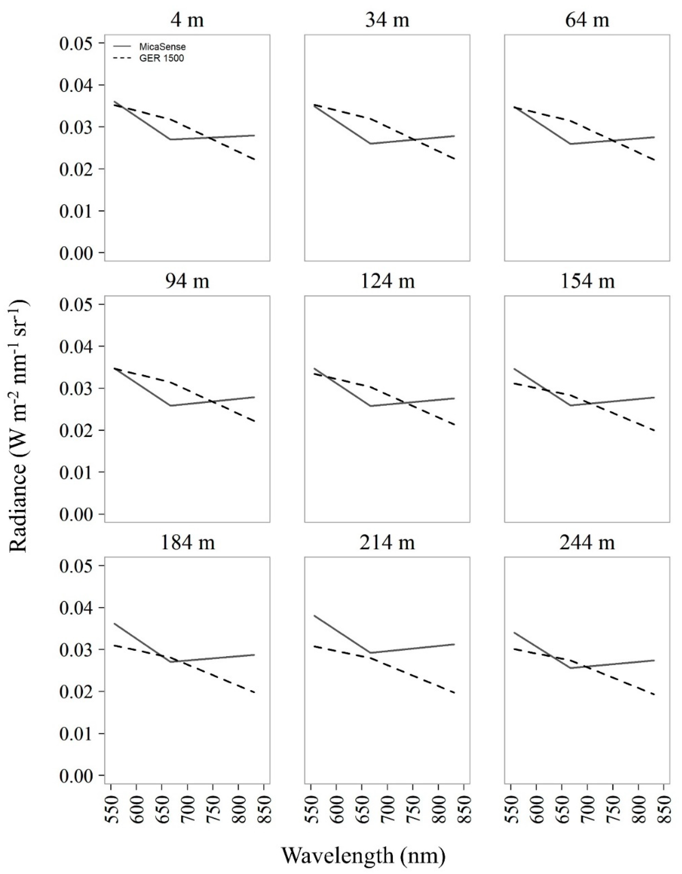
From the NF2 experiment, it was clear that an ELM radiometric calibration would be required for the Lower Pearl River UAS imagery. This is illustrated by comparing the GER 1500 ground spectroradiometer radiance values with the airborne green, red, and NIR MicaSense radiance values at each flight altitude (
Figure 9). There was an important and clear increasing trend in atmospheric contributions to the UAS imagery, especially at flight altitudes higher than 124 m. Compared to the ground-based spectroradiometer radiance values, the MicaSense green and NIR radiance values returned greater signal to the imager at all flight altitudes. The MicaSense red band did not show radiance values as high as green and NIR bands because this specific band had a lower spectral response than is shown in the spectral response function from the manufacturer in
Figure 4, indicating that it needs calibration. This points to the fact that coefficients derived in the lab and applied to this imagery in Equation (1) may not perform with the same accuracy in the field [
57]. Nevertheless, the consistently higher radiance in the green band with increased altitude confirms that the imagery was impacted by atmospheric contributions. In addition to atmospheric scattering, there were challenges in obtaining representative spectral information from the 22% and 44% calibration reference panels because of saturated pixels (i.e., DN values >=65,520). This oversaturation was caused by the automated MicaSense exposure and ISO settings and it reduced the effectiveness of the prescribed MicaSense radiometric calibration procedures. Overall, the outcomes from the North Farm experiment suggested that an ELM radiometric calibration was required prior to obtaining biophysical information from the Lower Pearl River UAS imagery in order to develop new calibration coefficients to adjust for: (1) errors emanating from applying lab-derived coefficients to field imagery, (2) changes in sensor spectral response that occur after laboratory calibrations, and (3) atmospheric contributions to the imagery.
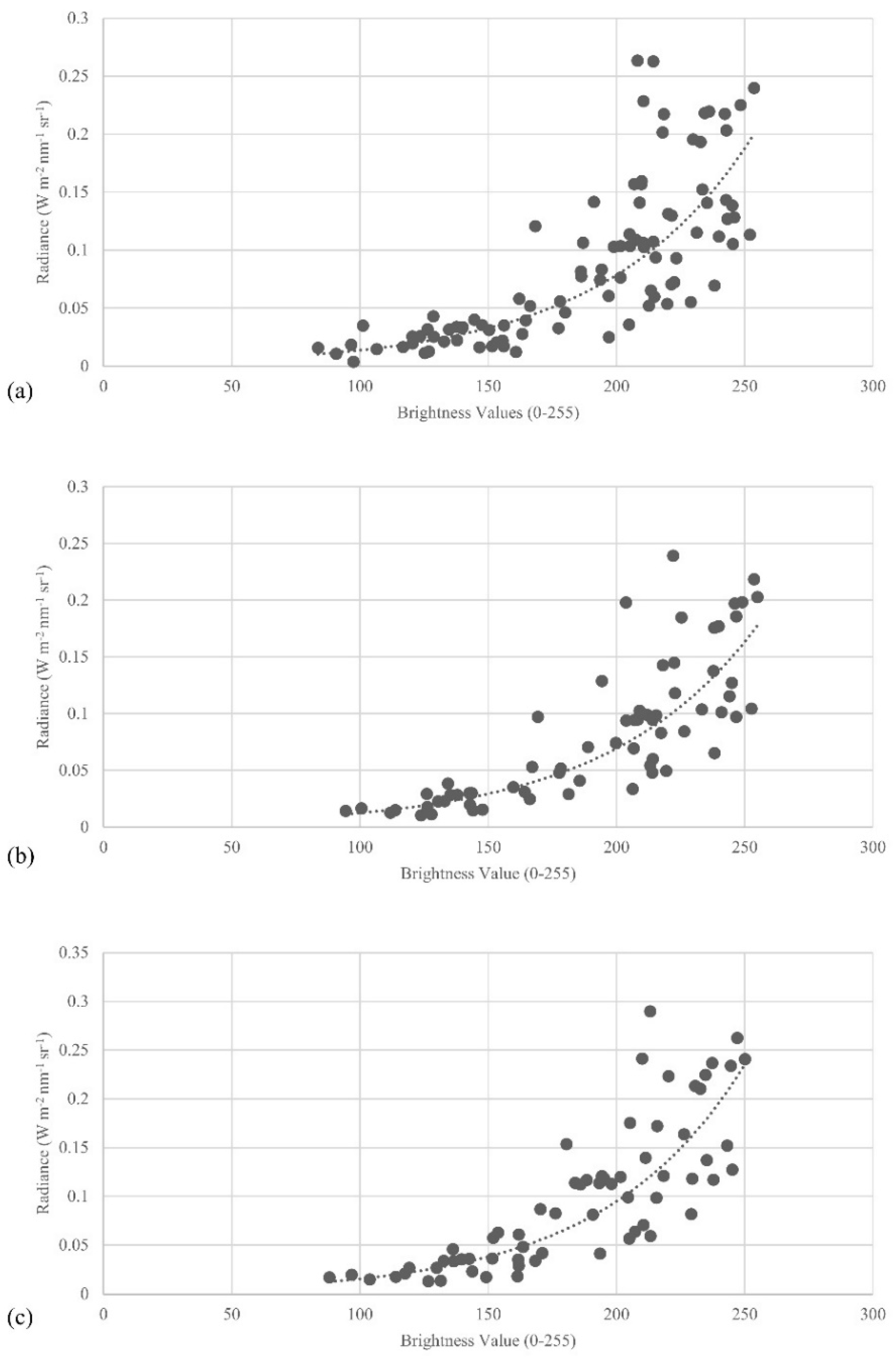
The Canon DSLR flown in the Lower Pearl River missions exhibited an exponential relationship between the raw Canon DNs and the GER 1500 ground spectroradiometer measured radiance values (
Figure 10). These exponential relationships agree with past research [
40,
44,
45,
48]. The goodness of fit for each band (R
2 green = 0.77, R
2 red = 0.79, R
2 nir = 0.77) is relatively high considering the current study was conducted over water and incorporated spectroradiometer–UAS DN pairs that spanned multiple missions to develop the radiometric calibration equations. Normalized RMSE and normalized MAE are also within acceptable ranges for each spectral band (
Table 5). The Mann–Whitney U test results were not significant, indicating that the distribution of the predicted and measured datasets for all spectral bands are not significantly different. This is consistent with the outcomes from Wang and Myint [
40] confirming that the simplified ELM radiometric calibration framework developed in the current study effectively reduces external factors influencing UAS imagery, including atmospheric contributions, while also producing scaled remote sensing reflectance imagery for all Lower Pearl River missions.
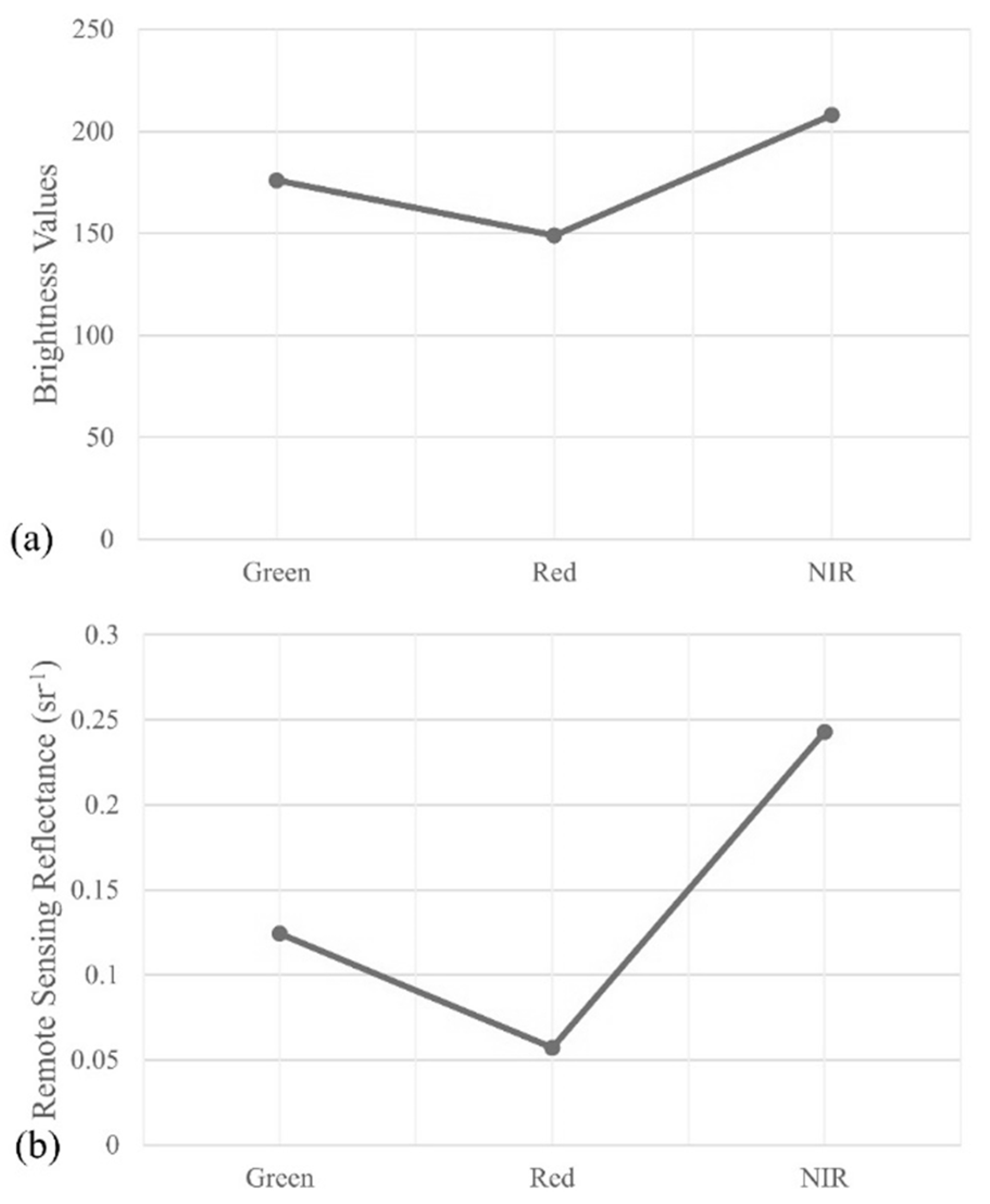
To further illustrate the performance of the presented ELM radiometric calibration framework, 2000 vegetation pixels were randomly selected and their median spectral response was plotted for the August 2015 mission imagery (
Figure 11). Healthy vegetation should return a much stronger NIR signal than green and red. However, the brightness values in green and red bands were quite high, as observed in
Figure 11a. These high values in the green and red bands are due to atmospheric contributions to the imagery and errors emanating from inherent differences in the spectral responses of the sensor bands (as shown in
Figure 6). After applying the calibration equations, the green and red signals decreased resulting in a typical vegetation spectral response. The further dividing of solar irradiance to obtain remote sensing reflectance helped to minimize additional error due to variations in solar conditions throughout the image collection period (
Figure 11b). A unique aspect of the proposed framework is this separation of radiance calibration and normalization of solar irradiance which allowed for the correction of any imagery collected with the same Canon DSLR camera independent from the time of collection; therefore, this framework also allows for the application of the calibration equations to imagery collected at a different time.
If irradiance can be measured during every UAS flight, then a more proper conversion of radiance to reflectance should be the goal of every study to produce the most accurate conversion from radiance to remote sensing reflectance. In the event that these irradiance measurements are unavailable due to study site accessibility or missing reference panels during data acquisition, then this framework offers a viable alternative for reducing errors in UAS imagery. In the current study, the development of these calibration equations using numerous sampling areas across multiple missions and under various environmental conditions created robust operational calibration equations. While this framework produced a lower goodness-of-fit value compared to recent land-based studies, the calibration equations better represent the varied conditions of the study area and are effective in reducing atmospheric contributions and other external factors across the full study area without requiring ground-reference spectroradiometer data in every flight mosaic. However, it is imperative to acknowledge that some error will persist because the calibration equations were developed using information collected under a variety of conditions, such as changes in illumination conditions across the scene due to scattered clouds.
Consistent illumination conditions across the flight mosaics were one of the greatest challenges, because it was rare that the sampling coincided with an entirely clear-sky day in the coastal estuary environment. This created local illumination variations that led to situations where the UAS flyover of the boat and the time of the ground reference spectroradiometer sampling occurred under sunny conditions while some portions of the scene were influenced by cloud shadows when sampled by the UAS. Some UAS flyovers of the boat and ground reference spectroradiometer sampling occurred under a cloud shadow, so those cloudy local illumination effects were quantified to some degree by the calibration equation. Ideally, however, the future integration of automated techniques to normalize cloud shadow effects by collecting upward irradiance data onboard the UAS during flights would help to overcome the cloud shadow effects.
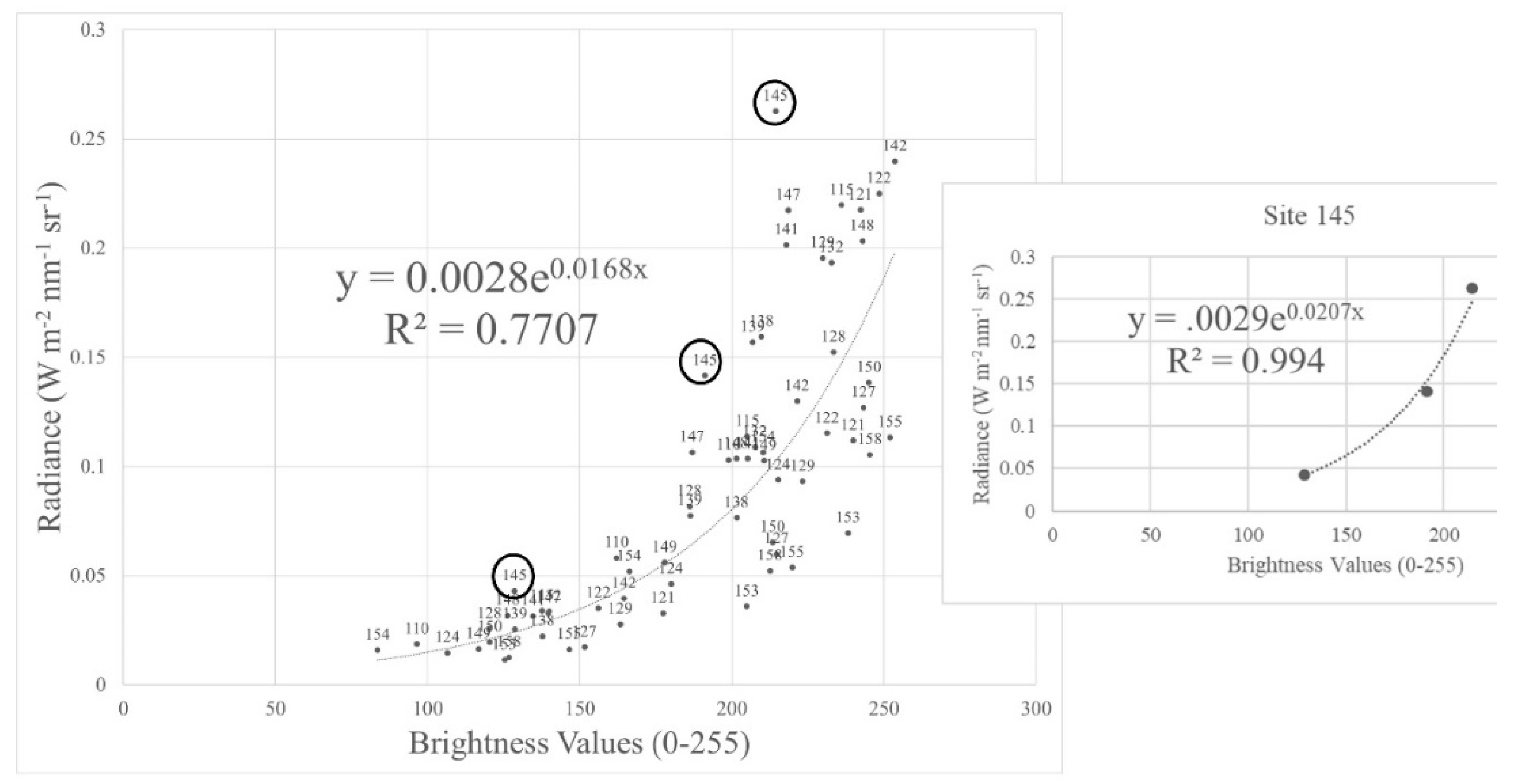
It is likely that the accuracy of the Lower Pearl River radiometric calibrations would be further improved with the incorporation of a bidirectional reflectance distribution function (BRDF) correction [
58,
59]. Furthermore, an image-by-image calibration could potentially help acquire the level of accuracy identified in previous UAS-based ELM radiometric calibration studies (
Figure 12); however, image-by-image calibration equations were not feasible in this study because the UAS was often flying over inaccessible areas (e.g., forested wetlands or salt marshes) and it was not possible to deploy the calibration reference panels nor collect hand-held spectroradiometer data in these areas.
This points to the importance of identifying mission spectral accuracy requirements prior to the execution of any UAS field operation. If greater spectral accuracy is required, then image-by-image calibrations may be preferred; however, image-by-image calibrations will only be applicable to missions sampling a relatively small area. A recent approach by Mafanya et al. [
45] proposes an effective method for improving calibration accuracy for larger scenes by implementing a statistical assessment to ensure the scene being corrected is not significantly different than the scene from which the calibration equations were developed. While shown to be effective for land-based studies, future research is required to assess the performance of this approach in water-based studies. Furthermore, it remains uncertain how corrections should be applied to scenes significantly different than the scene from which the calibration equations were developed. Hence, the proposed ELM radiometric calibration framework and subsequent calculation of remote sensing reflectance offers a method for developing and applying calibration equations to large study areas independent from diurnal and seasonal variations. The proposed framework will be best adapted in studies with limited site accessibility or in rapid response configurations where temporal constraints limit the ability to deploy and sample calibration reference panels within the area of interest.
4. Conclusions
The objective of the current study was to develop a simplified empirical line method (ELM) radiometric calibration framework for the reduction of atmospheric contributions in unmanned aerial system (UAS) imagery and for the production of scaled remote sensing reflectance imagery for UAS operations with limited site accessibility and data acquisition time constraints. Experiments were conducted at the R. R. Foil Plant Science Research Center (North Farm) on the campus of Mississippi State University to quantify the degree to which atmospheric contributions implicate UAS imagery. Imagery collected over the Mississippi State University North Farm experimental agricultural facility indicated that atmospheric contributions to UAS imagery have the greatest impacts on shorter wavelength bands (e.g., green band), and there is a gradual increase in these atmospheric contributions within a relatively small flight column (4-244 m above ground level). A simplified ELM radiometric calibration was proposed to reduce the impacts of these atmospheric contributions on UAS imagery. Unique to the current study was the water-based nature of regular UAS imagery reconnaissance missions. This required the modification of existing UAS radiometric calibration frameworks and led to the development of a rapidly deployable calibration target and a cost- and time-effective radiometric calibration framework for correcting UAS imagery across various applications.
Results agreed with previous studies that an exponential relationship exists between the UAS recorded DNs and spectroradiometer radiance values. Calibration equations developed from these ground spectroradiometer–UAS relationships performed well, indicating that the proposed radiometric calibration framework effectively reduces atmospheric contributions in UAS imagery. A benefit of the proposed framework is that the calibration equations were developed independently from the solar illumination normalization so that the calibration equations can be applied to any past or future imagery collected over the study area with the same imaging sensor. This greatly extends the capacity to improve UAS image accuracy in a variety of complex and rapid response sampling conditions where highly controlled calibration target deployment and intensive radiometric calibration procedures are not feasible. As such, the current study helps pave the way for future research exploring UAS-based remote sensing applications. The figures presented can be used as reference to understand the varied implications of atmospheric contributions on UAS imagery relative to flight altitude; however, additional experiments under various conditions would be useful to further examine these atmospheric contributions to UAS imagery across additional locations and conditions. Follow-up experiments involving a hyperspectral spectral imaging sensor, advanced on-board meteorological instrumentation, and higher flight altitudes could further distinguish planetary boundary layer factors impacting UAS imagery.

 ,
, 


