
Efficient Reactive Obstacle Avoidance Using Spirals for Escape
by
 , , , and
Fábio Azevedo
1,2,* ,
,
Jaime S. Cardoso
1,3 ,
,
André Ferreira
2,
Tiago Fernandes
2,†,
Miguel Moreira
2 and
Luís Campos
4 1
Electrical and Computing Engineering Department, FEUP, University of Porto, 4200-465 Porto, Portugal
2
Beyond Vision, 3830-352 Ílhavo, Portugal
3
Institute for Systems and Computer Engineering, Technology and Science, 4200-465 Porto, Portugal
4
PDMFC, 1300-609 Lisbon, Portugal
*
Author to whom correspondence should be addressed.
†
Current address: Critical Techworks, 4000-091 Porto, Portugal.
Drones 2021, 5(2), 51; https://0-doi-org.brum.beds.ac.uk/10.3390/drones5020051
Submission received: 30 April 2021
/
Revised: 26 May 2021
/
Accepted: 2 June 2021
/
Published: 7 June 2021
(This article belongs to the Special Issue Feature Papers of Drones)
Abstract
:The usage of unmanned aerial vehicles (UAV) has increased in recent years and new application scenarios have emerged. Some of them involve tasks that require a high degree of autonomy, leading to increasingly complex systems. In order for a robot to be autonomous, it requires appropriate perception sensors that interpret the environment and enable the correct execution of the main task of mobile robotics: navigation. In the case of UAVs, flying at low altitude greatly increases the probability of encountering obstacles, so they need a fast, simple, and robust method of collision avoidance. This work covers the problem of navigation in unknown scenarios by implementing a simple, yet robust, environment-reactive approach. The implementation is done with both CPU and GPU map representations to allow wider coverage of possible applications. This method searches for obstacles that cross a cylindrical safety volume, and selects an escape point from a spiral for avoiding the obstacle. The algorithm is able to successfully navigate in complex scenarios, using both a high and low-power computer, typically found aboard UAVs, relying only on a depth camera with a limited FOV and range. Depending on the configuration, the algorithm can process point clouds at nearly 40 Hz in Jetson Nano, while checking for threats at 10 kHz. Some preliminary tests were conducted with real-world scenarios, showing both the advantages and limitations of CPU and GPU-based methodologies.
1. Introduction
In recent years, there have been research efforts in the field of aerial robotics that have led to a broader range of application scenarios [1]. This growing number of applications is closely related to the continuous change in the research focus, which tends to approach higher-level tasks (such as navigation and task planning, paying attention to visual odometry, localisation and mapping) [2].
Due to their success, the use of multirotor unmanned aerial vehicles (UAV) is migrating from an isolated robotics’ research topic to a trendy tool [3] that supports several applications and enables the possibility of new ones. The general interest in this type of robot stems from their main characteristics: high manoeuvrability, hover ability, and a reasonable payload–size ratio. At the current stage of development, UAVs can be used for search and rescue missions, surveillance and inspection, mapping, among others [4], carrying task-specific sensors (for example, cameras, optical sensors, and laser scanners).
The main objective of using drones is to support or enable the execution of tasks that usually rely on human labour, while reducing risks and operational costs [3,5]. However, this usually implies a high degree of autonomy of the UAV, which significantly increases the complexity of the system and requires the use of perception sensors and algorithms to interpret them and generate appropriate control outputs. Navigation in complex and harsh environments can be challenging, which implies the need for an obstacle detection and collision avoidance module.
Obstacle detection is divided into three main steps: (1) data acquisition from the perception sensors; (2) data treatment and representation in memory; (3) and, finally, the detection of threatening obstacles. The first module is responsible for successfully communicating with the sensors and reading data from them. In the second step, the data treatment may involve some pre-filtering (such as limiting the accepted range of a point cloud), and their representation may also require some data clustering to reduce the memory requirements. Detection of the potentially risky obstacles depends on their good representation and benefits from clustering, as it reduces the computational power required to verify whether the obstacle interferes with the desired path. However, when clustering, special care has to be taken to avoid losing meaningful environmental features.
Collision avoidance is responsible for calculating an avoidance trajectory in a minimal time window. It needs to be fast enough to generate a solution without colliding with obstacles. Therefore, it works as a bridge to produce navigation control commands from the perceived obstacles in the surrounding environment.
As mentioned earlier, operating in harsh and confined environments increases the perception requirements and control complexity. UAVs must be aware of the obstacles and avoid collisions, even if this means neglecting their primary goal for self-security reasons.
Some approaches deal well with the task of path planning in known scenarios, such as PRM [6] or RRT [7]. However, when working outdoors, the assumption of known scenarios rarely holds [8], so an algorithm capable of reacting quickly enough to changes in the environment to avoid crashing is needed. Works such as that in [5] attempts to address this by using a 360-degree long-range 3D light detection and ranging (LiDAR) to perceive the environment, using Octomaps [9] to store and process large point clouds.
This work aims to contribute with a reactive approach to the collision avoidance methods, while keeping its procedure robust and straightforward. Despite the focus on the collision avoidance layer, obstacle detection is also part of the study, as the avoidance procedure clearly depends on it. The main challenge that arises as a limitation for the developed work is the use of only one depth camera with a very limited field-of-view (FOV) as a perception sensor, with a range of up to 10 m. This requires the algorithm to be extremely fast, from data acquisition to control commands generation. Adding to this, is the requirement to be able to run in a resource-constrained UAV on-board computer. To exploit the implementation possibilities in a real scenario, both a CPU and a GPU solution are developed, being tested, evaluated, and validated in a simulation environment.
The contributions of this article are then fourfold:
- The development of an efficient and simple but robust method for reacting and avoiding collisions with static or slow-moving obstacles that are not known beforehand;
- The implementation of the method for both CPU and GPU, evidencing their advantages and drawbacks. The evaluation is done with different hardware setups and conditions;
- Consideration of the environment perception as part of the method, since it is one of the main bases for the avoidance procedure;
- Usage of a spiral to search for escape point candidates. Starting from the obstacle’s centre, the spiral provides a quasi-optimal solution to avoid the obstacle in terms of deviation from the original path. The first valid point is the one that deviates the least from the original path, providing a collision-free operation.
The remaining article is organised as follows: Section 2 provides some insight about literature related to the reactive collision avoidance topic; Section 3 presents some background on the frameworks used to implement the methodologies detailed in Section 4. The results are in Section 5 and their discussion in Section 6. The final conclusions and future steps envisioned are in Section 7.
2. Related Work
This section presents some of the existing works that use a reactive collision avoidance approach, mainly using point-cloud-based methods.
The addition of a third degree of freedom in trajectory planning for obstacles avoidance significantly increases the complexity of the task. To overcome this problem, some literature works [10,11,12] decompose the problem into a 2D analysis using 2.5D maps. However, these maps result from projecting the 3D environment onto multiple planes and are particularly useful for robots with predominant movement in 2D planes. When the robot has the freedom to navigate in 3D space, some authors [13,14] use adaptive path planners based on traditional approaches, like A* [15], D* lite [16], PRM [6], or RRT [7]. Besides their high computational cost, these types of approaches generally have the disadvantage of always computing a collision-free path to the desired final position, which can be a waste of resources in an unknown or continuously changing environment.
Given this, the use of a reactive approach is preferable to deal with the unknown, since the key idea is to navigate in complex environments using simple approaches to locally avoid the most threatening obstacles. Examples of sensors that directly generate point clouds are LiDARs, depth cameras or, more recently, event cameras (through the accumulation of events over time). A more in-depth analysis on the usage of LiDAR or camera-based approaches is done in [17].
2.1. Reactive Approaches
Merz and Kendoul [18] presented a LiDAR-based collision avoidance solution for helicopters in structure inspection scenarios. They use only a 2D LiDAR and apply the pirouette descent and waggle cruise flight modes to correctly map the 3D environment by sweeping the sensor. This approach relies heavily on the accurate estimation of the vehicle’s position to properly detect obstacles. No processing time analysis performed, but the vehicle is able to perform uninterrupted flights while avoiding the obstacles, providing a real-time solution.
Hrabar, in [19] also presented a reactive approach to collision avoidance. Whenever an obstacle is detected in the planned path, the algorithm spawns an elliptical search zone, orthogonal to the vehicle-goal straight path, to find potential escape points. Those candidate escape points are considered valid only if there is a collision-free path from the vehicle to them, and from them to a predefined distance in the direction of the destination point. If no valid points are found, the ellipse expands up to 100 m, needing the pilot intervention if no valid solution is found. The safety volume is composed of spheres spaced in a way that approximate a cylinder. The escape points search typically took 17.7 ms (10 m ellipse) but can go up to 260 ms in the worst-case scenario, using a Bkd-tree search approach. Both a stereo vision and LiDAR-based approach were tested (isolated and combined), with the best results obtained when using the LiDAR-only system, even using a 15-m range, in contrast to the 35-meter range of the stereo system.
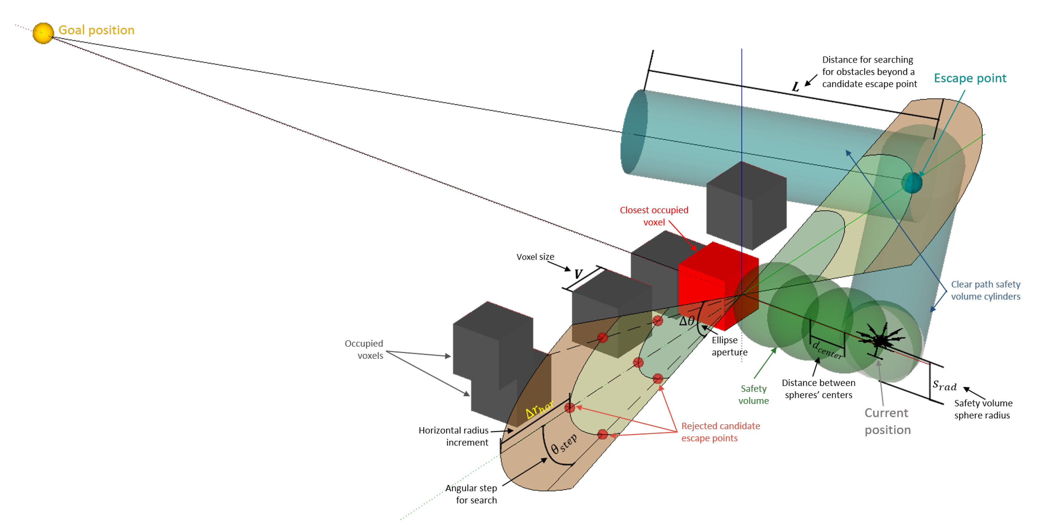
In [5], Hrabar’s work is studied and extended, using a LiDAR sensor with 360-degree coverage and a range of up to 100 m (but using only 40 m). The main contributions to the previous solution were (1) limiting the search area of escape points to favour horizontal movements and prevent navigation manoeuvres with the sensor’s blind spots, (2) a dynamic safety volume that increases with the vehicle’s speed, (3) a local minima escape procedure if no valid escape points are found, and (4) a limited search space of 20 m around the UAV’s position. The algorithm’s procedure is depicted in Figure 1. The obstacle’s search took, on average, 1 ms to be processed, while the escape point calculations required 0.97 ms in a desktop computer (760 obstacle points). The tests with the UAV on-board computer had only 83 obstacle points, resulting in 0.4 ms for obstacle search and 8.63 ms to calculate escape points, clearly showing a performance dependence on the number of obstacles found.
An alternative real-time approach proposed by Vanneste et al. [20] consists of an extrapolation of the 2D VFH+ [21] to 3D using a 2D polar histogram of the environment. The histogram is constructed based on the Octomap voxels, representing the azimuth and elevation angles between the robot position and the evaluated voxel. The generation of a new robot motion takes on average only 326 s. The main drawback of this method is the number of tuning parameters needed, depending on the application.
Other existing methods take into account the existence of known UAVs in the surroundings for the collision avoidance trajectory. Alejo et al. [22] proposed an indoor method based on optimal reciprocal collision avoidance (ORCA), where each UAV takes responsibility in the process of avoiding others’ trajectories. All the planning and trajectory generation is done by a simple central computer that knows the initial planned trajectories of each UAV (pre-inserted), their positions at every moment (using a VICON localisation system), and the parameters of the UAVs’ model. Static objects are also previously known, since they are imported from a mesh file. The planning is done in the velocity space, and the vehicles have to react when the current velocities differ from the desired. Due to the existence of a centralised control and lack of perception on-board the UAVs, this method is not suitable for direct application in an outdoor scenario.
The works of [23,24] deal with collision avoidance for aircraft sharing the same space and static obstacles. In [23], they assume that UAVs know the position, speed, and heading of neighbouring aircraft, within a given sensing range. The optimal path is based on essential visibility graphs (EVG) dynamically updated when new UAVs or obstacles are detected. When in a collision course, the UAVs are forced to follow the right of way rules to comply with the existing aviation regulations. Du et al. approach [24] relies on dynamically updated potential fields with an attractive force to the original planned path, and repulsive forces to uncooperative UAVs. They also assume the timely and correct detection of the latter, as well as an accurate inference of their position and speed. Despite being valid methods for avoiding collisions with other UAVs, they both present results for detection and avoidance in the range of hundreds of meters.
The approaches in [22,23] are mainly focused on the reaction to the presence of other moving agents. There are also some works that try to deal with the short-range collision eminence with dynamic objects at low altitudes, like birds or thrown balls. These objects either have an unpredictable reaction to the eminence of collision, or are simply unable to take action for avoiding it. [3] uses a monocular camera to detect potential dynamic obstacles based on a deep learning approach. DroNet [25] also uses a deep learning solution to enable drone navigation by training the network with car driving videos. Similarly to [22], the processing is all done by an external computer that sends commands to the drone. When an obstacle crosses its path, the drone simply stops. A successful implementation to avoid dynamic obstacles as well is presented in [26], where the authors use an event camera and calculate an avoidance command depending on the direction and speed of the obstacles, by combining attractive and repulsive forces (similarly to [24]). The calculations are based on the accumulation of events over a time window and take 3.5 ms from acquisition to command generation.
2.2. Analysis
After examining some 3D reactive collision avoidance methods, it becomes apparent that it is a complex task that usually requires significant processing power. Some approaches try to deal with this issue by reducing the search space or clustering the data. However, the resources required to perform these actions are not considered in the final evaluation of the algorithm. The reconfiguration of the search space may take some time, depending on the size of the working map. The insertion of the point cloud is also a very critical step, as it can be of considerable size and should be processed as quickly as possible due to the urgency of the collision avoidance task. However, existing methods tend to neglect this step as part of the avoidance procedure.
Another very important feature that needs special care is the navigation to unknown areas, especially when the perception sensor is not able to map them while moving, e.g., moving vertically and having only a static 2D laser in the horizontal. Navigating into the blind spot of the sensor is undesirable due to the risk of collision with undetected obstacles. In the case of depth cameras, the effect of limited range and field-of-view (FOV) can be minimised by rotating the UAV to the desired point before moving linearly.
3. Background
3.1. Octomap
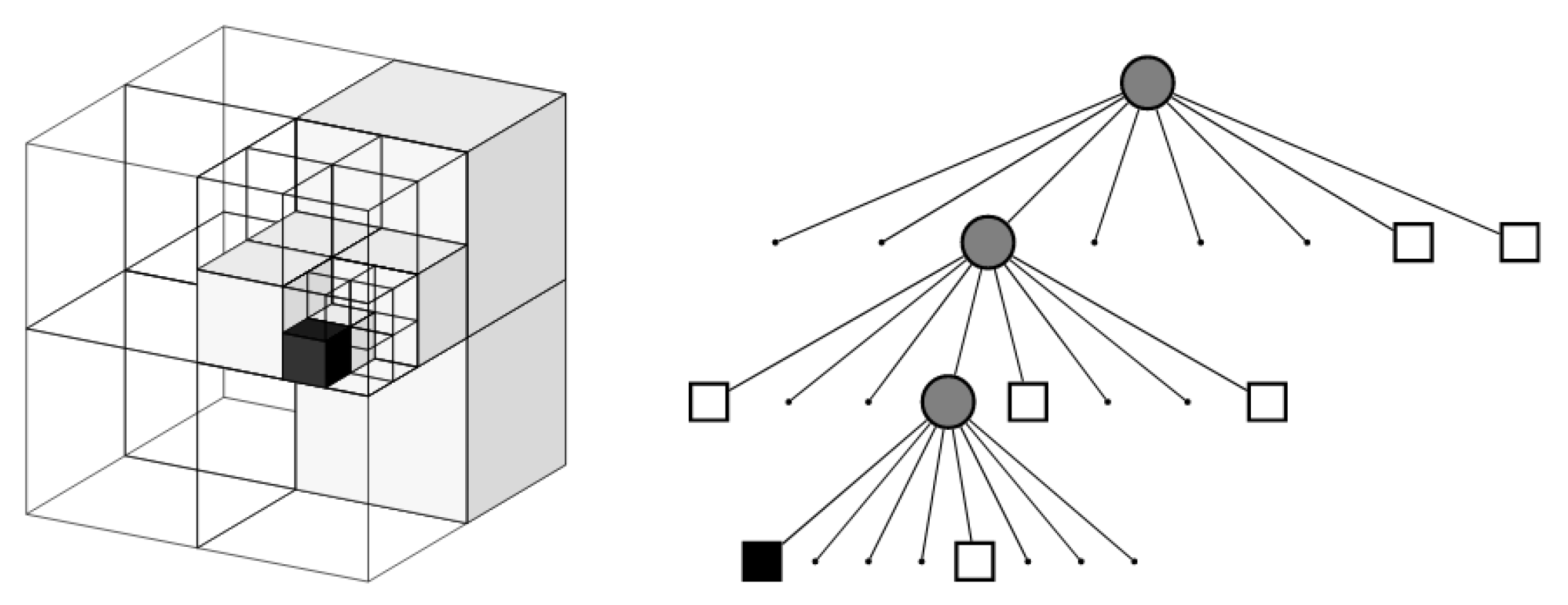
The Octomap framework [9] provides an efficient way to represent 3D environments using an occupancy grid based on the octree data structure. The octree provides an hierarchical structure containing multiple nodes, called voxels, that correspond to cubic structures in the 3D space. Each voxel may contain either 8 or 0 child voxels. If all 8 child voxels have the same state (free or occupied), their representation is reduced to the parent voxel only; otherwise, the 8-voxel representation is kept (Figure 2).
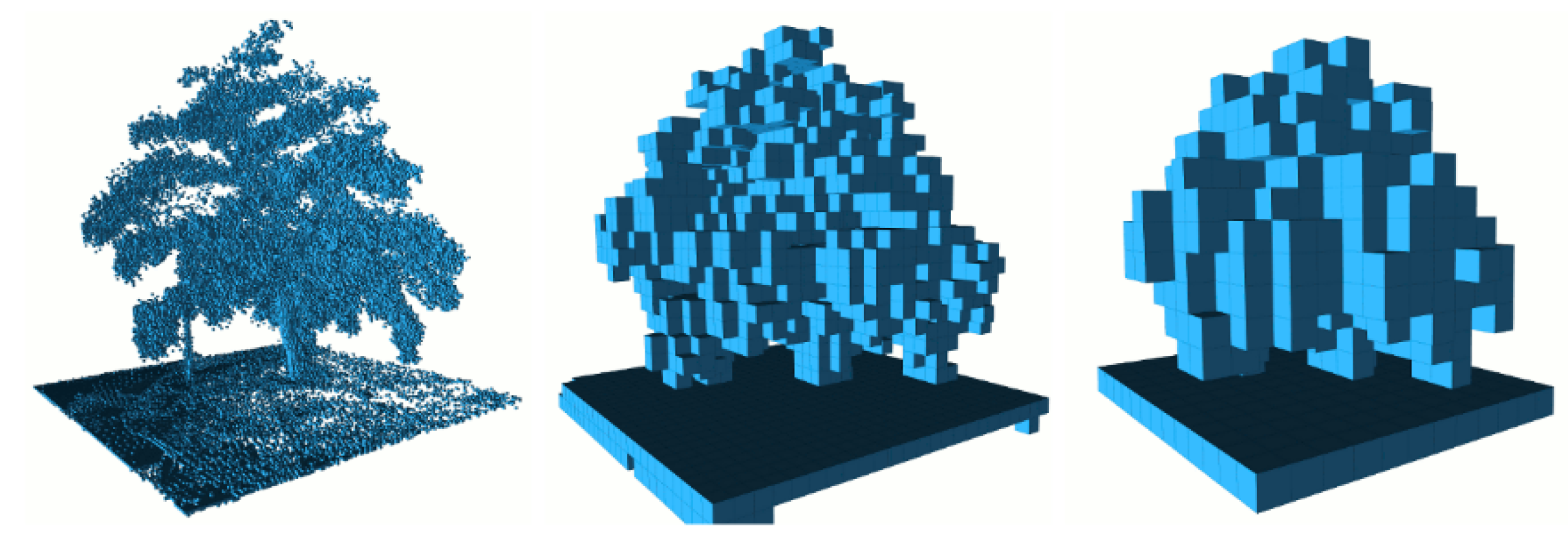
The base resolution of the octree and the number of layers determine the precision and size of the voxels and allow the environment to be represented at the desired resolution (Figure 3). The Octomap framework does not contain direct information about the voxel 3D location. It is defined only for the root voxel, being the location of the child nodes obtained by descending the layers of the tree. Each leaf of the tree corresponds to a cubic structure in the 3D space. The deeper the layer, the smaller the cube and, therefore, more resolution of the map.
Due to the noise and uncertainties of the sensors, the Octomap’s leaves have a probabilistic number of occupancy to represent the environment. Applying a defined threshold, the voxels can be classified as free or occupied. Unseen voxels have an unknown state. When using this map representation for navigation, there are two possible approaches: avoiding the occupied voxels or following the free voxels.
3.2. GPU-Voxels
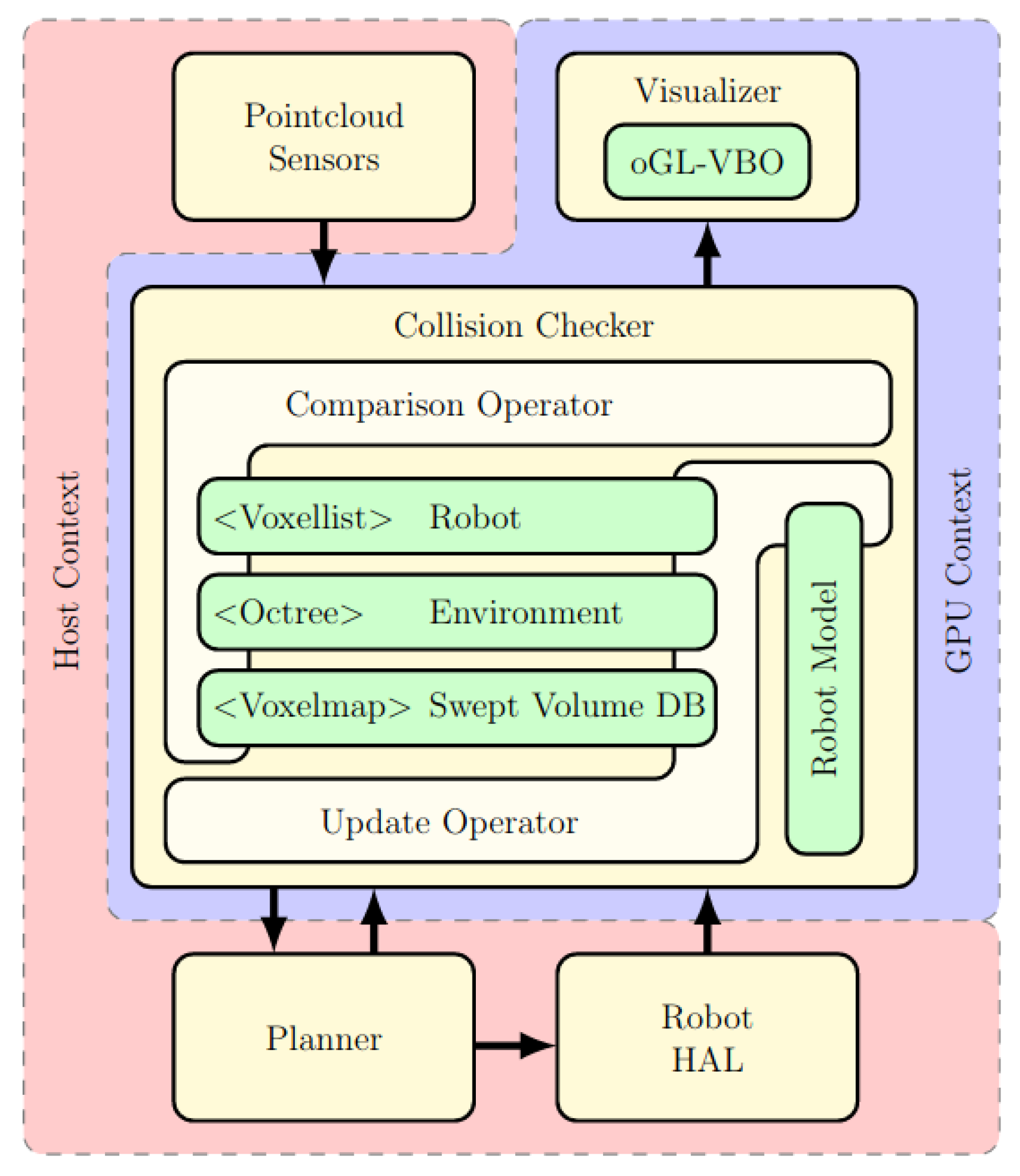
GPU-Voxels [27] is very similar to the Octomap framework. It outperforms Octomaps by exploring the highly-parallelised capabilities of a GPU, instead of being only CPU-based, with a task division as depicted in Figure 4.
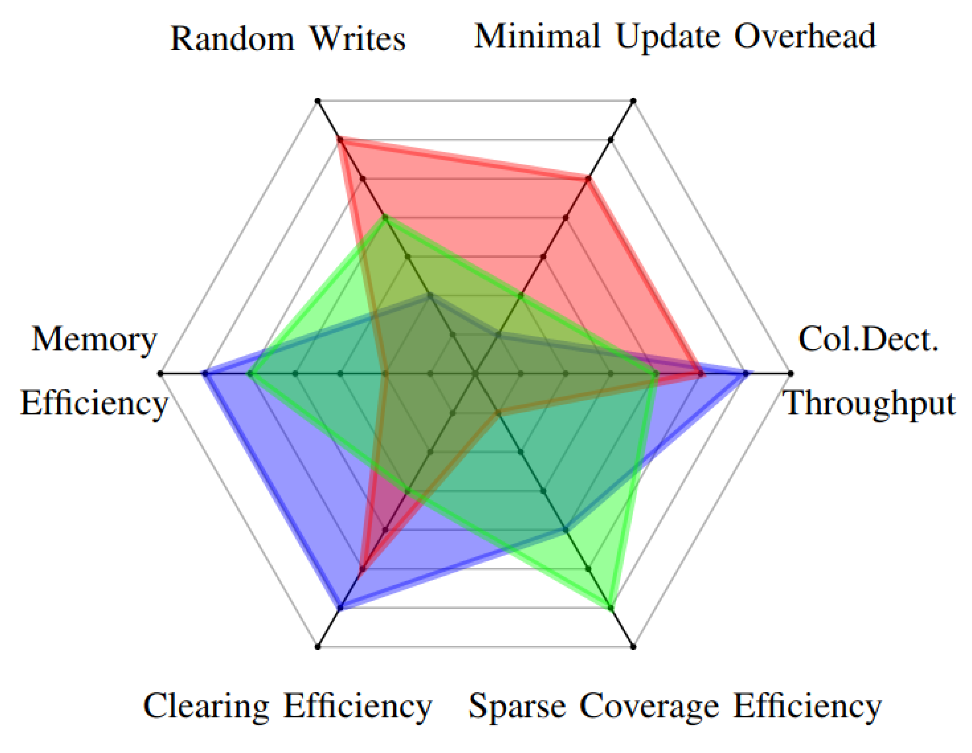
There are currently three implemented storage data structures: Voxel Map, Octree and Voxel Lists. Depending on the use case, the structure shall be chosen accordingly (Figure 5). In the insertion of new point clouds, the Voxel Map representation provides an additional distance map, where each location is updated with the distance to the nearest occupied voxel.
Voxel Map storage provides a very fast interface to update the voxels and get useful measurements for collision detection. However, it allocates a complete map even to unknown areas, making it less memory-efficient. In contrast, Voxel Lists have good memory efficiency while maintaining collision detection speed by storing data in lists of relevant data only and not dealing with empty voxels. The Octree representation is a more balanced structure that is especially beneficial in sparse environments due to its hierarchical nature, which has already been described in Section 3.1.
4. Materials and Methods
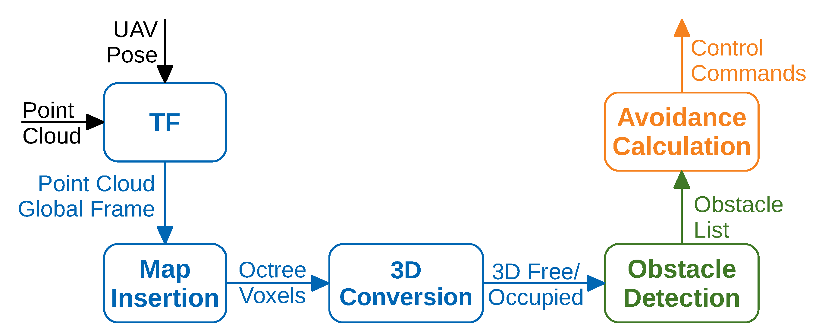
This section describes the work developed. This work covers the entire pipeline of a point-cloud-based collision avoidance algorithm, starting with the insertion of the perceived data (Figure 6).
Data received from sensors must be mapped into a global reference frame before being inserted into the map representation to ensure coherence of the data over time. In general, planners need the input data mapped into a 3D space. Therefore, after an octree representation of the environment, both free and occupied voxels are mapped into the 3D Euclidean space representing the input for the obstacle detection phase. From the obstacle list, the avoidance path calculation generates the control commands for the UAV. The low-level specifics of UAV control are beyond the scope of this work.
In the implementation details described here, the collision avoidance pipeline consists of three stages: the insertion of the point cloud and environment representation (in blue, Figure 6), the search and detection of obstacles (in green), and the final computation of the collision avoidance path (in orange). All phases were implemented using ROS nodelets [28,29,30] associated to the same handler to reduce both memory usage (zero-copy between nodes) and processing time, since the data does not need to be serialised and deserialised in the publish–subscribe mechanism.
The method for reactive collision avoidance was implemented to work, and being compared, in both CPU and GPU. Due to the difference in architectures, some procedures differ between implementations. Therefore, the full pipeline of the method is first presented for the CPU implementation, being then pointed out and described the differences for the GPU.
4.1. CPU Approach
4.1.1. Point Cloud Insertion
In this work, the input point cloud is directly provided by a depth camera. In the CPU-based approach, the algorithm uses Octomap [9] to represent the environment.
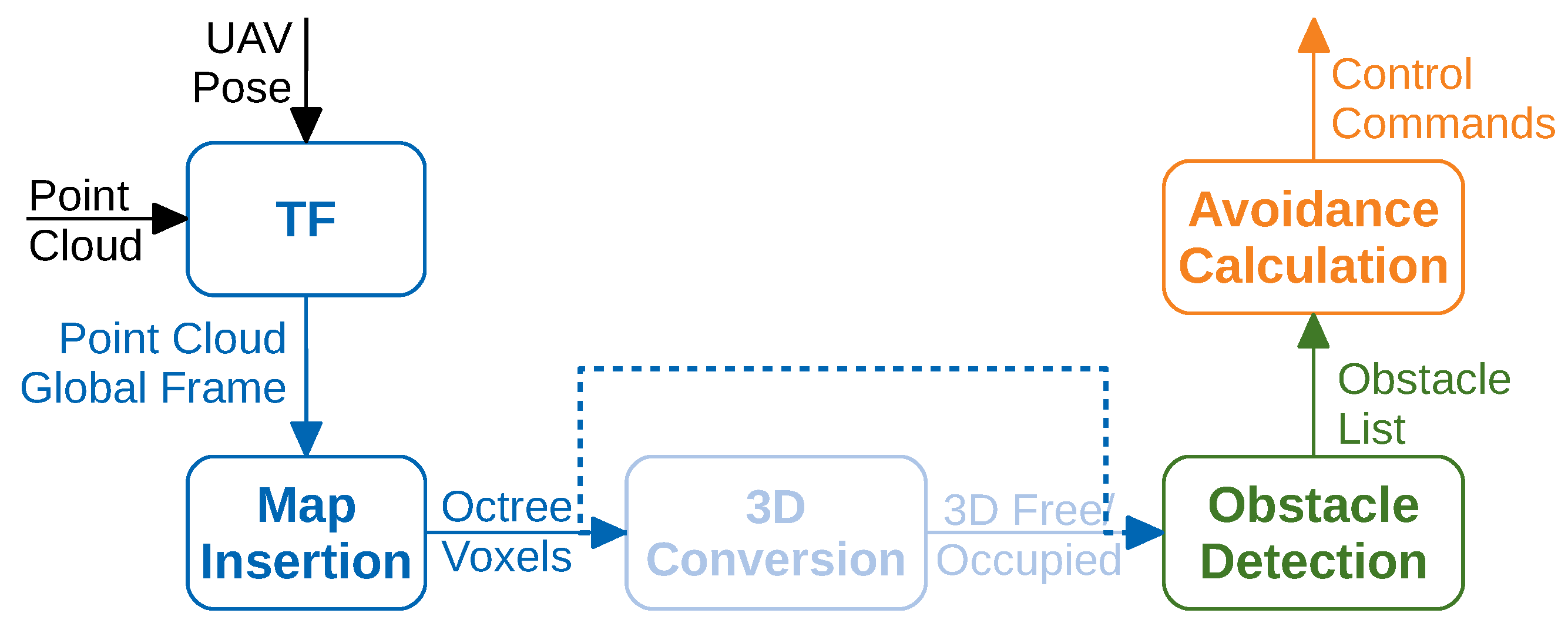
After the point cloud is adequately transformed into the global frame, it is inserted into the octree, updating the corresponding nodes. To speed up the processing, the map insertion is stopped at this phase, neglecting the conversion of occupied nodes in the 3D Euclidean space, as depicted in Figure 7. Instead, the obstacle detection stage directly accesses the octree keys, by inverse converting the 3D points in the evaluation only when absolutely necessary.
4.1.2. Obstacle Detection
The obstacle detection method is based on the works [5,19] by implementing a cylindrical safety volume to check threatening objects. However, the CPU and GPU-based solutions differ in the cylinder approximation strategy.
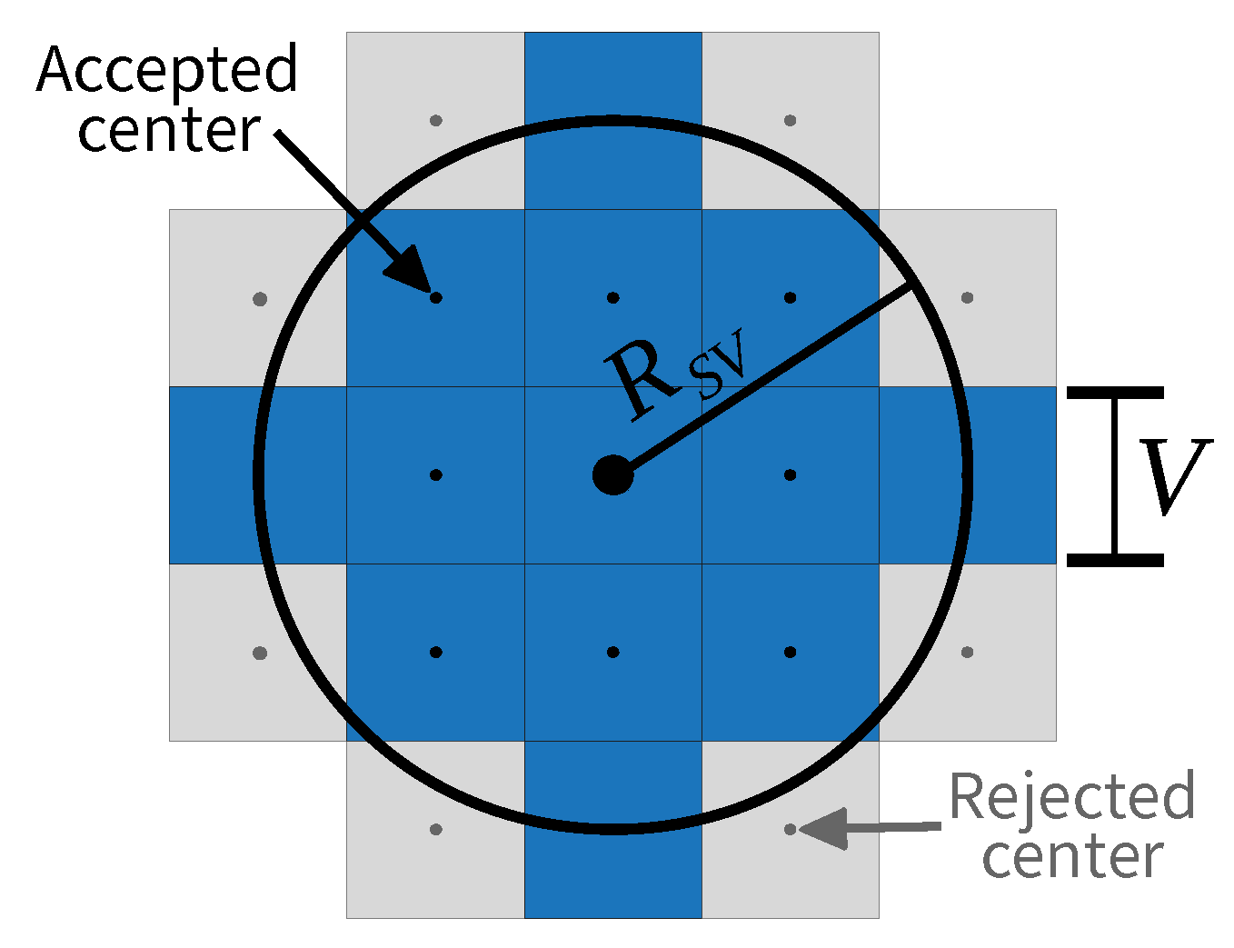
To take advantage of the very efficient raycast implementation of Octomap, the cylinder approximation was performed by firing n rays along the drone-waypoint direction with a length L. Figure 8 shows an orthogonal cross-section of the approximation process.
The number of rays fired depends on the desired safety radius and the voxel size V. The rays are parallel and spaced by V to ensure the coverage of all internal voxels in the desired safety volume. On the external part, the cylinder volume is not fully covered, but the tolerance can be neglected since the motion of the vehicle will cover it at a later time. In a centre calculation with i horizontal steps and j vertical steps, the centres are accepted to fire a ray only if the following condition is satisfied:
Being the current UAV’s position and the goal position, the normalised direction is given by and the ray’s starting positions (after passing the validation step of Equation (1)) are given by:
The search with ray firing begins from the centre of the safety volume up to the radius limit and always returns the nearest obstacle that intersects the volume. The used cylinder length L is calculated by the minimum value between a predefined search range and the distance to the waypoint plus a safety distance:
4.1.3. Avoidance Calculation
This stage is only triggered when an obstacle is found and uses the closest object for reacting to the existence of obstructing obstacles.
The process of avoiding an obstacle consists of searching an escape point, similarly to [5,19], but this work uses an Archimedean spiral () rather than an ellipse. The spiral was chosen since it provides a continuous function that moves away from the origin with a linear angle growth. This provides an approach that tries to search for avoidance paths, giving preference to those that less affect the original desired path.
Whenever an obstacle is found, the algorithm starts the search for valid escape points using the spiral presented in Figure 9. The spiral is centred in the obstacle , following a horizontal direction that is orthogonal to the drone-waypoint direction . Therefore, the candidates’ coordinates will be calculated as follows:
If , the candidate escape point is rejected, and the algorithm continues the search. This approach tries to prevent the avoidance of obstacles from below and gives preference to horizontal avoidance or altitude increasing since the probability of finding obstacles tends to increase with the decrease in altitude. In the implemented approach, the arc length used was and the winding separation .
With the increasing of the spiral radius, the angle step needed to ensure a constant decreases. Using an iterative search approach, the following angle can be approximated based on the previous by solving:
Considering a valid escape point , the algorithm applies the procedure described in Section 4.1.2 and Section 4.2.2 for detecting obstacles for CPU or GPU, according to the setup chosen. This stage tries to verify if the path is clear from the current UAV position to the escape point, and from it to the final goal point (along a predefined length, for example, 10 m). If the escape point is valid, it is sent as an intermediate goal point to the UAV; otherwise, the algorithm moves to the next candidate until it finds a solution or reaches a maximum number of iterations. The scenario depicted in Figure 1 helps in understanding this method, in which case the spiral replaces the ellipse.
4.2. GPU Approach
4.2.1. Point Cloud Insertion
Instead of Octomaps, the GPU-approach uses GPU-Voxels [27] with the Voxel Map storage method. Despite the large memory requirements, the Voxel Map storage method was chosen as it provides a faster update while keeping the collision detection throughput high (see Figure 5). It also generates a distance map that is updated on insertion, having the distance to the closest occupied voxel at a certain point. This feature is desirable to the obstacle detection stage since it keeps the searching process simple.
4.2.2. Obstacle Detection
Taking advantage of the distance map provided by the Voxel Map storage method, the process of searching for obstacles is the same as in [5,19], where the cylindrical shape is approximated by a set of spheres (Figure 10).
The maximum allowed sphere distance is defined by:
This value is used to calculate the number of needed spheres:
Then the sphere distance is recalculated to keep a constant displacement:
Using the normalised displacement vector , the spheres’ centres are calculated as:
The obstacle’s search is then simply getting the distance to the closest occupied voxel in the GPU-Voxel distance map and verify if it is smaller than . If yes, the correspondent occupied voxel position is returned. To optimise the process, the search begins in the drone’s centre and expands until L, returning immediately if an obstacle is found, ignoring the verification of farther spheres.
4.2.3. Avoidance Calculation
Unlike the previous stages, the avoidance path calculation is common to the CPU and GPU approaches.
4.3. UAV Control
In this work, only a depth camera will be used to perceive the environment. Since it has a very limited FOV, when an obstacle is detected, the UAV controller stops the motion and aligns its heading to the direction of the next waypoint before resuming the motion. This is necessary to ensure a collision-free operation without navigating blindly in unknown areas.
In case no viable alternate path is found after the iteration limit, a recovery procedure has been implemented that instructs the drone to navigate to the previous waypoint and to try to navigate to the problematic area again, but now with more knowledge about the environment. To enable this approach, the UAV keeps a record of the waypoints used throughout the process. This is also of interest for return to launch manoeuvres in complex environments since a viable path (although in reverse) was already found, depending on moving obstacles.
4.4. Summary
Figure 11 presents the algorithm’s state flowchart to help to understand the steps presented in this section.
The grey box contains the elements related to the UAV control. Whenever a Final Waypoint (desired position) is received, the drone aligns its heading and moves towards it. At each iteration, it verifies if the waypoint was reached, and stops the movement whenever it reaches the final waypoint. A waypoint is considered either a goal position received externally or an escape point from the avoidance procedure.
In parallel with the control, the depth point cloud is stored using the Octomaps or GPU-Voxels framework (blue box). Combining this information with the UAV’s pose and waypoint, the algorithm keeps searching for potentially threatening obstacles (green box), triggering the avoidance path calculation (orange box) if any is found. If the algorithm is not able to get a valid avoidance path, the UAV navigates to the previous waypoint and then resumes its operation towards the Final Waypoint. Otherwise, an escape point is used to avoid the obstacle before going to the final position.
5. Results
This section presents the main results of the different components of this work. The evaluation of the method was divided into two phases: the first was an offline test using Gazebo simulator, and the second was a preliminary trial using the real hardware in a real scenario. The Gazebo simulator is a primary tool used by ROS for robotic simulations in both academic and professional environments. Since it was developed from its genesis for ROS compatibility, it is straightforward to get it ready to work alongside algorithm implementations in ROS.
5.1. Setup
5.1.1. Vehicle and Sensors
Hexa Exterior Intelligent Flying Unit (HEIFU) [31] was the UAV used to test the algorithm. It is a C3-class hexacopter equipped with a Pixhawk [32] flight controller running ArduPilot, with an RTK-enabled GNSS system. It has a Jetson Nano [33] on-board computer to receive data from the perception sensors and run the high-level control algorithms. It uses an Intel Realsense D435i [34] camera to perceive the environment, that provides both RGB images and a depth point cloud.
Jetson Nano is a low-cost small-sized computer suited for robotics applications with a Quad-core ARM A57 @ 1.43 GHz CPU, a 128-core Maxwell GPU, and 4 GB of LPDDR4 RAM. The version on HEIFU has Ubuntu 18.04 operating system running ROS Melodic Morenia. The Intel Realsense D435i camera has several working configurations. The one used has VGA resolution (640 × 480 pixels) with 75 degrees of Horizontal FOV and 62 degrees of Vertical FOV, providing data at 15 Hz.
For simulation purposes, a model of HEIFU (Figure 12) and a simulation environment were developed and integrated into Gazebo, creating an algorithm testbed similar to real-world conditions and valuable for first-stage testing. In the simulation model, the on-board computer is not simulated as the algorithms will run either in the simulation laptop or in the real on-board computer.
5.1.2. Testing Stages
The first stage of the testing is subdivided into two parts:
- Running on a laptop with an Intel Core i7-9750H CPU @ 2.60 GHz with 12 threads, 16 GB of RAM, and a GeForce RTX2060 GPU. The operating system is Ubuntu 18.04 running ROS Melodic Morenia;
- Running on a Jetson Nano fully dedicated to the task. It runs only the developed algorithm, being connected to the simulation environment via LAN.
The second testing stage was a preliminary trial for a real flight with all the drone’s software components running. Therefore, it only consists of an analysis of the algorithm’s response to the environment perception running online in the onboard computer, but without affecting the UAV control for safety reasons.
The depth point cloud is provided at a rate of 10 Hz in the first stage, and 15 Hz in the second. In both stages, the control is set to run at 100 Hz.
5.2. First Stage Results
During the evaluation of the algorithm, a safety volume m, a search maximum length m, and 500 as the maximum number of iterations for searching an escape point were used.
A set of tower cranes (Figure 13) was used to evaluate the algorithm’s success, through which the UAV must be able to navigate, avoiding them when necessary.
5.2.1. Laptop
Success
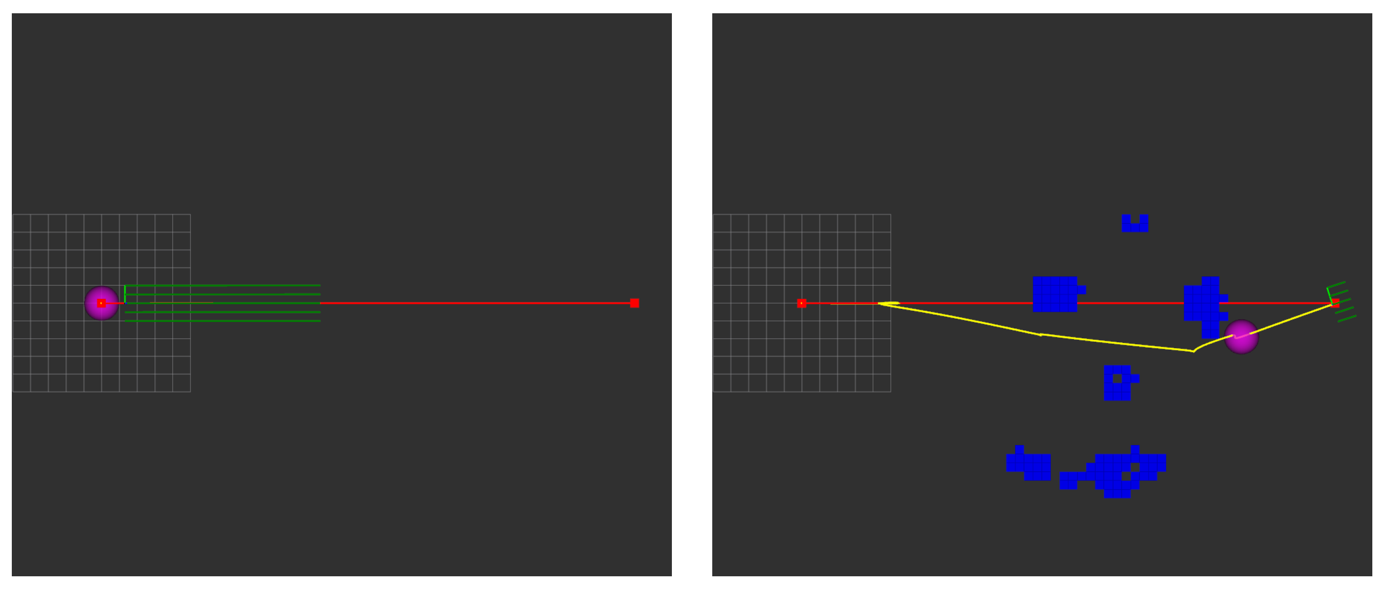
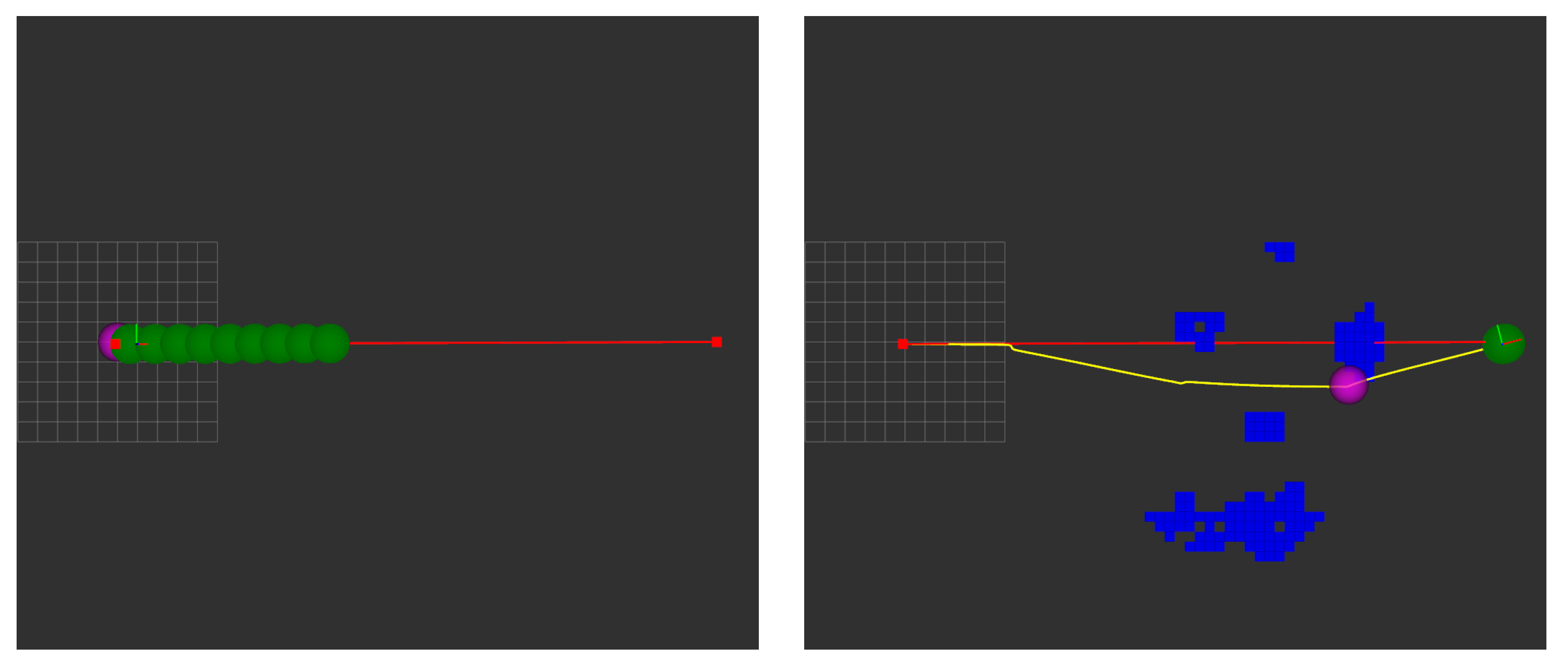
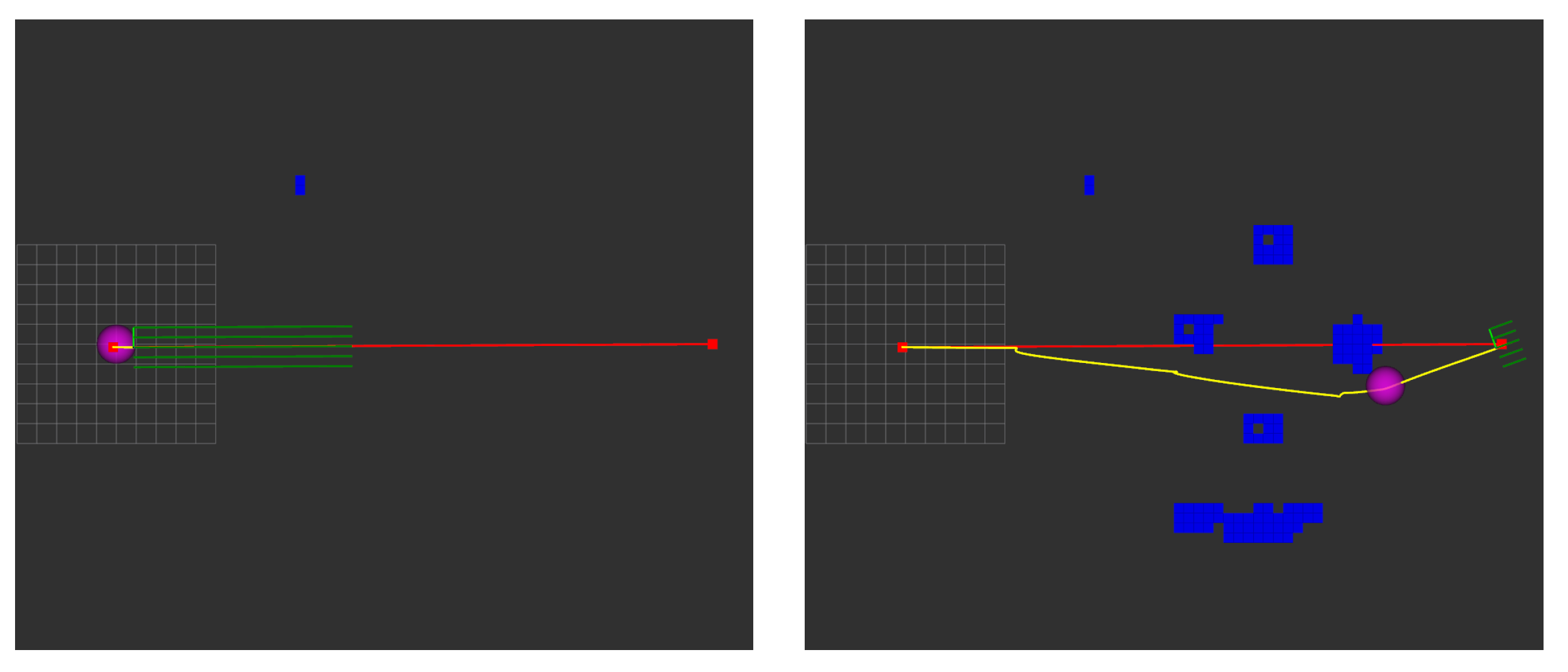
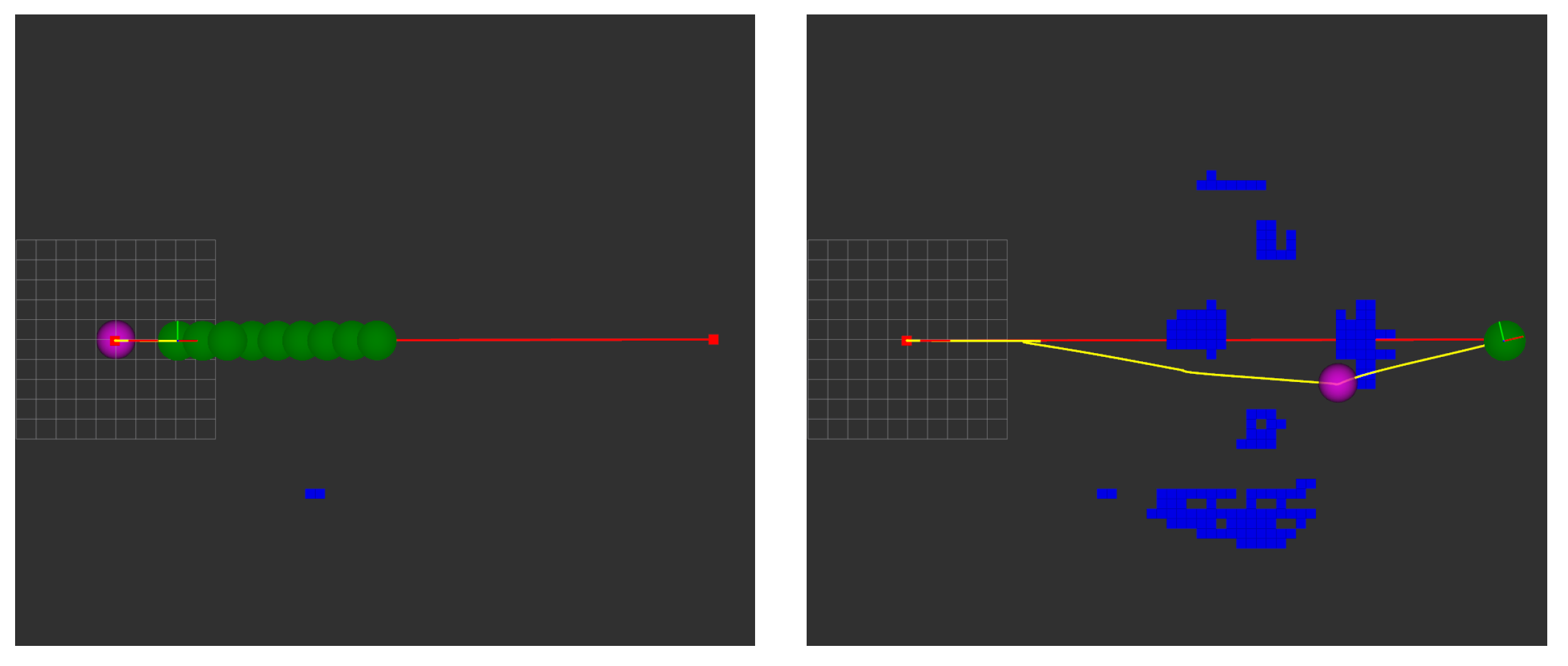
The success of the algorithm was tested using both approaches. Figure 14 and Figure 15 (CPU and GPU, respectively) show the trajectories chosen to avoid collisions with the tower cranes. It can be observed that the algorithm is successful in both cases, generating similar, but not equal, avoidance paths (in yellow).
Processing Times
The processing times presented result from two trials with the same set of waypoints. However, they are not from the exact same flight test, and some quantities may vary, like the number of environment voxels, due to the probabilistic nature of the map representation and UAV pose.
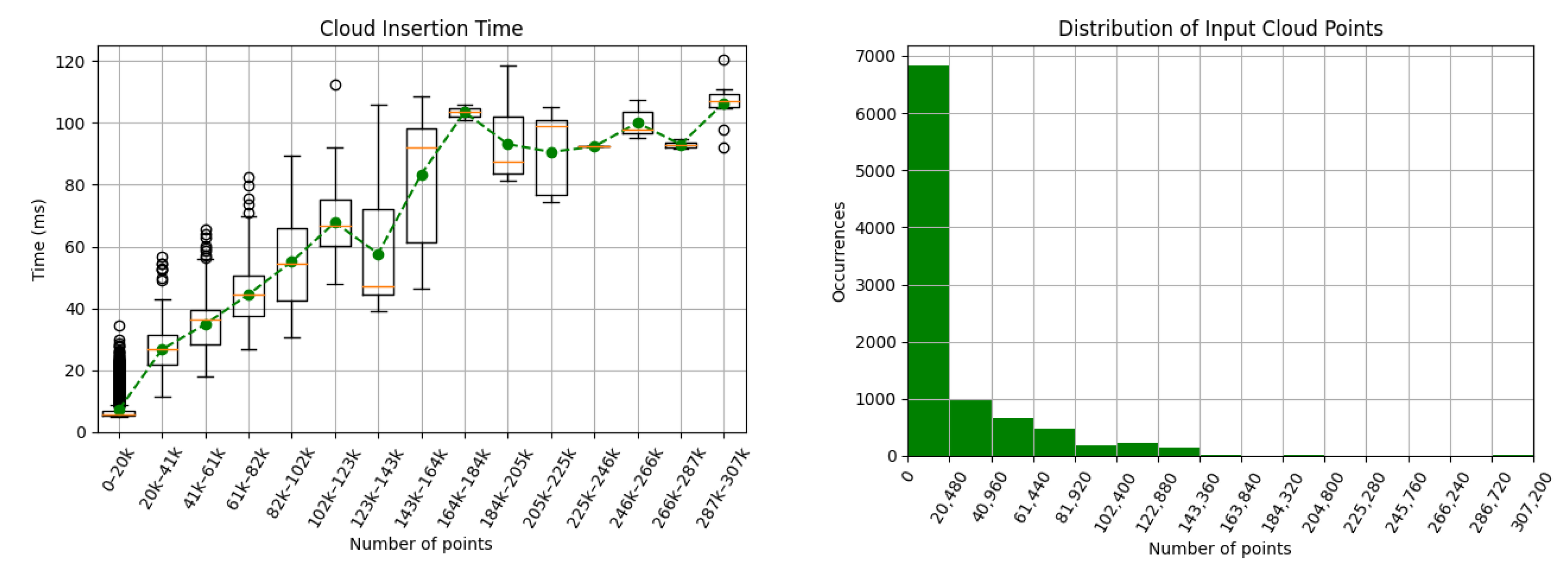
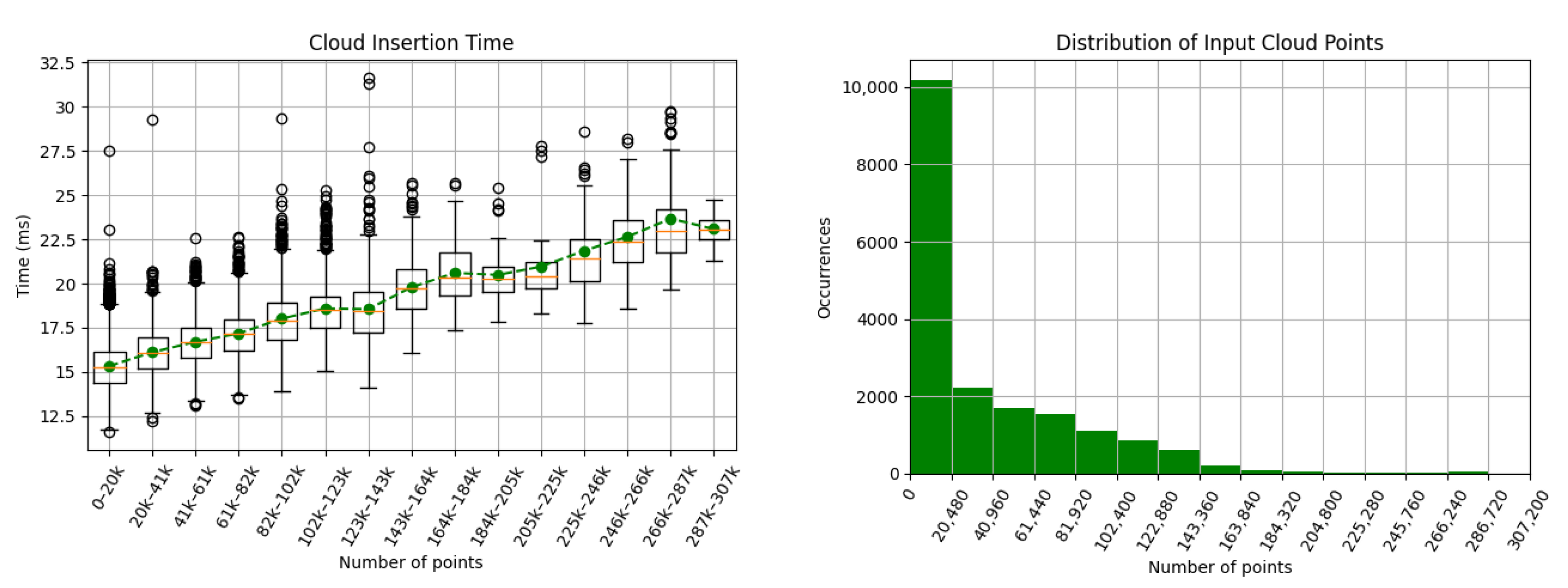
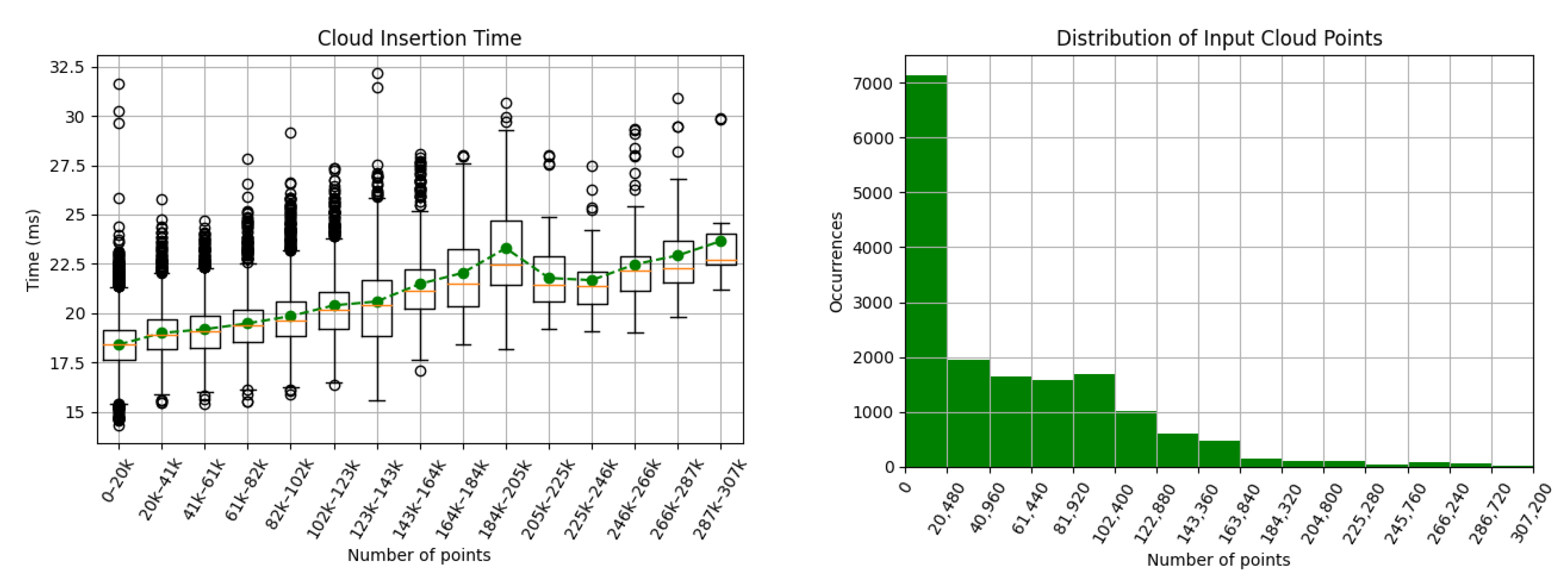
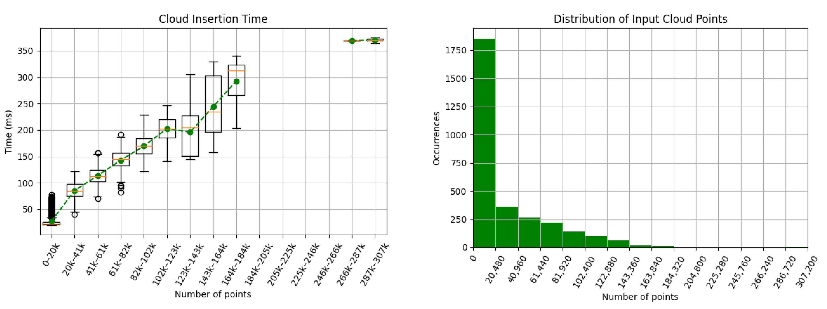
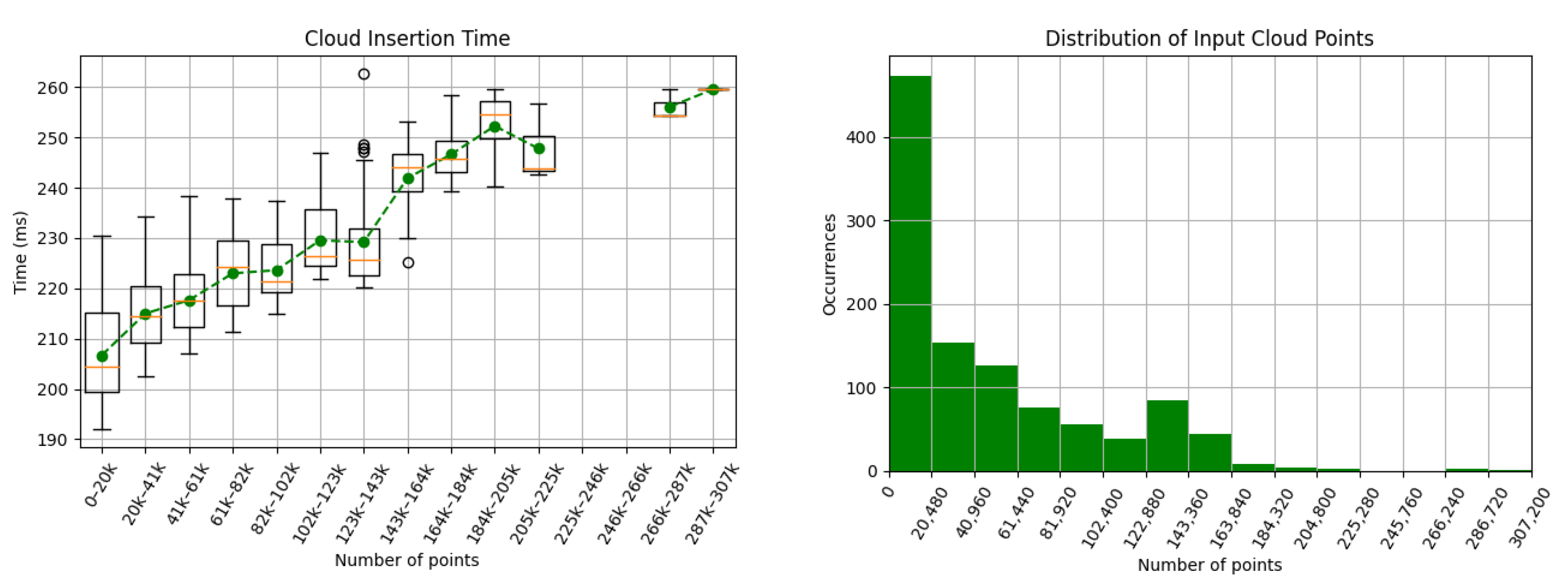
Point Cloud Insertion: Figure 16 and Figure 17 show the times of inserting the point cloud into the map representation for the CPU and GPU approaches. The CPU approach shows a clear linear dependence of the insertion times with the increase in input points. The GPU approach also shows a linear but much smaller dependence on the number of inserted occupied points.
Since the GPU insertion times are low and less dependent on the number of input points, on another trial, the free points were also added to the map in the directions that no data are provided, using a range of 10 m from the camera. This makes the number of input points constant (307,200 points). Figure 18 shows the new insertion times as a function of the number of occupied points. Comparing this to Figure 17, there is not much of an effect, as the linear dependence is only due to additional checking of the occupied points. This also shows that the insertion times are mainly due to CPU data treatment before insertion and CPU-GPU data streams communication overhead. The implementation of this feature increases the map quality, since it erodes outliers.
It is worth noting that the CPU approach tends to have faster insertion times for depth clouds below 20 thousand points, which has occurred in most of the flight.
Obstacle Detection The search for threatening obstacles relies on the cylinder approximation methods described in Section 4.1.2 and Section 4.2.2.
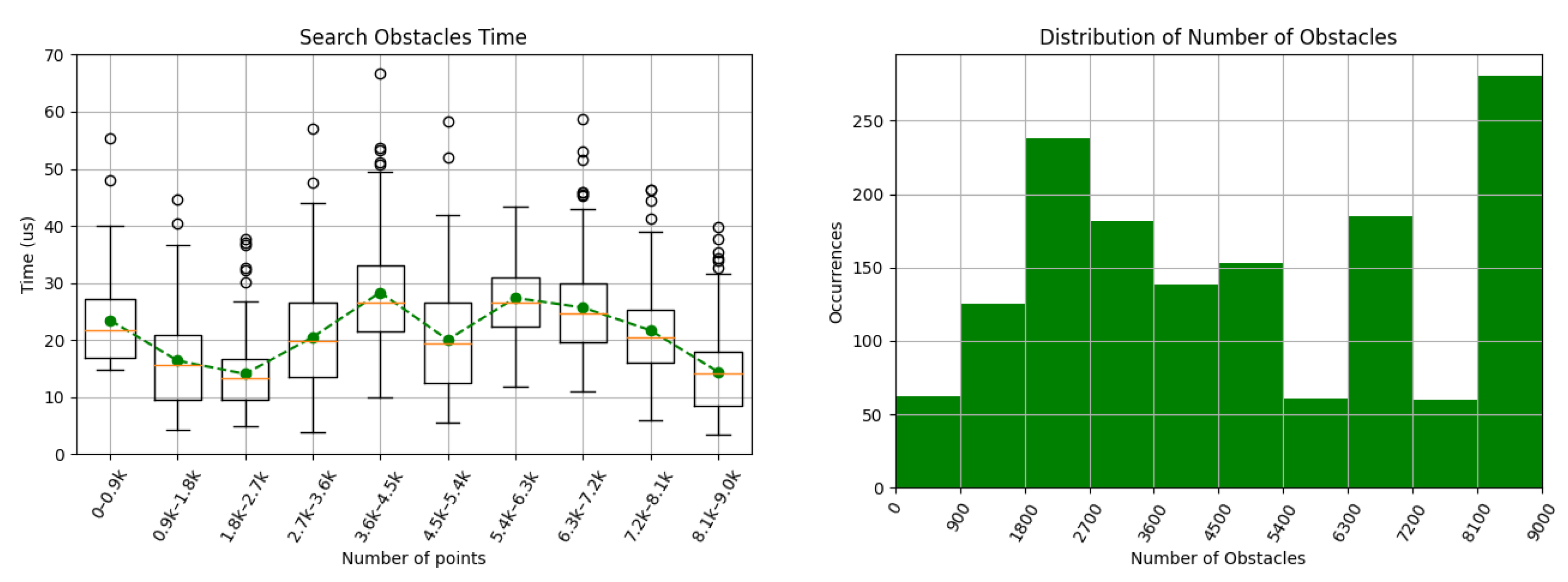
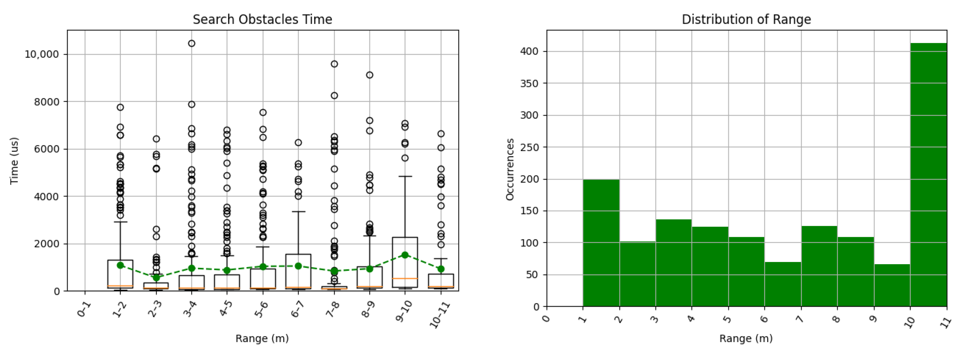
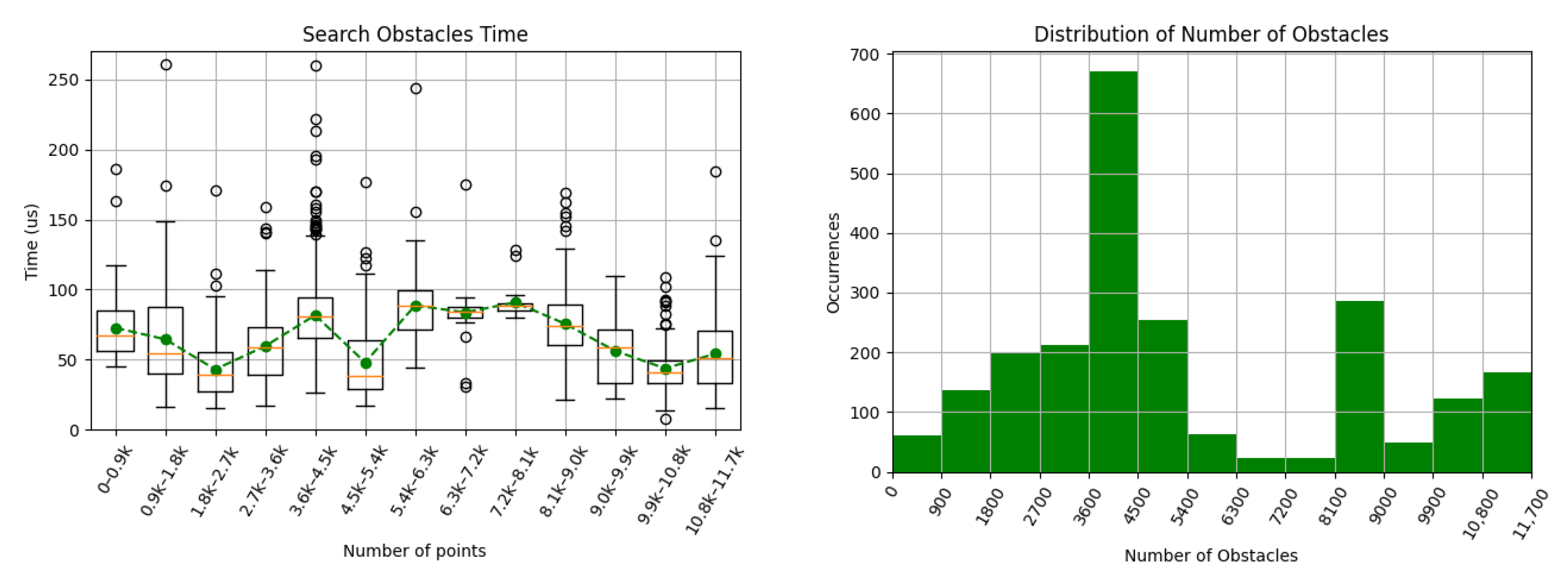
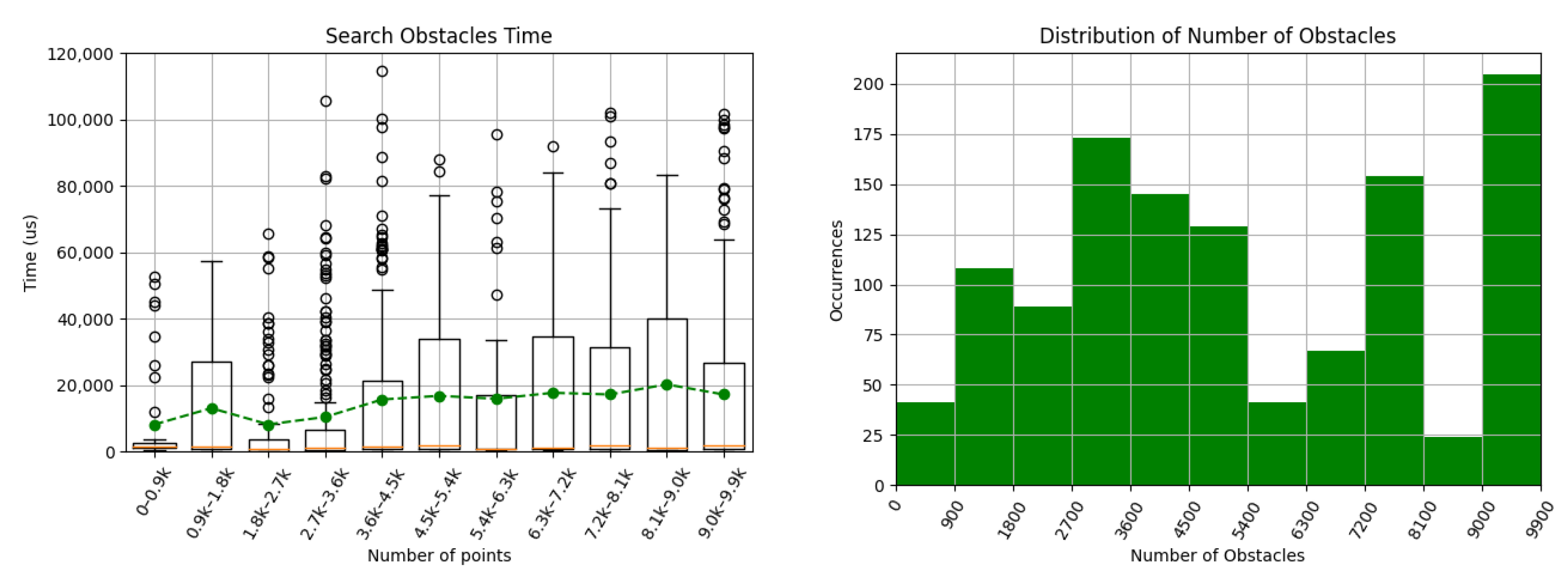
Figure 19 and Figure 20 depict the times used to verify the need to compute an avoidance path, given the number of occupied voxels in the environment map representation. No clear dependence on the number of occupied nodes is shown in the graphs, being the variations mainly due to the CPU load fluctuations since it was also running the simulation environment.
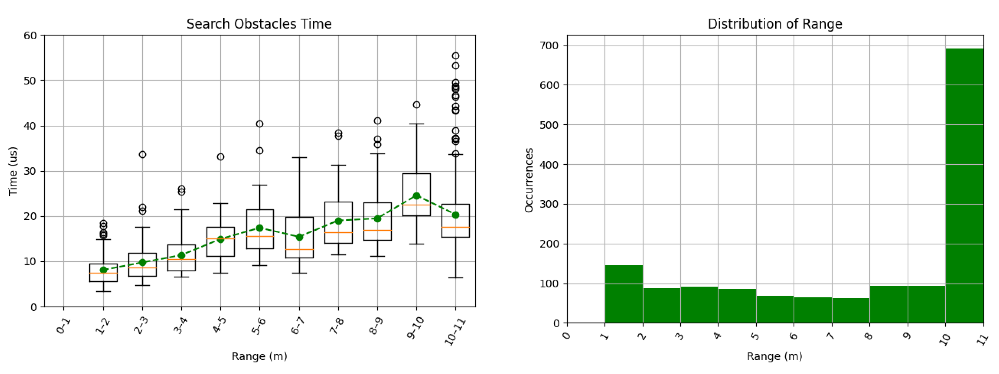
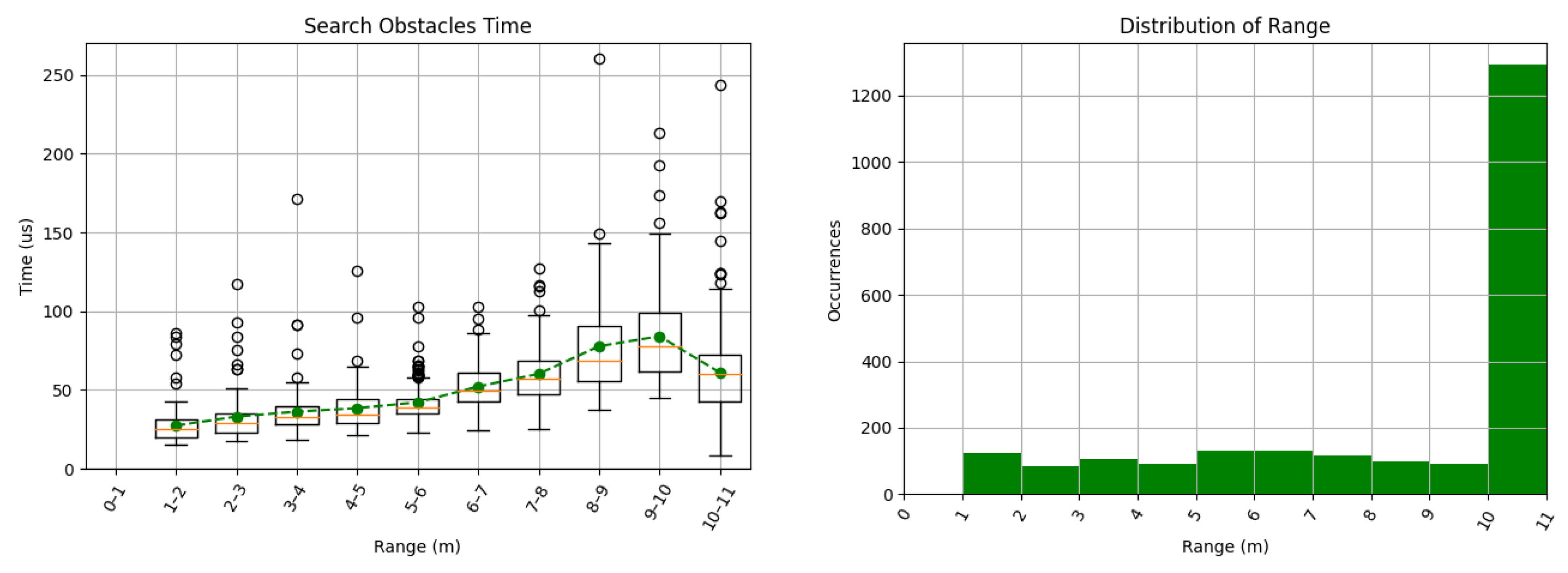
The same analysis was performed for the dependence on the search range L (Figure 21 and Figure 22). The CPU approach with ray cast shows some dependence on the range, but no dependence is observed for the sphere approach.
Regarding the obstacle search times, the CPU approach had by far the best results, showing that the ray firing strategy is much more efficient than the method with the sphere approximation, despite its dependence on the range.
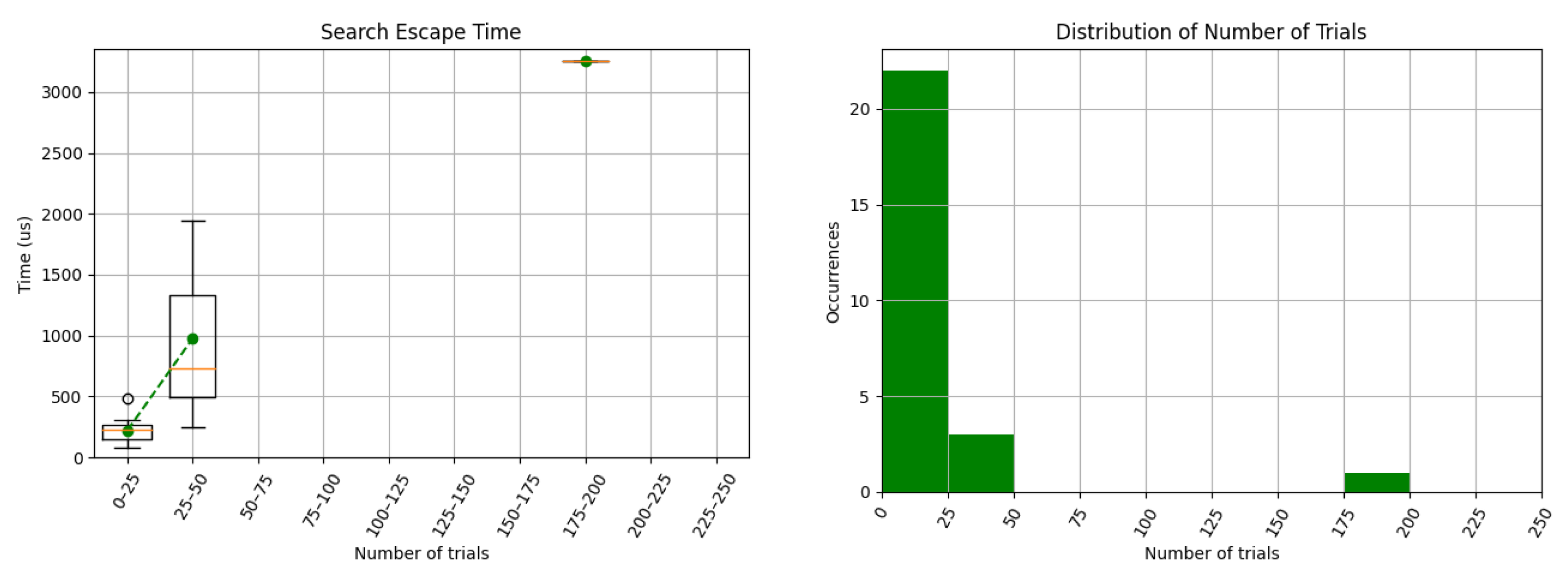
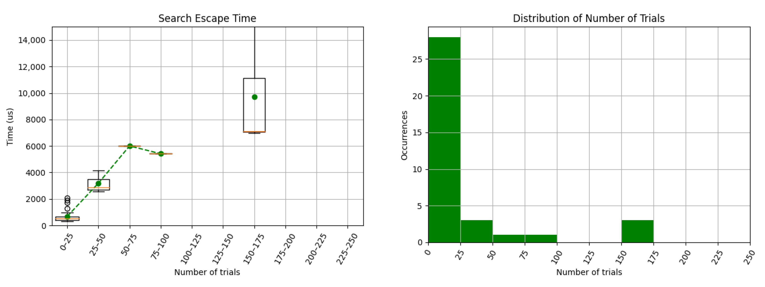
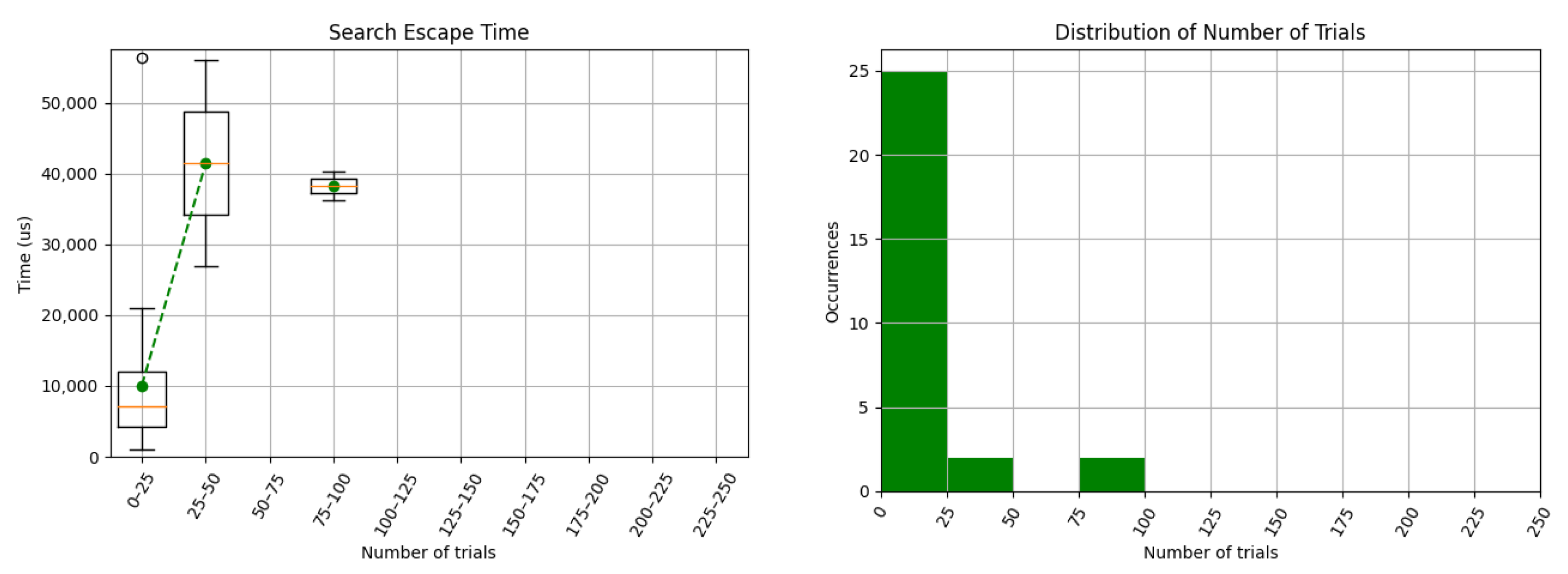
Avoidance Calculation: Finally, the time required to calculate a valid avoidance path was analysed. In this trial, the maximum number of iterations was never reached. Due to the iterative nature of the search and the dependence on the obstacle detection procedures, a linear dependence on calculations times is expected with the number of iterations, which is confirmed in Figure 23 and Figure 24. Additionally, the GPU approach takes more time to find a valid escape point. In Figure 24, the decreasing time for 75–100 iterations might be due to the early cycle break strategy if an obstacle is found near the drone.
5.2.2. Jetson Nano
The evaluation steps in the Jetson Nano were the same as in the laptop; however, in this case, the laptop is responsible for running the simulation environment, while the Jetson Nano is fully dedicated to run the developed algorithm, connected via LAN to the laptop. This configuration removes the heavy simulation from the Jetson core, but relies on the LAN speed.
Success
Processing Times
The set of waypoints is the same used in the laptop evaluation.
Point Cloud Insertion: The times for inserting the point clouds are depicted in Figure 27 and Figure 28 for CPU and GPU. Both approaches have a dependence on the point cloud size, being more notorious for the CPU. The results presented in Figure 28 include the insertion of free points, used to clear outliers that might exist in the map from previous insertions.
On Jetson Nano, the GPU implementation is only advantageous for depth clouds above nearly 150 thousand points, which rarely happened during the flight. This suggests that there exists a bottleneck in the CPU-GPU communication, causing the growth of the insertion times. Using a low-power CPU also affects the performance, since the pre-insertion processing tends to be slower.
In both cases, the large times (compared to the laptop’s evaluation) led to the drop of some depth cloud messages, as can be confirmed by comparing the histograms of occurrences (Figure 16 and Figure 18 for laptop).
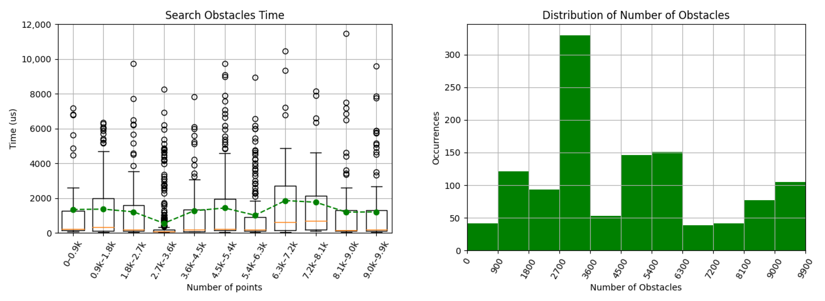
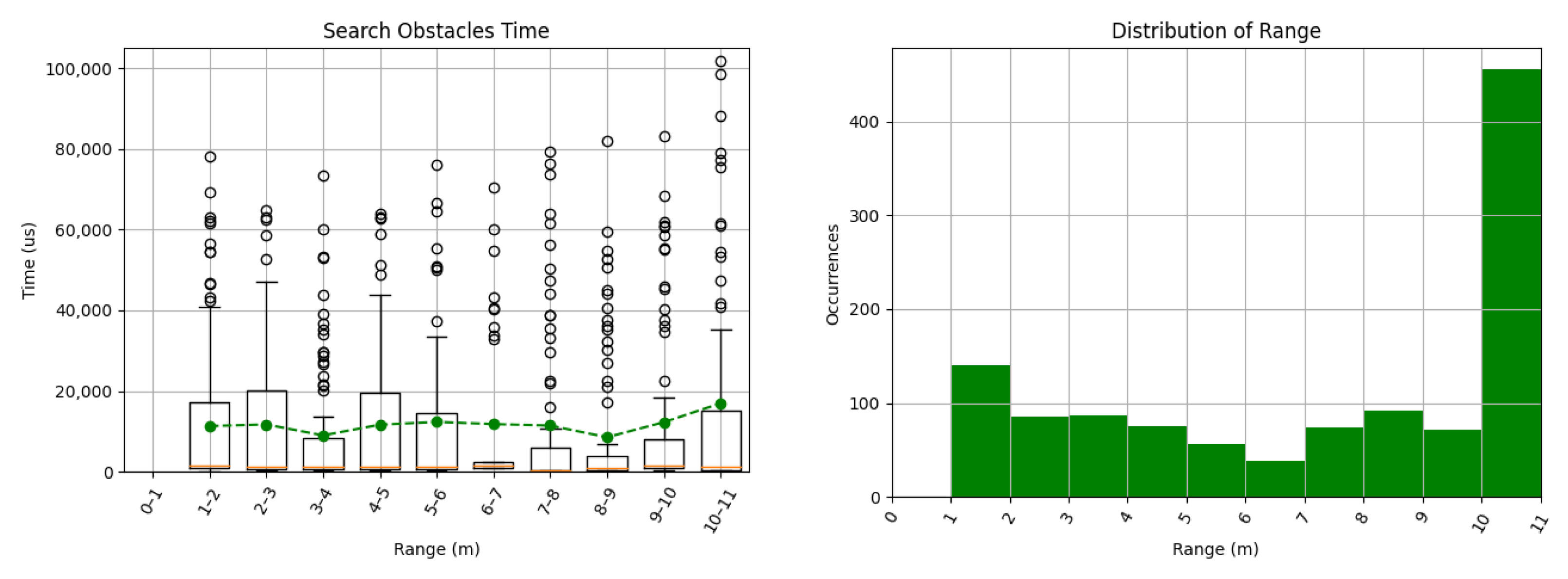
Obstacle Detection: Using the respective approaches for cylinder approximation, described in Section 4.1.2 and Section 4.2.2, the algorithm had the processing times depicted in Figure 29 and Figure 30. None of the cases shows a clear time dependence on the number of obstacles, but the processing time differences (between CPU and GPU) are even more notorious here. For the ray cast method, Jetson Nano is nearly 2 to 3 times slower than the laptop. However, in the case of sphere approximation, the processing time increases 10 times.
Regarding the dependence on the search range L (Figure 31 and Figure 32). Similarly to the laptop evaluation, the CPU approach with ray cast shows some dependence on the range, while no dependence is observed for the sphere approach. The processing time increase, when compared to the laptop approach, is the same as for the number of obstacles analysis, 2–3 times for CPU and 10 times for GPU. This large increase in the GPU approach also suggests the CPU-GPU communication bottleneck, since the sphere method makes requests to the GPU-Voxels distance map.
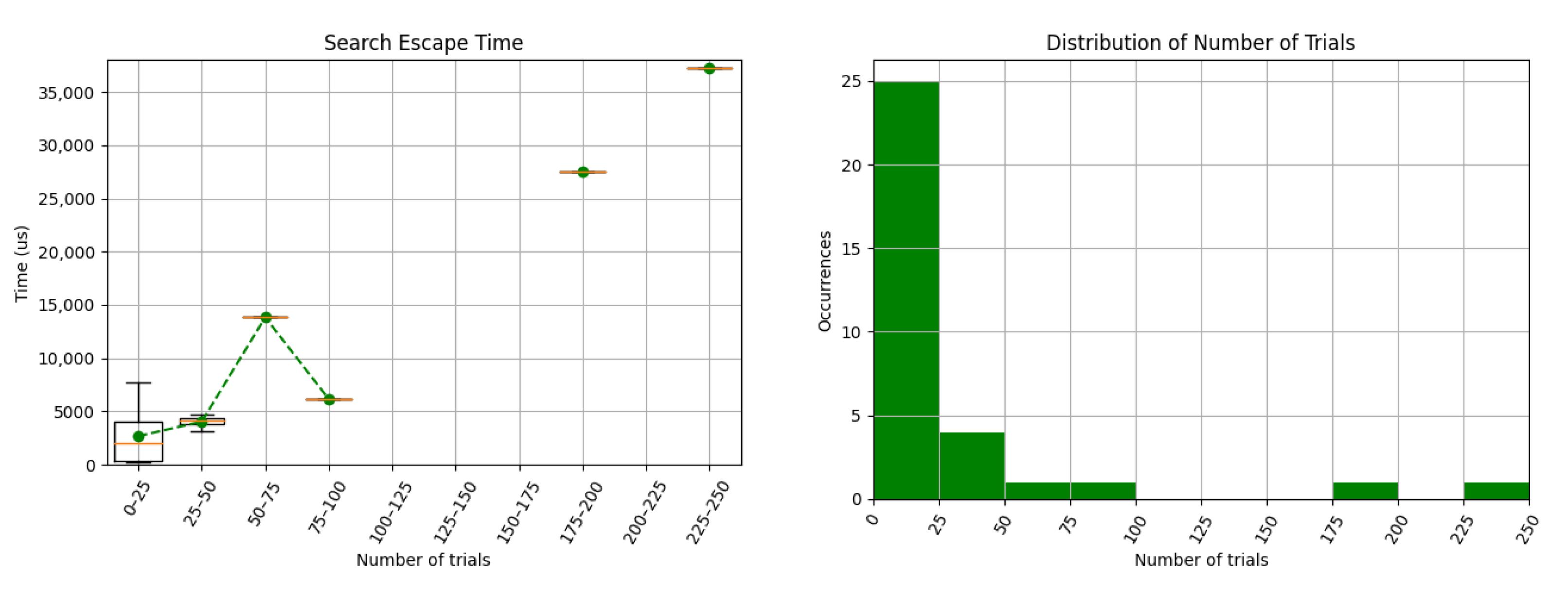
Avoidance Calculation: During the experimental flight, the maximum number of iterations was never reached, and the processing times are presented in Figure 33 and Figure 34. Due to the dependency on the obstacle search strategy, the GPU method requires more time for the same number of iterations; however, the relation between CPU and GPU methods is not constant over the iterations, which again could be due to the early cycle interruption when an obstacle is near the UAV. This situation tends to occur more often with slower processing. Since the vehicle will take longer to perceive the obstacles and stop, the obstacles will be nearer when calculating the avoidance path.
5.3. Second Stage Results
After a complete evaluation of the algorithm in the simulated scenario, the next step was to carry out a preliminary test with the real hardware in a real scenario. For safety reasons, for this first test, the algorithm had no control over the drone navigation, being the safety pilot the responsible for positioning the drone for the sensor acquisition of the environment.
Unlike the offline test, the onboard computer Jetson Nano was now running all the control algorithms, acquiring sensors, logging data to an external disk, and communicating with a ground control station (GCS).
5.3.1. Processing Times
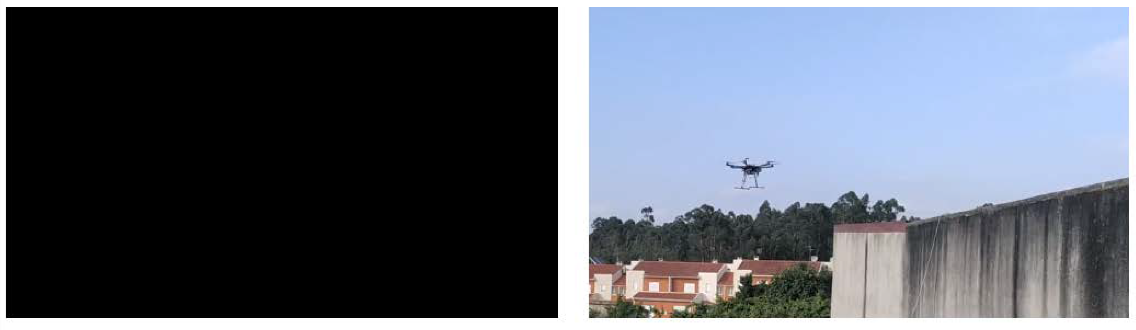
The test setup was simple and consisted only of flying the drone facing a wall (Figure 35) to evaluate the algorithm’s perception and outputs. Both CPU and GPU-based implementations were tested using the same strategy.
Point Cloud Insertion
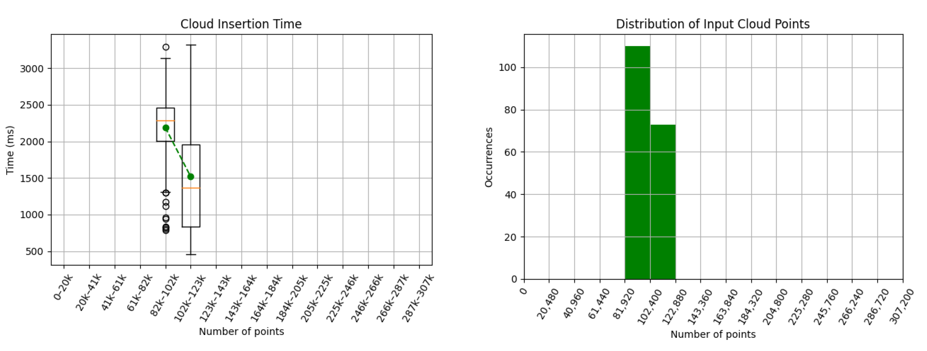
Figure 36 and Figure 37 show the times obtained for inserting the depth cloud in the map representations. The approach using CPU has shown to be entirely not viable to apply in the real scenario. The insertion times of a single medium-size point cloud can take 3 s, not being suitable for the avoidance strategy. This effect occurred due to the high computational load in the CPU, since it was managing other tasks in parallel (like acquiring the camera).
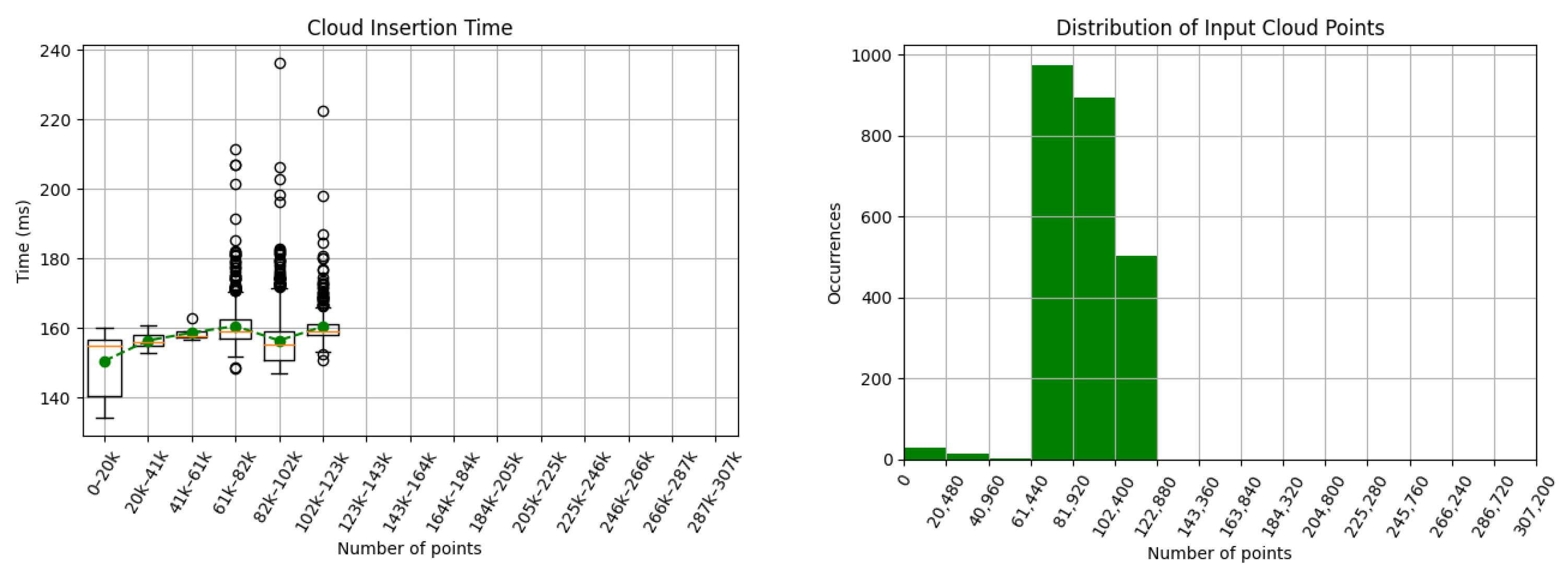
On the other hand, the GPU insertion times were on pair (and even lower) with the results obtained in simulation (see Figure 28). The lower times are due to a difference between the simulated and real Intel Realsense cameras. The simulated camera is configured to send a dense point cloud with the pixels with no value as , allowing to easily implement the strategy of cleaning the environment map by inserting free points. The real camera only sends a stream with points containing valid measures, not being possible to enable the free point insertion methodology. The implementation could be adapted by identifying the pixels that were not received through trigonometric calculations; however, they are computationally expensive and were not implemented for the first trials.
Obstacle Detection and Avoidance Calculation
These operations are mainly CPU-based and, since there was only one waypoint, they have few measurements to plot in a graph. The few values obtained followed the trend of the results presented in the Jetson Nano fully-dedicated operation (Section Processing Times). The obstacle search times using the ray cast in the CPU approach were below s, showing that the point cloud insertion increased time is due to scheduling priorities, since fast tasks keep their processing times.
In both methods, when navigating against the wall, an avoidance procedure was triggered, showing that the obstacles were detected as threats.
6. Discussion
In the results section, some implementation specificities and conditions that led to them have already been discussed. The evaluation had its focus on the processing times of each module on different platforms.
When using the laptop to process the algorithm, the CPU approach is able to correctly insert the depth cloud at a rate of 10–100 Hz, depending on the cloud size, while the GPU is less dependent on the cloud size and can process the data at nearly 50 Hz. Searching for potential obstacles in the map can be done at more than 30 kHz using the ray cast CPU method, but only at 500 Hz when using the sphere with the GPU distance map method. The times for calculating an avoidance trajectory depend strongly on the parameters used (arc length, number of steps, spiral winding) but can be done, in a general map, in less than 1 ms with Octomaps, or 5 ms with the GPU version.
In the fully-dedicated Jetson Nano results, the insertion of point clouds in Octomaps drops to a rate of 2.5–40 Hz, and in GPU-Voxels to an average of 4 Hz. The obstacle detection can be done with a rate of 10 kHz in CPU, while the GPU method only reaches 50 Hz and has some processing time peaks. Dependent on these last values, the avoidance path can be typically found in around 4 ms using ray cast to search possible paths and 50 ms using the cylinder approximation by spheres.
The test in a real scenario has shown the impossibility of using the CPU approach for point cloud insertion due to the heavy CPU load (only reaches 0.4 Hz), but the GPU-Voxels keeps the performance obtained in simulation, with an insertion rate of 6 Hz. The remaining modules had the same performance as in the simulation trials.
From the real scenario results, the straightforward approach would be to implement the GPU-Voxels approach to deal with the CPU load in operation. However, the ray cast feature of Octomaps can greatly reduce the search and avoidance calculation times, being very useful for having a quicker perception and response. Therefore, adding this feature to the GPU approach would make it a good solution for applying in Jetson Nano, not compromising the remaining UAV software modules.
Despite implemented, the strategy of moving to the previous waypoint to recover from local traps was never triggered, since the iterations’ limit when searching for an escape point was never reached. Adding to this, this method needs some extra benchmark in terms of success and quality of the path generated. Being a reactive solution for preventing collisions, the path followed might not be optimal (or even near it). However, the spiral strategy tries to minimise it by deviating from the straight line only when needed, and the distance strictly needed to ensure the safety of the vehicle and structures.
7. Conclusions
In this work, a reactive approach to the collision avoidance problem was developed. Unlike other existing works in the literature, this paper also covers the problem of transforming the data from the perception sensors in the map representation, considering it part of the collision avoidance problem, since the avoidance success highly depends on an accurate map representation.
Two approaches were developed to evaluate both CPU and GPU advantages and limitations. The map representation is based on octrees, and the obstacle’s search relies on a safety volume from the drone, pointing in the direction of the movement. The safety volume is cylindrical, but approximated either by a set of ray firings (CPU approach) or a set of spheres (GPU approach). If the safety volume is crossed, an avoidance procedure is triggered. The avoidance path calculation evaluates a set of candidate escape points that are generated from a spiral-shaped iterative method, centred on the closest threatening object. The escape point (and, therefore, the path) is valid if the safety volume is ensured from the drone to it and from it to the final goal point along a specified distance.
The method was implemented in ROS and validated with Gazebo simulation. It successfully made the UAV navigate in a complex environment, keeping low processing times both in a high-performance laptop and in Jetson Nano, a low-power GPU-enabled computer. The map representation in the CPU used Octomaps, and GPU-Voxels for the GPU implementation. The algorithm was able to deal with point cloud insertion rates of 10–100 Hz using Octomaps in the laptop and 2.5–40 Hz in the Jetson Nano. GPU-Voxels representation had less dependency on the point cloud size, updating the map at 50 Hz in the laptop and 4 Hz in the low-power computer. The ray cast method to approximate the cylindrical safety volume has provided a tool to search obstacles at 10 kHz in the Jetson Nano.
Due to the high CPU load caused by the other components running, the Octomaps performed poorly in a real scenario for updating the map, but GPU-Voxels kept the performance obtained in simulation. Generally, the GPU map representation provided a solution almost independent of the point cloud size, while the CPU ray cast approach was the best for searching potential obstacles.
It is worth noting that the GPU-Voxels native implementation is for Intel-based CPU architectures, while Jetson Nano has an ARM-based CPU.
Future Work
In order to improve the developed work so far, an implementation of ray cast in GPU seems to be a promising path to follow, accompanied by a deeper study of GPU-Voxels structure and implementation. An alternative to this framework is the Nvidia GVDB-Voxels [35]. Other map representations not based on octrees shall also be considered.
The implementation code can be further optimised, avoiding floating-point operations and replacing trigonometric functions with lookup tables. In pair with this, a focus on the UAV control can also help to improve the performance. If the direction change between waypoints is not significant, the drone could keep moving while rotating, having smoother behaviours.
For improving the robustness and efficiency of the algorithm, further real-scenario tests are envisioned to deal with the real-world variables and uncertainties that are often not present in the simulation environments. The testing of the algorithm in a Jetson Nvidia Xavier NX [36] is also planned to evaluate whether it is sufficient to alleviate the high CPU load suffered by Jetson Nano.
Author Contributions
Conceptualisation, F.A.; methodology, F.A.; software, F.A. and A.F.; validation, F.A., A.F., T.F. and M.M.; formal analysis, F.A.; investigation, F.A.; resources, L.C.; data curation, F.A.; writing—original draft preparation, F.A. and J.S.C.; writing—review and editing, F.A., J.S.C., A.F., T.F., M.M. and L.C.; visualisation, F.A.; supervision, J.S.C.; project administration, L.C.; funding acquisition, L.C. All authors have read and agreed to the published version of the manuscript.
Funding
This project has received funding from the ECSEL Joint Undertaking (JU) under grant agreement No 783221. This project has also received funding from the ECSEL JU under grant agreement No 783119. The JU receives support from the European Union’s Horizon 2020 research and innovation programme and Austria, Belgium, Czech Republic, Finland, Germany, Greece, Italy, Latvia, Norway, Poland, Portugal, Spain, Sweden.
Institutional Review Board Statement
Not applicable.
Informed Consent Statement
Not applicable.
Data Availability Statement
The data presented in this study are available in the article.
Acknowledgments
The authors would like to thank Beyond Vision Research and Development Group and PDMFC Research and Development Team.
Conflicts of Interest
The authors declare no conflict of interest.
Abbreviations
The following abbreviations are used in this manuscript:
| CPU | Central Processing Unit |
| EVG | Essential Visibility Graphs |
| FOV | Field-Of-View |
| GCS | Ground Control Station |
| GNSS | Global Navigation Satellite System |
| GPU | Graphics Processing Unit |
| LAN | Local Area Network |
| LiDAR | Light Detection And Ranging |
| ORCA | Optimal Reciprocal Collision Avoidance |
| P2P | Peer-to-Peer |
| ROS | Robot Operating System |
| RTK | Real Time Kinematics |
| UAV | Unmanned Aerial Vehicle |
References
- Liew, C.F.; DeLatte, D.; Takeishi, N.; Yairi, T. Recent Developments in Aerial Robotics: A Survey and Prototypes Overview. arXiv 2017, arXiv:1711.10085. [Google Scholar]
- Azevedo, F.; Dias, A.; Almeida, J.; Oliveira, A.; Ferreira, A.; Santos, T.; Martins, A.; Silva, E. LiDAR-Based Real-Time Detection and Modeling of Power Lines for Unmanned Aerial Vehicles. Sensors 2019, 19, 1812. [Google Scholar] [CrossRef] [PubMed] [Green Version]
- Pedro, D.; Mora, A.; Carvalho, J.; Azevedo, F.; Fonseca, J. ColANet: A UAV Collision Avoidance Dataset; Technological Innovation for Life Improvement; Camarinha-Matos, L.M., Farhadi, N., Lopes, F., Pereira, H., Eds.; Springer International Publishing: Cham, Switzerland, 2020; pp. 53–62. [Google Scholar]
- Vergouw, B.; Nagel, H.; Bondt, G.; Custers, B. Drone Technology: Types, Payloads, Applications, Frequency Spectrum Issues and Future Developments. In The Future of Drone Use: Opportunities and Threats from Ethical and Legal Perspectives; Custers, B., Ed.; T.M.C. Asser Press: The Hague, The Netherlands, 2016; pp. 21–45. [Google Scholar] [CrossRef]
- Azevedo, F.; Oliveira, A.; Dias, A.; Almeida, J.; Moreira, M.; Santos, T.; Ferreira, A.; Martins, A.; Silva, E. Collision avoidance for safe structure inspection with multirotor UAV. In Proceedings of the 2017 European Conference on Mobile Robots (ECMR), Paris, France, 6–8 September 2017; pp. 1–7. [Google Scholar] [CrossRef] [Green Version]
- Kavraki, L.E.; Svestka, P.; Latombe, J.; Overmars, M.H. Probabilistic roadmaps for path planning in high-dimensional configuration spaces. IEEE Trans. Robot. Autom. 1996, 12, 566–580. [Google Scholar] [CrossRef] [Green Version]
- Lavalle, S.M. Rapidly-Exploring Random Trees: A New Tool for Path Planning; Technical Report TR 98-11; Computer Science Department, Iowa State University: Ames, IA, USA, 1998. [Google Scholar]
- Huang, S.; Teo, R.S.H.; Tan, K.K. Collision avoidance of multi unmanned aerial vehicles: A review. Annu. Rev. Control 2019, 48, 147–164. [Google Scholar] [CrossRef]
- Hornung, A.; Wurm, K.M.; Bennewitz, M.; Stachniss, C.; Burgard, W. OctoMap: An efficient probabilistic 3D mapping framework based on octrees. Auton. Robot. 2013, 34, 189–206. [Google Scholar] [CrossRef] [Green Version]
- Maier, D.; Hornung, A.; Bennewitz, M. Real-time navigation in 3D environments based on depth camera data. In Proceedings of the 2012 12th IEEE-RAS International Conference on Humanoid Robots (Humanoids 2012), Osaka, Japan, 29 November–1 December 2012; pp. 692–697. [Google Scholar] [CrossRef]
- Chestnutt, J.; Takaoka, Y.; Suga, K.; Nishiwaki, K.; Kuffner, J.; Kagami, S. Biped navigation in rough environments using on-board sensing. In Proceedings of the 2009 IEEE/RSJ International Conference on Intelligent Robots and Systems, St. Louis, MO, USA, 10–15 October 2009; pp. 3543–3548. [Google Scholar] [CrossRef] [Green Version]
- Gutmann, J.S.; Fukuchi, M.; Fujita, M. 3D Perception and Environment Map Generation for Humanoid Robot Navigation. Int. J. Robot. Res. 2008, 27, 1117–1134. [Google Scholar] [CrossRef]
- Nieuwenhuisen, M.; Behnke, S. Hierarchical Planning with 3D Local Multiresolution Obstacle Avoidance for Micro Aerial Vehicles. In Proceedings of the ISR/Robotik 2014, 41st International Symposium on Robotics, Munich, Germany, 2–3 June 2014; pp. 1–7. [Google Scholar]
- Grzonka, S.; Grisetti, G.; Burgard, W. A Fully Autonomous Indoor Quadrotor. IEEE Trans. Robot. 2012, 28, 90–100. [Google Scholar] [CrossRef] [Green Version]
- Hart, P.E.; Nilsson, N.J.; Raphael, B. A Formal Basis for the Heuristic Determination of Minimum Cost Paths. IEEE Trans. Syst. Sci. Cybern. 1968, 4, 100–107. [Google Scholar] [CrossRef]
- Koenig, S.; Likhachev, M. Fast replanning for navigation in unknown terrain. IEEE Trans. Robot. 2005, 21, 354–363. [Google Scholar] [CrossRef]
- Hrabar, S. An evaluation of stereo and laser-based range sensing for rotorcraft unmanned aerial vehicle obstacle avoidance. J. Field Robot. 2012, 29, 215–239. [Google Scholar] [CrossRef]
- Merz, T.; Kendoul, F. Beyond visual range obstacle avoidance and infrastructure inspection by an autonomous helicopter. In Proceedings of the 2011 IEEE/RSJ International Conference on Intelligent Robots and Systems, San Francisco, CA, USA, 25–30 September 2011; pp. 4953–4960. [Google Scholar] [CrossRef]
- Hrabar, S. Reactive obstacle avoidance for Rotorcraft UAVs. In Proceedings of the 2011 IEEE/RSJ International Conference on Intelligent Robots and Systems, San Francisco, CA, USA, 25–30 September 2011; pp. 4967–4974. [Google Scholar] [CrossRef]
- Vanneste, S.; Bellekens, B.; Weyn, M. 3DVFH+: Real-Time Three-Dimensional Obstacle Avoidance Using an Octomap. In Proceedings of the CEUR Workshop Proceedings, York, UK, 21 July 2014; Volume 1319. [Google Scholar]
- Ulrich, I.; Borenstein, J. VFH+: Reliable obstacle avoidance for fast mobile robots. In Proceedings of the 1998 IEEE International Conference on Robotics and Automation (Cat. No.98CH36146), Leuven, Belgium, 20 May 1998; Volume 2, pp. 1572–1577. [Google Scholar] [CrossRef]
- Alejo, D.; Cobano, J.A.; Heredia, G.; Ollero, A. Optimal Reciprocal Collision Avoidance with mobile and static obstacles for multi-UAV systems. In Proceedings of the 2014 International Conference on Unmanned Aircraft Systems (ICUAS), Orlando, FL, USA, 27–30 May 2014; pp. 1259–1266. [Google Scholar] [CrossRef]
- Blasi, L.; D’Amato, E.; Mattei, M.; Notaro, I. Path Planning and Real-Time Collision Avoidance Based on the Essential Visibility Graph. Appl. Sci. 2020, 10, 5613. [Google Scholar] [CrossRef]
- Du, Y.; Zhang, X.; Nie, Z. A Real-Time Collision Avoidance Strategy in Dynamic Airspace Based on Dynamic Artificial Potential Field Algorithm. IEEE Access 2019, 7, 169469–169479. [Google Scholar] [CrossRef]
- Loquercio, A.; Maqueda, A.I.; del Blanco, C.R.; Scaramuzza, D. DroNet: Learning to Fly by Driving. IEEE Robot. Autom. Lett. 2018, 3, 1088–1095. [Google Scholar] [CrossRef]
- Falanga, D.; Kleber, K.; Scaramuzza, D. Dynamic obstacle avoidance for quadrotors with event cameras. Sci. Robot. 2020, 5, eaaz9712. [Google Scholar] [CrossRef] [PubMed]
- Hermann, A.; Drews, F.; Bauer, J.; Klemm, S.; Roennau, A.; Dillmann, R. Unified GPU voxel collision detection for mobile manipulation planning. In Proceedings of the 2014 IEEE/RSJ International Conference on Intelligent Robots and Systems, Chicago, IL, USA, 14–18 September 2014. [Google Scholar] [CrossRef]
- Quigley, M.; Conley, K.; Gerkey, B.P.; Faust, J.; Foote, T.; Leibs, J.; Wheeler, R.; Ng, A.Y. ROS: An open-source Robot Operating System. In Proceedings of the ICRA Workshop on Open Source Software in Robotics, Kobe, Japan, 12–13 May 2009. [Google Scholar]
- Curran, W.; Thornton, T.; Arvey, B.; Smart, W.D. Evaluating impact in the ROS ecosystem. In Proceedings of the 2015 IEEE International Conference on Robotics and Automation (ICRA), Seattle, WA, USA, 26–30 May 2015; pp. 6213–6219. [Google Scholar] [CrossRef]
- Damm, C. Object Detection in 3D Point Clouds. Ph.D. Thesis, Institut für Informatik der Freien Universität Berlin, Berlin, Germany, 2016. [Google Scholar]
- HEIFU Drone. Available online: https://www.beyond-vision.pt/product/heifu-drone (accessed on 20 April 2021).
- Pixhawk®. Available online: https://pixhawk.org (accessed on 20 April 2021).
- Jetson Nano Developer Kit. Available online: https://developer.nvidia.com/embedded/jetson-nano-devkit (accessed on 21 April 2021).
- Intel® Realsense™ Depth Camera D435i. Available online: https://www.intelrealsense.com/depth-camera-d435i (accessed on 20 April 2021).
- NVIDIA® GVDB Voxels. Available online: https://developer.nvidia.com/gvdb (accessed on 29 April 2021).
- Jetson Xavier NX Developer Kit. Available online: https://developer.nvidia.com/embedded/jetson-xavier-nx-devkit (accessed on 29 April 2021).
Figure 1.
Algorithm representation of [5].
Figure 1.
Algorithm representation of [5].

Figure 2.
Octree hierarchical representation [9]. Occupied voxels in black and free in white. On the right, parent voxels represented as circles and child as squares.
Figure 2.
Octree hierarchical representation [9]. Occupied voxels in black and free in white. On the right, parent voxels represented as circles and child as squares.

Figure 3.
Environment voxelised representation at multiple resolutions [9].
Figure 3.
Environment voxelised representation at multiple resolutions [9].

Figure 4.
Structure of software components in GPU-Voxels [27]. The red area corresponds to CPU components, while the blue area is GPU’s.
Figure 4.
Structure of software components in GPU-Voxels [27]. The red area corresponds to CPU components, while the blue area is GPU’s.

Figure 5.
Properties of the implemented storage structures [27]. Voxel Map in red, Octree in green, and Voxel Lists in blue.
Figure 5.
Properties of the implemented storage structures [27]. Voxel Map in red, Octree in green, and Voxel Lists in blue.

Figure 6.
Collision avoidance high-level pipeline. Blue blocks are related with the point cloud insertion and representation.
Figure 6.
Collision avoidance high-level pipeline. Blue blocks are related with the point cloud insertion and representation.

Figure 7.
Collision avoidance high-level pipeline with 3D representation skip.

Figure 8.
Orthogonal cross section of cylinder approximation.

Figure 9.
Archimedean spiral samples with a constant arc length. Blue points are considered valid for further calculations. Red crosses are candidate escape points rejected beforehand to avoid very low altitude flights.
Figure 9.
Archimedean spiral samples with a constant arc length. Blue points are considered valid for further calculations. Red crosses are candidate escape points rejected beforehand to avoid very low altitude flights.

Figure 10.
Sphere approximation for cylinder approximation [19].
Figure 10.
Sphere approximation for cylinder approximation [19].

Figure 11.
Flowchart of the method.

Figure 12.
HEIFU prototype (left) and Gazebo simulation model (right).

Figure 13.
Simulation scenario for evaluating the algorithm’s success.

Figure 14.
Success test using CPU approach in laptop (top view). UAV path in yellow. Green rays are the safety volume; Red line is the straight-line connection between the starting position and the waypoint. Pink sphere is the last escape point used. Blue cubes represent occupied voxels.
Figure 14.
Success test using CPU approach in laptop (top view). UAV path in yellow. Green rays are the safety volume; Red line is the straight-line connection between the starting position and the waypoint. Pink sphere is the last escape point used. Blue cubes represent occupied voxels.

Figure 15.
Success test using GPU approach in laptop (top view). UAV path in yellow. Green spheres are the safety volume; Red line is the straight-line connection between the starting position and the waypoint. Pink sphere is the last escape point used. Blue cubes represent occupied voxels.
Figure 15.
Success test using GPU approach in laptop (top view). UAV path in yellow. Green spheres are the safety volume; Red line is the straight-line connection between the starting position and the waypoint. Pink sphere is the last escape point used. Blue cubes represent occupied voxels.

Figure 16.
Point cloud insertion times using CPU approach in laptop.

Figure 17.
Point cloud insertion times using GPU approach in laptop.

Figure 18.
Point cloud and free points insertion times using GPU approach in laptop.

Figure 19.
Obstacle search times with respect to the number of occupied voxels using CPU approach
in laptop.
Figure 19.
Obstacle search times with respect to the number of occupied voxels using CPU approach
in laptop.

Figure 20.
Obstacle search times with respect to the number of occupied voxels using GPU approach
in laptop.
Figure 20.
Obstacle search times with respect to the number of occupied voxels using GPU approach
in laptop.

Figure 21.
Obstacle search times with respect to the search range using CPU approach in laptop.

Figure 22.
Obstacle search times with respect to the search range using GPU approach in laptop.

Figure 23.
Avoidance path calculation times using CPU approach in laptop.

Figure 24.
Avoidance path calculation times using GPU approach in laptop.

Figure 25.
Success test using CPU on Jetson Nano (top view). UAV path in yellow. Green rays are
the safety volume; Red line is the straight-line connection between the starting position and the
waypoint. Pink sphere is the last escape point used. Blue cubes represent occupied voxels.
Figure 25.
Success test using CPU on Jetson Nano (top view). UAV path in yellow. Green rays are
the safety volume; Red line is the straight-line connection between the starting position and the
waypoint. Pink sphere is the last escape point used. Blue cubes represent occupied voxels.

Figure 26.
Success test using GPU on Jetson Nano (top view). UAV path in yellow. Green spheres
are the safety volume; Red line is the straight-line connection between the starting position and the
waypoint. Pink sphere is the last escape point used. Blue cubes represent occupied voxels.
Figure 26.
Success test using GPU on Jetson Nano (top view). UAV path in yellow. Green spheres
are the safety volume; Red line is the straight-line connection between the starting position and the
waypoint. Pink sphere is the last escape point used. Blue cubes represent occupied voxels.

Figure 27.
Point cloud insertion times using CPU approach on Jetson Nano.

Figure 28.
Point cloud insertion times using GPU approach on Jetson Nano.

Figure 29.
Obstacle search times with respect to the number of occupied voxels using CPU approach
on Jetson Nano.
Figure 29.
Obstacle search times with respect to the number of occupied voxels using CPU approach
on Jetson Nano.

Figure 30.
Obstacle search times with respect to the number of occupied voxels using GPU approach
on Jetson Nano.
Figure 30.
Obstacle search times with respect to the number of occupied voxels using GPU approach
on Jetson Nano.

Figure 31.
Obstacle search times with respect to the search range using CPU on Jetson Nano.

Figure 32.
Obstacle search times with respect to the search range using GPU on Jetson Nano.

Figure 33.
Avoidance path calculation times using CPU approach on Jetson Nano.

Figure 34.
Avoidance path calculation times using GPU approach on Jetson Nano.

Figure 35.
HEIFU flying in the real test scenario.

Figure 36.
Point cloud insertion times using CPU approach on Jetson Nano in the real scenario.

Figure 37.
Point cloud insertion times using GPU approach on Jetson Nano in the real scenario.

Publisher’s Note: MDPI stays neutral with regard to jurisdictional claims in published maps and institutional affiliations. |
© 2021 by the authors. Licensee MDPI, Basel, Switzerland. This article is an open access article distributed under the terms and conditions of the Creative Commons Attribution (CC BY) license (https://creativecommons.org/licenses/by/4.0/).
Share and Cite
MDPI and ACS Style
Azevedo, F.; Cardoso, J.S.; Ferreira, A.; Fernandes, T.; Moreira, M.; Campos, L. Efficient Reactive Obstacle Avoidance Using Spirals for Escape. Drones 2021, 5, 51. https://0-doi-org.brum.beds.ac.uk/10.3390/drones5020051
AMA Style
Azevedo F, Cardoso JS, Ferreira A, Fernandes T, Moreira M, Campos L. Efficient Reactive Obstacle Avoidance Using Spirals for Escape. Drones. 2021; 5(2):51. https://0-doi-org.brum.beds.ac.uk/10.3390/drones5020051
Chicago/Turabian StyleAzevedo, Fábio, Jaime S. Cardoso, André Ferreira, Tiago Fernandes, Miguel Moreira, and Luís Campos. 2021. "Efficient Reactive Obstacle Avoidance Using Spirals for Escape" Drones 5, no. 2: 51. https://0-doi-org.brum.beds.ac.uk/10.3390/drones5020051