
Fixed-Wing Unmanned Aerial Vehicle 3D-Model-Based Tracking for Autonomous Landing


1
Portuguese Military Research Center (CINAMIL), Portuguese Military Academy (Academia Militar), R. Gomes Freire 203, 1169-203 Lisbon, Portugal
2
Institute for Systems and Robotics (ISR), Instituto Superior Técnico (IST), 1049-001 Lisbon, Portugal
3
Portuguese Navy Research Center (CINAV), Portuguese Naval Academy (Escola Naval), Alfeite, 2800-001 Almada, Portugal
4
NOVA Information Management School (NOVA IMS), Universidade Nova de Lisboa, 1070-312 Lisbon, Portugal
*
Author to whom correspondence should be addressed.
Drones 2023, 7(4), 243; https://0-doi-org.brum.beds.ac.uk/10.3390/drones7040243
Submission received: 8 March 2023
/
Revised: 26 March 2023
/
Accepted: 29 March 2023
/
Published: 30 March 2023
Abstract
:The vast increase in the available computational capability has allowed the application of Particle-Filter (PF)-based approaches for monocular 3D-model-based tracking. These filters depend on the computation of a likelihood function that is usually unavailable and can be approximated using a similarity metric. We can use temporal filtering techniques between filter iterations to achieve better results when dealing with this suboptimal approximation, which is particularly important when dealing with the Unmanned Aerial Vehicle (UAV) model symmetry. The similarity metric evaluation time is another critical concern since we usually want a real-time implementation. We explored, tested, and compared with the same dataset two different types of PFs, (i) an Unscented Bingham Filter (UBiF) and (ii) an Unscented Bingham–Gauss Filter (UBiGaF), using pose optimization in both implementations. Using optimization steps between iterations increases the convergence capability of the filter and decreases the obtained error. A new tree-based similarity metric approach is also explored based on the Distance Transform (DT), allowing a faster evaluation of the possibilities without losing accuracy. The results showed that the obtained pose estimation error is compatible with the automatic landing requirements.
1. Introduction
The Portuguese Exclusive Economic Zone (EEZ) incorporates three large areas associated with the continent (327,667 km), Azores (953,633 km), and Madeira (446,108 km) [1,2]. As a coastal state, Portugal may exercise sovereign rights over managing natural resources and other economic activities (e.g., tidal power) and is also responsible for conserving living resources and fighting against pollution [3].
To assess compliance with the existing regulations and laws, many technologies can be used to perform surveillance, e.g., Synthetic Aperture Radar (SAR) [4], Satellite Automatic Identification System (S-AIS) [5], or Vessel Monitoring System (VMS) [6]. Using SAR images, we can detect non-AIS-transmitting vessels [7]. Nevertheless, the covered area depends on the satellite location, and the detection accuracy depends on the used algorithm [8]. Exploring and using complementary technologies are essential for constant surveillance in the largest area possible.
Currently, Fast Patrol Boats (FPBs) are essential to act on the field and are still extensively used for surveillance in Portuguese territorial waters. Extending the FPB surveillance capability using fixed-wing Unmanned Aerial Vehicles (UAVs) is essential. Still, the small ship dimensions add an extra challenge, mainly in the take-off and landing operations [9,10,11,12,13]. Small-sized fixed-wing UAVs (typically with a payload below 5 kg) can usually be launched by hand [10,14], bringing most of the operational risk to the landing stage. Landing safety is essential to culminate UAV-based missions successfully. There are three major causes of UAV accidents [15]: human, material, and environment (e.g., weather or illumination changes). The vast majority of UAV registered accidents are mainly due to human factors [16,17,18], and investing in the automation of the most-complex maneuvers is essential.
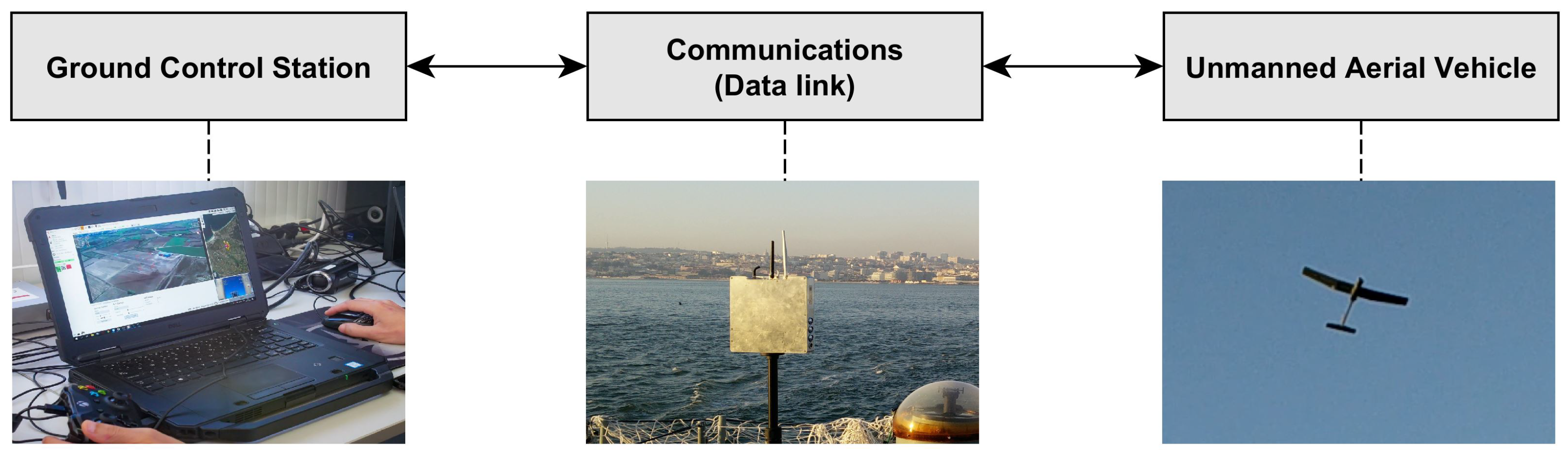
When operating UAVs at sea, we must adapt the system to the existing environment. It is essential to guarantee a waterproof platform, and the communication range and reliability must also be high [19,20]. The UAV system’s basic architecture is composed of a Ground Control Station (GCS), a communications data link, and a vehicle platform [21] (Figure 1).
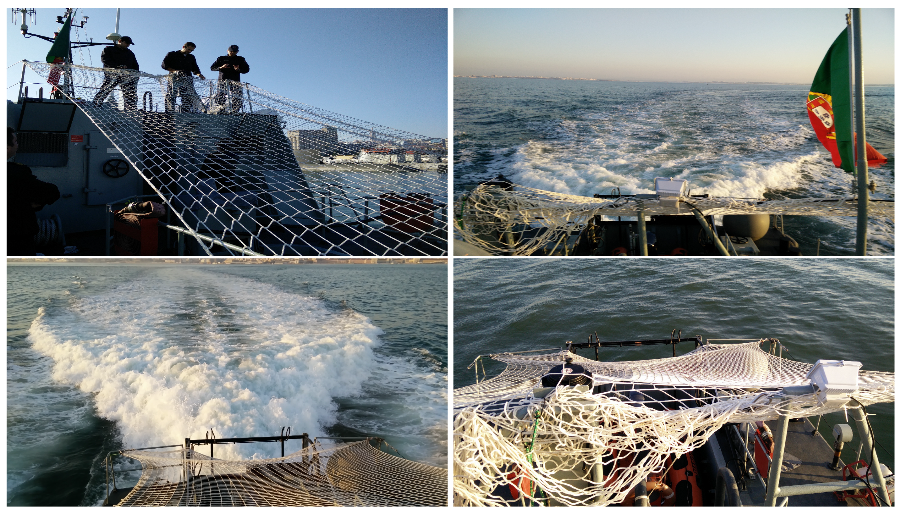
The UAV landing retention system also plays an essential part in the landing operation complexity, and it must be perfectly adapted to the vehicle’s size and weight. A net-based retention system (Figure 2) presents a good compromise between complexity and effectiveness [10,22], being able to be rapidly mounted on any ship without depending on structural changes. If we do not want to capture the UAV directly on the ship, we can also use an external retention system, for instance based on quadcopters [23] using a net [24] or a line [25].
We were trying to land a UAV on a moving platform (ship) in an outdoor environment where we are subject to different meteorological conditions, e.g., illumination, wind, and balance. The UAV is considered a cooperative rigid object with a simple autopilot that maintains a constant trajectory to the landing area. UAVs are also evolving with the development of new structural designs [26], new materials [27], new payloads [28,29], and optimized radar cross-sections [30]. The ship is also considered cooperative and performs maneuvering to adjust the relative speed of the UAV and, consequently, the relative wind. Depending on the ship’s superstructures, we can have wind vortices that can make the UAV adopt an erroneous trajectory.
An automated landing control system can be based on the onboard sensors [21], but we usually do not have enough processing power onboard a small UAV. As an option, we can also rely on the Global Positioning System (GPS), but this system can be affected by jamming or spoofing [31,32,33]. This article used a ground-based monocular Red, Green, and Blue (RGB) vision system with the camera on the ship deck [13,34]. Using a ground-based system, we can access more processing power and implement algorithms to perform the autonomous landing of a UAV with a simple autopilot. Since we used a ground-based Graphics Processing Unit (GPU) system [11,35], which only depend on the GPU processing capabilities, we can easily upgrade it and have access to power without any restrictions. On the other hand, if we use UAV onboard-based algorithms, we need high processing capabilities, which are not easily available in small-sized UAVs. To successfully perform an autonomous landing maneuver, knowing the UAV’s position and its orientation is crucial to predict and control its trajectory. Pose estimation and tracking are widely studied (and still) open problems in Computer Vision (CV), with new methods constantly emerging [36,37].
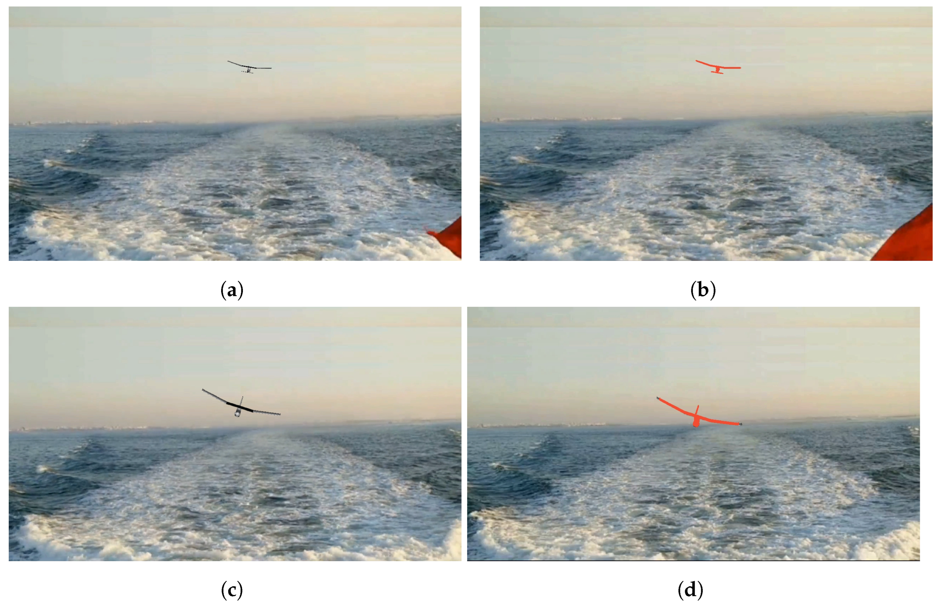
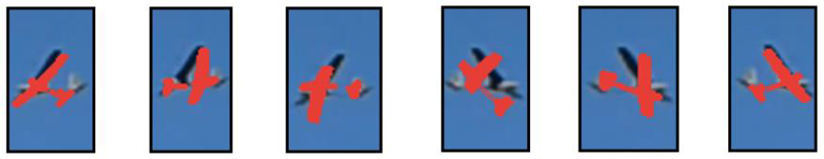
When we know the object we want to detect and have its 3D model or Computer-Aided Design (CAD) model, we can use it to retrieve knowledge from the captured image. We can use Sequential Monte Carlo (SMC) methods or Particle Filter (PF) [38] to establish the 2D/3D correspondence and try to estimate the UAV pose and perform tracking over time [39]. The PFs represents the pose distribution by a set of weighted hypotheses (particles) that explicitly test the object’s projection on the image with a given pose [40]. Despite it being desirable to have a large number of particles to have a fast convergence, particle evaluation is usually very computationally demanding [35], and we need to have a good compromise between speed and accuracy. Some examples of the obtained pose tracking results when using our method can be seen in Figure 3, where the obtained pose estimation is represented in red.
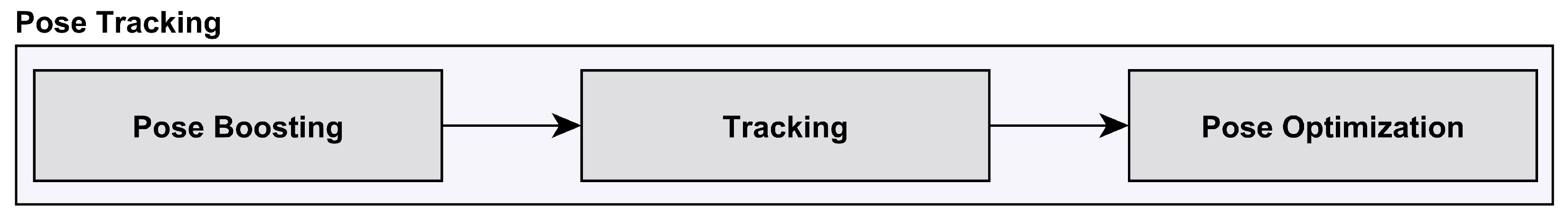
The adopted tracking architecture is divided into: (i) Pose Boosting; (ii) Tracking; (iii) Pose optimization [41,42]. In the Pose Boosting stage, we used Machine Learning (ML) algorithms to detect the UAVs on the captured frame and used a pre-trained database to generate representative pose samples [12,43]. In the Tracking stage, we used a 3D-model-based tracking approach using the UAV CAD model based on a PF approach [42]. In the Pose optimization stage, since we used a sub-optimal similarity metric to approximate the likelihood function iteratively, we included optimization steps to improve the estimate [41].
This article presents the following main developments (innovations): (i) the analysis, test, and comparison on the same dataset of two different PF implementations using pose optimization: (a) an Unscented Bingham Filter (UBiF) [41,42,44] and (b) an Unscented Bingham–Gauss Filter (UBiGaF) [42,45]; (ii) the implementation of a new tree-based similarity metric approach to be able to obtain a faster and more accurate weight estimation; (iii) better analysis and evaluation of how the optimization steps can decrease the filter convergence time; (iv) a validation and comparison between methods using a realistic synthetic dataset. In this article, we did not perform the comparison between UBiF and UBiGaF and more traditional methods such as the Unscented Kalman Filter (UKF) for the orientation estimation since, in [41,42], we already made this comparison and showed that these implementations outperform the UKF. As far as we know, there are no publicly available datasets or other ground-based model-based UAV tracking approaches, making the comparison with other state-of-the-art methods impossible.
The main developments regarding our previous work are: (i) in [42], a tracking architecture using a UBiGaF without pose optimization implementation, which is explored in this article, was proposed; (ii) in [41], we applied optimization steps to the UBiF that is implemented in this article also to the UBiGaF; (iii) in [43], we proposed a distance transform similarity metric that is modified to a tree-based approach to be able to decrease the processing time without a loss in accuracy.
This article is organized as follows. Section 2 presents the related work concerning pose estimation, pose tracking, and UAV tracking. Section 3 details the overall implemented system, detailing the pose boosting, tracking, and optimization stages. In Section 4, we present the experimental results. Finally, in Section 5, we present the conclusions and explore additional ideas for future research work.
2. Related Work
This section describes the related work, namely the pose estimation (Section 2.1), pose tracking (Section 2.2), and UAV tracking methods (Section 2.3).
2.1. Pose Estimation
Pose estimation is a very challenging task, mainly if we are considering only the information coming from a single frame. Some pose estimation methods use Red, Green, Blue, and Depth (RGB-D) cameras to perform data fusion and obtain better estimation results [46,47,48], but those cameras are not usually suitable for outdoor applications. More simplistically, we can use the Efficient Perspective-n-Point (EPnP) algorithm [49] to estimate an object’s pose using a calibrated camera and the correspondence between known 3D object points in the 2D RGB captured frame [50]. We can also compare the captured RGB frame with pre-computed features from the object (template matching), usually obtaining a rough pose estimation [46]. Currently, most applied pose estimation methods are not based on hand-crafted features and algorithms, but rely on deep learning methods using a structure adapted to the application. Sometimes, this structure is poorly optimized, using very deep networks and many parameters without specific design criteria, slowing the training and prediction. Usually, some of the deep learning pose estimation methods start with the detection of a Region Of Interest (ROI) in the frame (object position on the captured frame) [51,52] and then perform pose estimation using additional methods [53,54]. Alternatively, the Deep Neural Networks (DNNs) that perform the detection and pose estimation directly in an encapsulated architecture are increasing and represent the vast majority of the currently existing applications [55,56,57].
2.2. Pose Tracking
The main difference between pose estimation and pose tracking relies on using temporal information to perform the estimation. This temporal information can be only from the last frame or even from other instants in time. Some methods, as described for pose estimation, also use RGB-D cameras to perform data fusion for tracking [58,59,60]. We can use a system designed for single- [61] or multi-object [62] tracking that can perform the tracking of unknown objects (without any a priori information) [63,64] or use the object information (e.g., size or color) [65,66] to develop our tracking algorithms. Currently, most applied pose tracking methods rely on deep learning methods to obtain better performances without having to hand-craft features that can discriminate the tracked object on the search space (image frame when using a RGB camera). Some applications use the transformer architecture, which can be combined with Convolutional Neural Networks (CNNs) [67,68] or used alone to perform tracking [69]. Other deep learning approaches use Siamese networks [70] or Energy-Based Models (EBMs) [71,72] to perform tracking.
2.3. UAV Tracking
According to the UAV’s intended application, we can change the used payload (e.g., RGB or Infrared Radiation (IR) cameras) to be able to perform the mission. One of the most-common UAV applications is surveillance, where we can also automatically track the detected frame objects [73,74,75]. We can also use data fusion techniques to perform Simultaneous Localization And Mapping (SLAM) [76,77], which can also be used for autonomous landing in unknown environments [78]. When we want to perform tracking for landing purposes, we have to consider whether we are considering a fixed-wing [79] or a multirotor [80] UAV application. Regarding the UAV-based applications, where the data acquisition and processing are performed in the UAV, we can integrate visual and inertial data [81] or integrate GPS, laser rangefinders, and visual and inertial data [82]. Usually, and especially if we are considering a small-sized UAV, the onboard processing computer does not have the necessary processing power to acquire and process the data in real-time. We can use a ground-based approach where the data can be acquired and processed using more advanced methods since we do not usually have tight payload restrictions. Regarding the ground-based applications, we can use stereo vision with a Pan–Tilt Unit (PTU) [83], multi-camera stereo vision with PTUs [84], multiple IR cameras [85], using passive Radio Frequency (RF) reflectors on the runaway [86], or using a monocular vision system [41,42]. In this article, we explored a ground-based approach for performing autonomous landing during the daytime on a ship (moving platform) using advanced algorithms, whose processing is impossible on low-power processors. To perform an autonomous landing during the nighttime, we must use a different sensor (e.g., IR camera) and adapt the algorithm. The outdoor environment of the intended application is another challenge since we cannot use algorithms that use, e.g., color information, since we were subject to several illumination changes.
3. Overall System Description
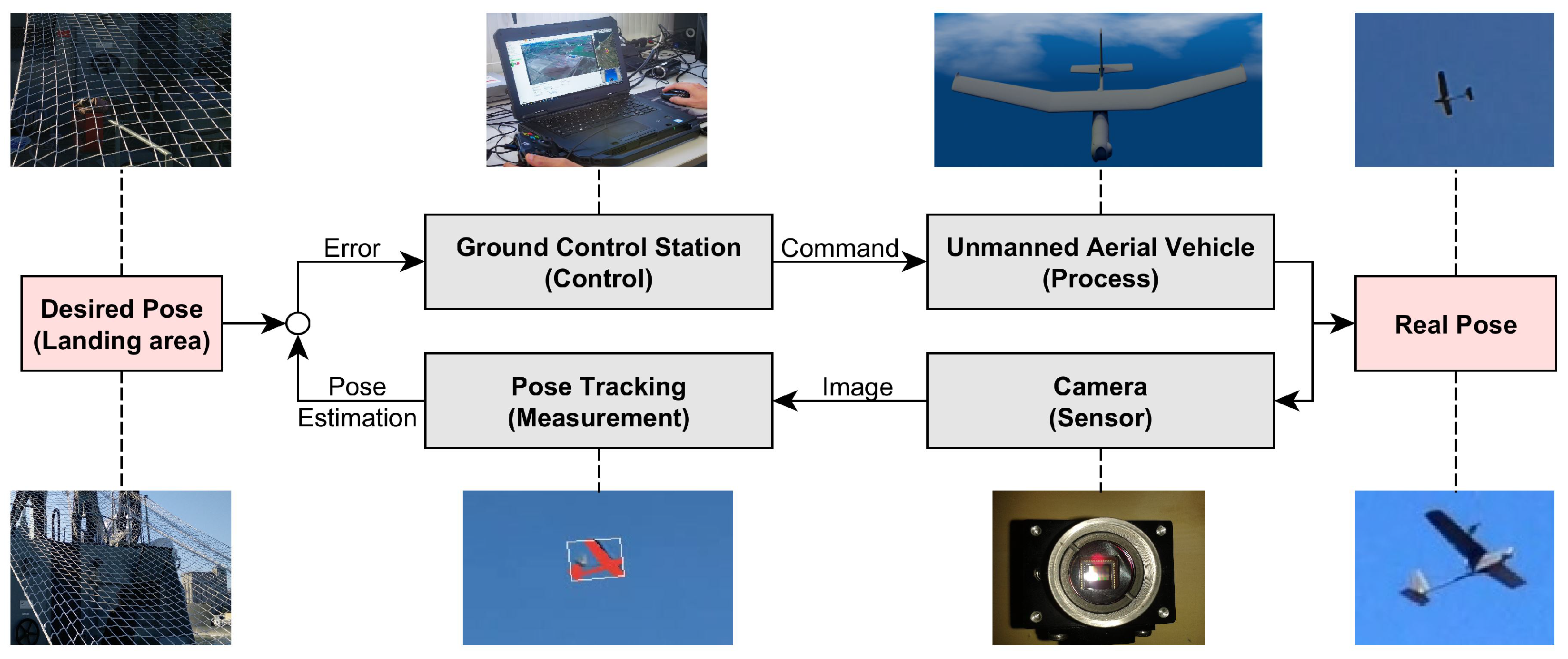
An autonomous landing system’s final objective is to use the sensor information to control the trajectory of the UAV. In this article, the main focus was on the use of the camera information (sensor) to perform pose tracking (measurement) over time (Figure 4).
We used a ground-based monocular RGB camera system to sense the real world (capture image frames), using a frame rate of 30 Frames Per Second (FPS) and an image size of pixels (width × height) [11,35]. Then, we combined that information with algorithms that use the UAV CAD model as a priori information. In this specific application, the camera should be located near the landing area to be able to estimate the UAV’s relative pose to the camera (translation and orientation) and perform tracking (Figure 5).
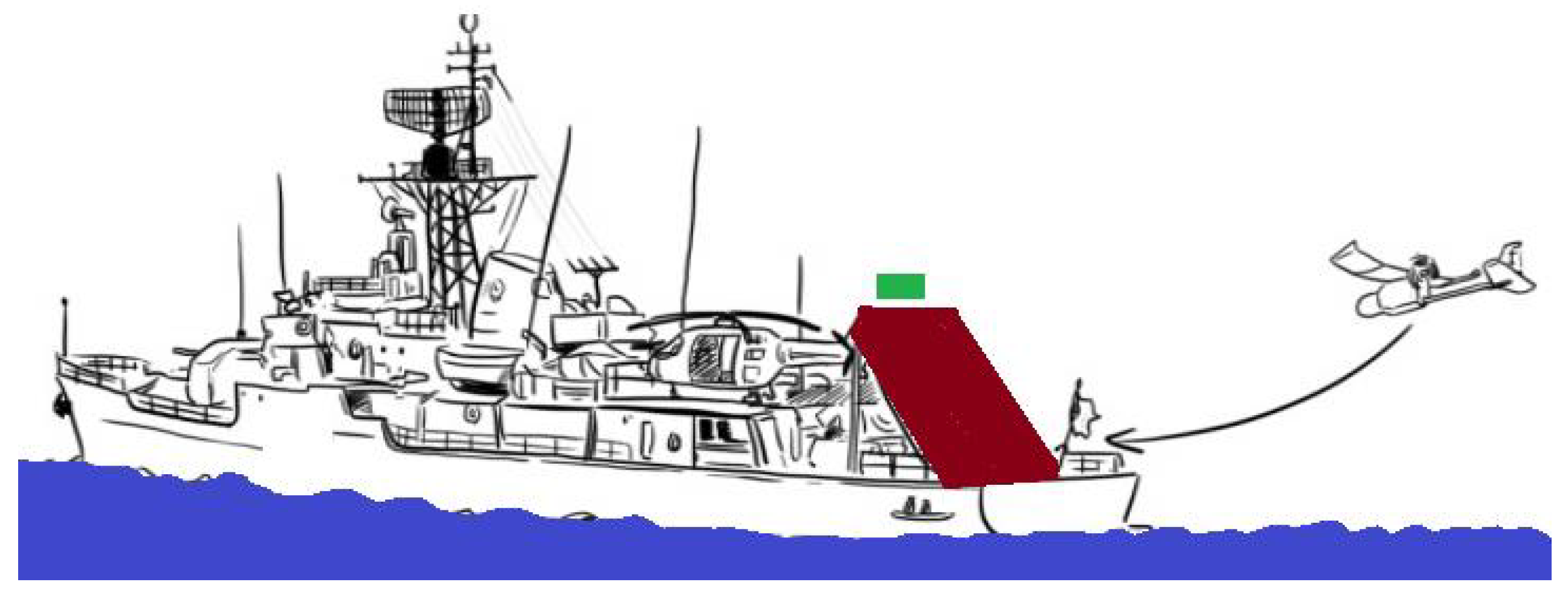
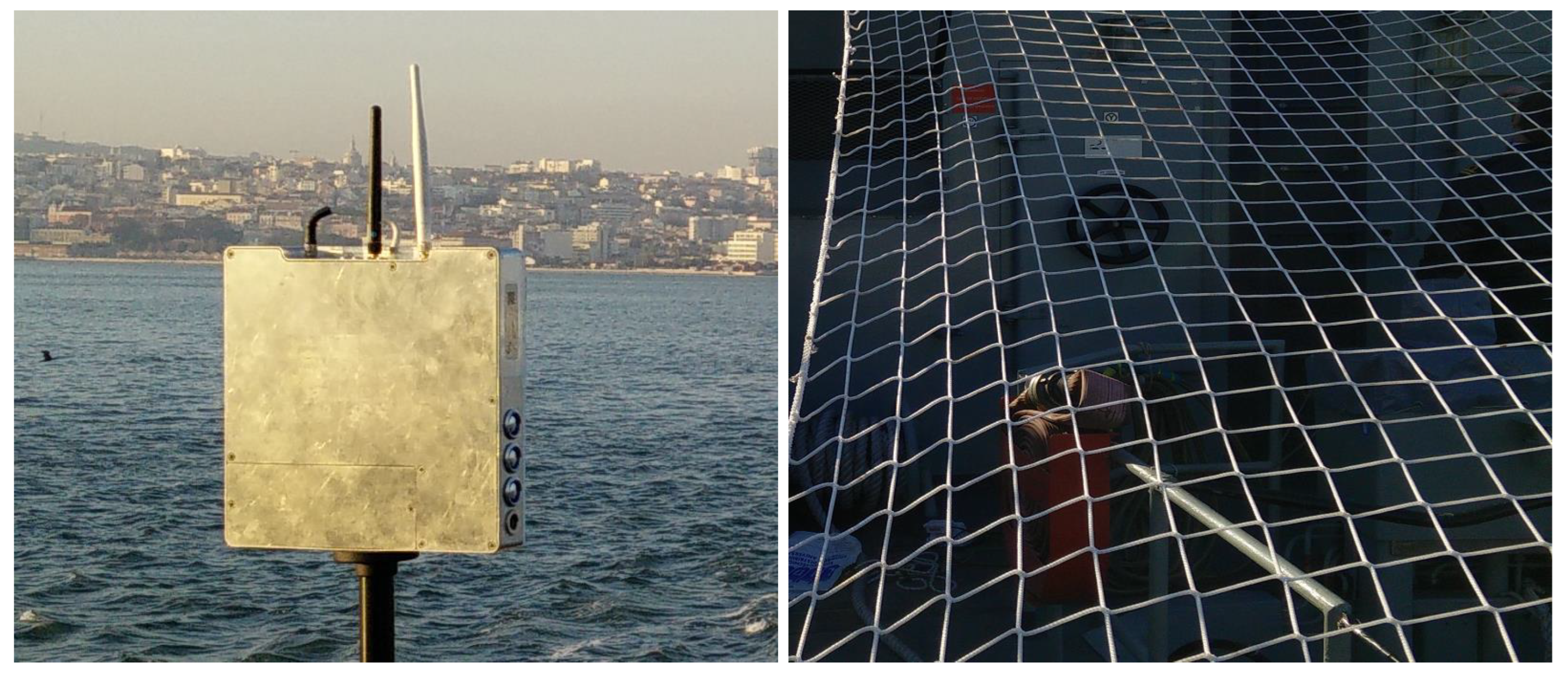
Additionally, we only need to ensure communication with the UAV to send the needed trajectories to a simple onboard autopilot and to ensure also that the net-based retention system is installed and that it has the needed characteristics to ensure no damage to the UAV or ship (Figure 6). In a small-sized FPB, the expected landing area (net-based retention system available landing area) is about m, which is about 2.5-times larger than the used UAV model’s wingspan (Table 1).
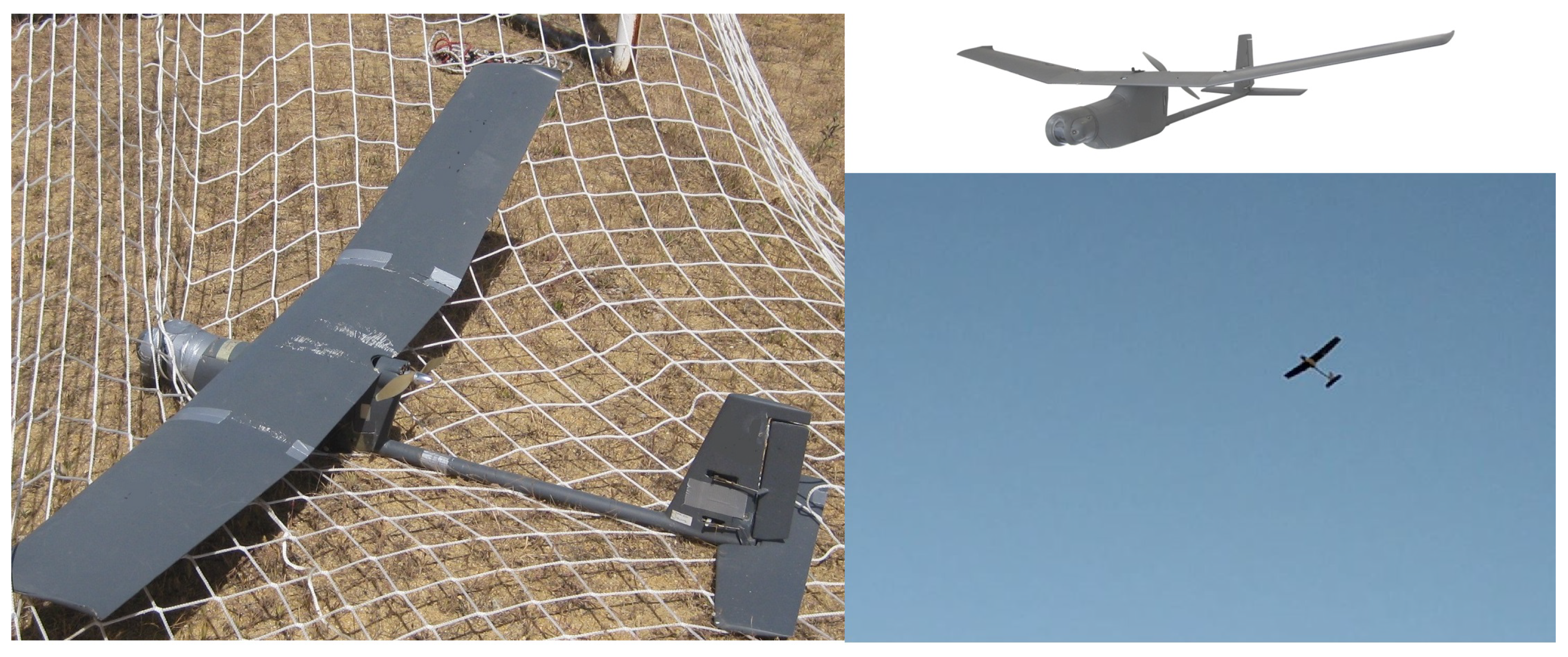
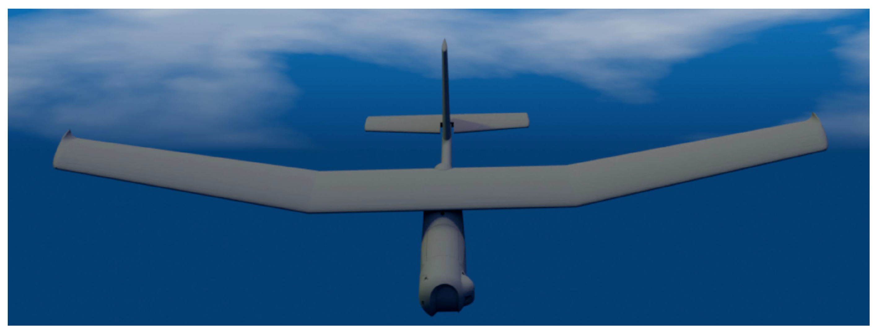
We used a small-sized fixed-wing UAV (Figure 7), with the characteristics described in Table 1. Due to its size and weight, the UAV’s take-off can be easily performed by hand, and all the focus will be on the landing maneuver, as described before. It is essential to develop autonomous methods that are more reliable than using a human-in-the-loop, being able to decrease the probability of an accident.
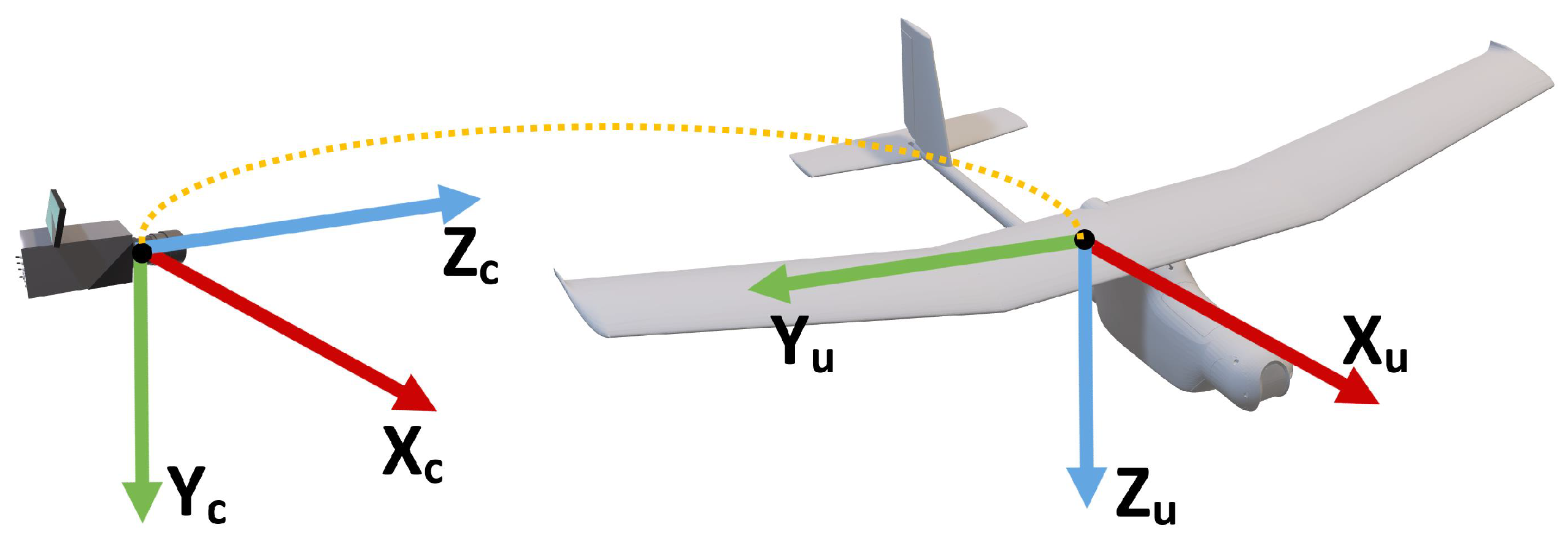
During the development of the adopted approach, we considered that (i) the UAV is a rigid body; (ii) the UAV’s mass and mass distribution remain constant during operation; (iii) the UAV’s reference frame origin is located in its Center Of Gravity (COG). The UAV’s state is represented according to the camera reference frame according to [41]:
where is the linear position, is the linear velocity, is the angular orientation (quaternion representation), and is the angular velocity according to the camera reference frame represented in Figure 8.
As described initially in Section 1, the proposed tracking architecture is divided into (Figure 9) [41,42,43,87]:
- Pose Boosting (Section 3.1)—In this stage, the UAV is detected in the captured frame using deep learning, and filter initialization is performed using a pre-trained database. In each iteration, information from the current frame (using the pre-trained database) using the most-current observation to add particle diversity is also used;
- Tracking (Section 3.2)—In this stage, we used a 3D-model-based approach based on a PF to perform tracking. By applying temporal filtering, we improved the accuracy by being able to minimize the estimation error;
- Pose Optimization (Section 3.3)—Since we used a similarity metric to obtain the particle weights, we added a refinement step that uses the current frame (current time instant) and the current estimate to search for a better solution.
3.1. Pose Boosting
This stage was initially inspired by the Boosted Particle Filter (BPF) [88], which extends the Mixture Particle Filter (MPF) application [89] by incorporating Adaptive Boosting (AdaBoost) [90]. We adopted the approach described in [41,42,43,87], characterized by the following two stages:
- Detection—In this stage, we detect the UAV in the captured frame using the You Only Look Once (YOLO) [91] object detector. Target detection is critical since we were operating in an outdoor environment and we can be in the presence of other objects that can affect the system’s reliability;
- Hypotheses generation—From the ROIs obtained in the detection stage, we cannot infer the UAV’s orientation, but only its 3D position. To deal with this, we obtained the UAV’s Oriented Bounding Box (OBB) and performed the comparison with a pre-trained database of synthetically generated poses to obtain the pose estimates (Figure 10).
3.2. Tracking
We adopted a PF approach based on the Unscented Particle Filter (UPF) [92], whose standard scheme is divided into three stages: (i) initialization, (ii) importance sampling, and (iii) importance weighting and resampling. The initialization was performed in the pose boosting stage described in Section 3.1. The main difference, when compared with the standard UKF is in the importance sampling stage, where we used a UKF for the translational motion and a UBiF/UBiGaF for the rotational motion to be able to incorporate the current observation and generate a better proposal distribution. The adopted tracking stage is divided into the following two stages [41,42]:
- Proposal (Section 3.2.1)—In this stage, we generate the proposal distribution, which should be as close as possible to the true posterior distribution;
- Approximate weighting and resampling (Section 3.2.2)—In this stage, we approximate the particle weights (approximate weighting) by using a Distance-Transform-based similarity metric. After evaluating the particles, we apply a resampling scheme to replicate the high-weight ones and eliminate the low-weight ones.
3.2.1. Proposal
Motion filtering has the purpose of using measures affected by uncertainty over time and being able to generate results closer to reality. We adopted the motion model (translational and rotational model) described in [12,41,42], where a UKF is applied to the translational filtering and a UBiF/UBiGaF to the rotational filtering. The Bingham (Bi) distribution is an antipodally symmetric distribution [93] used by the UBiF to better quantify the existing uncertainty without correlation between angular velocity and attitude. On the other hand, the UBiGaF uses a Bingham–Gauss (BiGa) [45] distribution, which takes into account this uncertainty in the filtering structure. The UBiF update step is simple to implement since the product between two Bi distributions is closed after renormalization. Still, the same does not happen in the BiGa distribution, which needs to have an update step based on the Unscented Transform (UT) [42,45,94]. We already explored both implementations in [12,41,42], it being possible to state that we have a clear performance improvement when compared with traditional methods, e.g., the UKF.
3.2.2. Approximate Weighting and Resampling
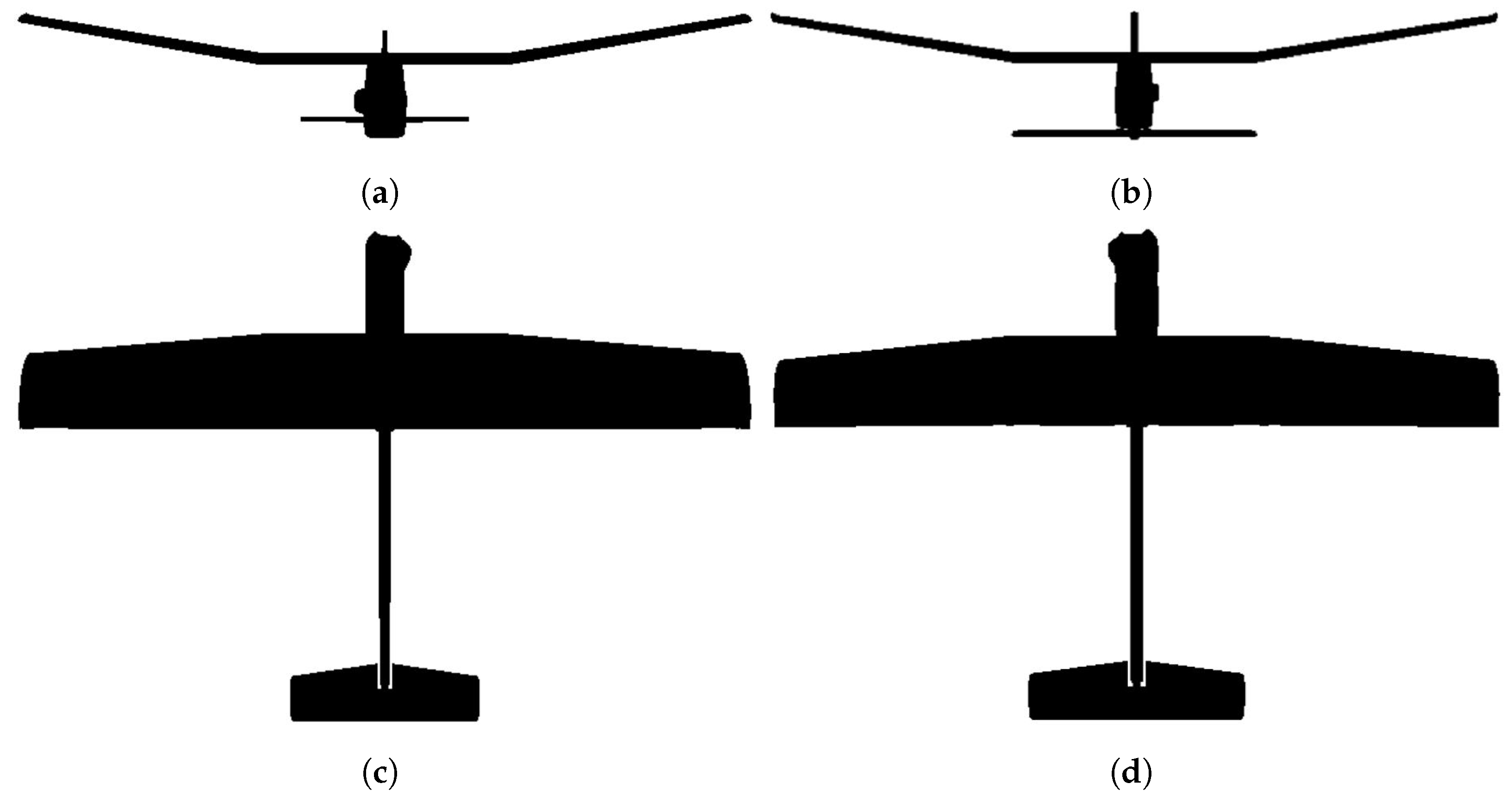
Usually, the object characteristics and the search space complexity are the primary sources of complexity in tracking. We used a small-size fixed-wing UAV (Figure 11), which is very difficult to detect at long distances since it is designed for military surveillance operations. On the other hand, the vast search space is outdoors, making the problem very complex, since we wanted to start detecting the UAV at least 80 m from the landing area.
The UAV model symmetries are another problem since we used a 3D-model-based approach, where we need clearly to discriminate in the captured frame the correct UAV pose. In Figure 12, we see that symmetric poses have almost the same appearance, affecting the obtained results since we used a pixel-based similarity metric. The angle represents the rotation around the camera x-axis; the angle represents the rotation around the camera y-axis; the angle represents the rotation around the camera z-axis, as described in Figure 8. In this article, we implemented the Distance Transform (DT) similarity metric described in [43,95]. This similarity metric computes the distance to the closest edge between the DT [96] of the captured frame and the edge map [97] of the pose hypothesis to compare. The DT similarity metric is obtained according to:
where is a fine-tuning parameter and s is given by
where k is the number of edge pixels of the hypothesis to compare, B is the total number of image pixels, h is the pose hypothesis image, f is the captured frame, is the DT of the captured frame, and is the edge map of the pose hypothesis image to compare.
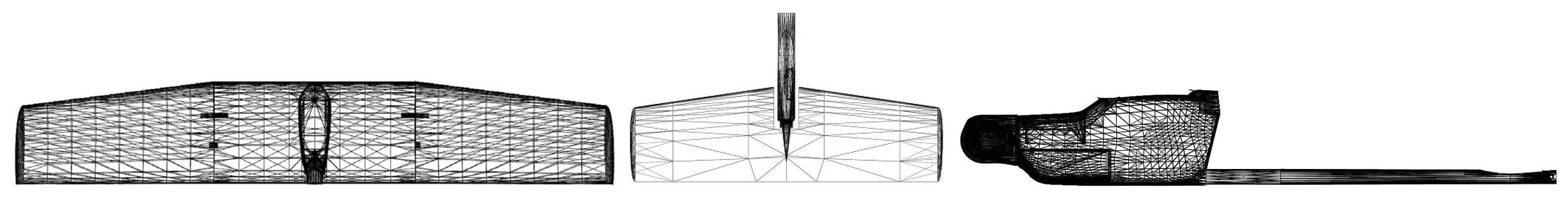
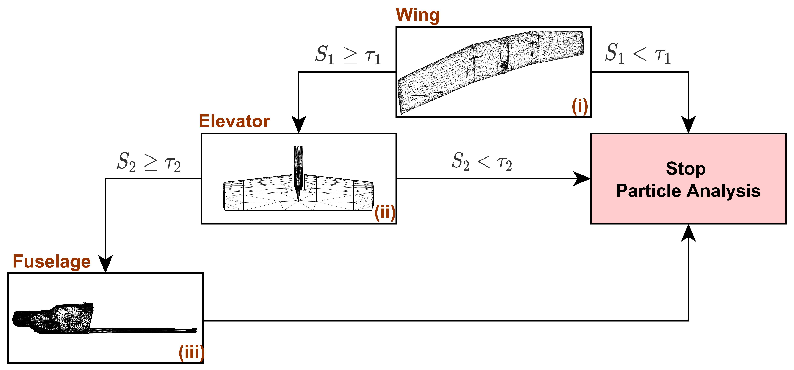
Some of the most time-demanding operations in 3D-model-based pose estimation are particle rendering (pose hypothesis rendering) and evaluation [35]. Considering that, at each instant (system iteration), we evaluated hundreds of particles (or even thousands), we realized that we needed to optimize these operations. A complex problem to be solved is normally divided into smaller ones, and the same approach was adopted here regarding the UAV CAD model. We divided the UAV CAD model into the following smaller parts (Figure 13): (i) wing, (ii) elevator, and (iii) body. Since the adopted similarity metric can be computed independently for each UAV part, we can adopt a particle evaluation strategy where each part is evaluated independently. If needed, discard the evaluation sooner, or combine the obtained weights.
To optimize the particle evaluation, a tree-based similarity metric approach is used (Figure 14), where each part is evaluated independently and sequentially (wing, elevator, and then, fuselage) compared with a predefined threshold (which can be different for each part). If the obtained weight S is smaller than a predefined threshold, the analysis avoids rendering the complete UAV CAD model. This allows us to use the available processing power better, only performing a complete model rendering and analysis for the promising particles. The adopted tree-based similarity metric for each particle is given by
where are fine-tuning parameters, is the DT similarity metric for the wing part, is the DT similarity metric for the elevator part, and is the DT similarity metric for the fuselage part. By adjusting the threshold levels and the fine-tuning parameters, we can guarantee that the sum of the evaluations is equivalent to the evaluation of the whole model alone. This method can speed up the particle evaluation without a loss in accuracy.
3.3. Pose Optimization
In this stage, we performed a local search (refinement steps) in the particle neighborhood to optimize the used similarity metric using the current frame information. The adopted similarity metric is multimodal with more than one peak and cannot be optimized using gradient-based methods [41,43]. We adopted the Particle Filter Optimization (PFO) approach described in [43], which is based on the PF theory, but uses the same input (image frame) in each iteration. Using a zero velocity model, the PFO method is similar to a PF applied repetitively in the same frame. By adjusting the added noise to decrease over time, we can obtain better estimates and reduce the needed convergence time.
4. Experimental Results
This section describes the experimental results, in particular the tests (Section 4.1), the analyzed synthetic sequence (Section 4.2), the adopted performance metrics (Section 4.3), and the obtained pose tracking results (Section 4.4).
The method was initially implemented on a 3.70 GHz Intel i7-8700K Central Processing Unit (CPU) and NVIDIA Quadro P5000 with a bandwidth of 288.5 GB/s and a pixel rate of 110.9 GPixel/s. If we need to render and process 100 particles using the proposed filters, we will obtain approximately 27 FPS [9,13], which is a performance suitable for a real-time application [9,13,34,41,42,87]. Since we used a ground-based system without any power limitations and easy access to high processing capabilities, the obtained processing time was expected to be lower than the one described here.
4.1. Tests’ Description
The experimental tests described in Section 4.4 aimed to quantify the system’s performance, considering the similar metric analysis and the obtained pose estimation error in a realistic synthetic dataset (Section 4.2). Taking this into account, three different tests were performed with the following objectives:
- Similarity metric analysis (Section 4.4.1)—In this test, we had the objective of evaluating the tree-based similarity metric approach and comparing it with the standard DT similarity metric;
- Pose tracking without pose optimization (Section 4.4.2)—In this test, we had the objective of comparing the two filtering approaches when changing the number of used particles;
- Pose tracking with pose optimization (Section 4.4.3)—In this test, we had the objective of comparing the two filtering approaches when changing the number of pose optimization iterations using a constant number of particles.
4.2. Synthetic Sequence
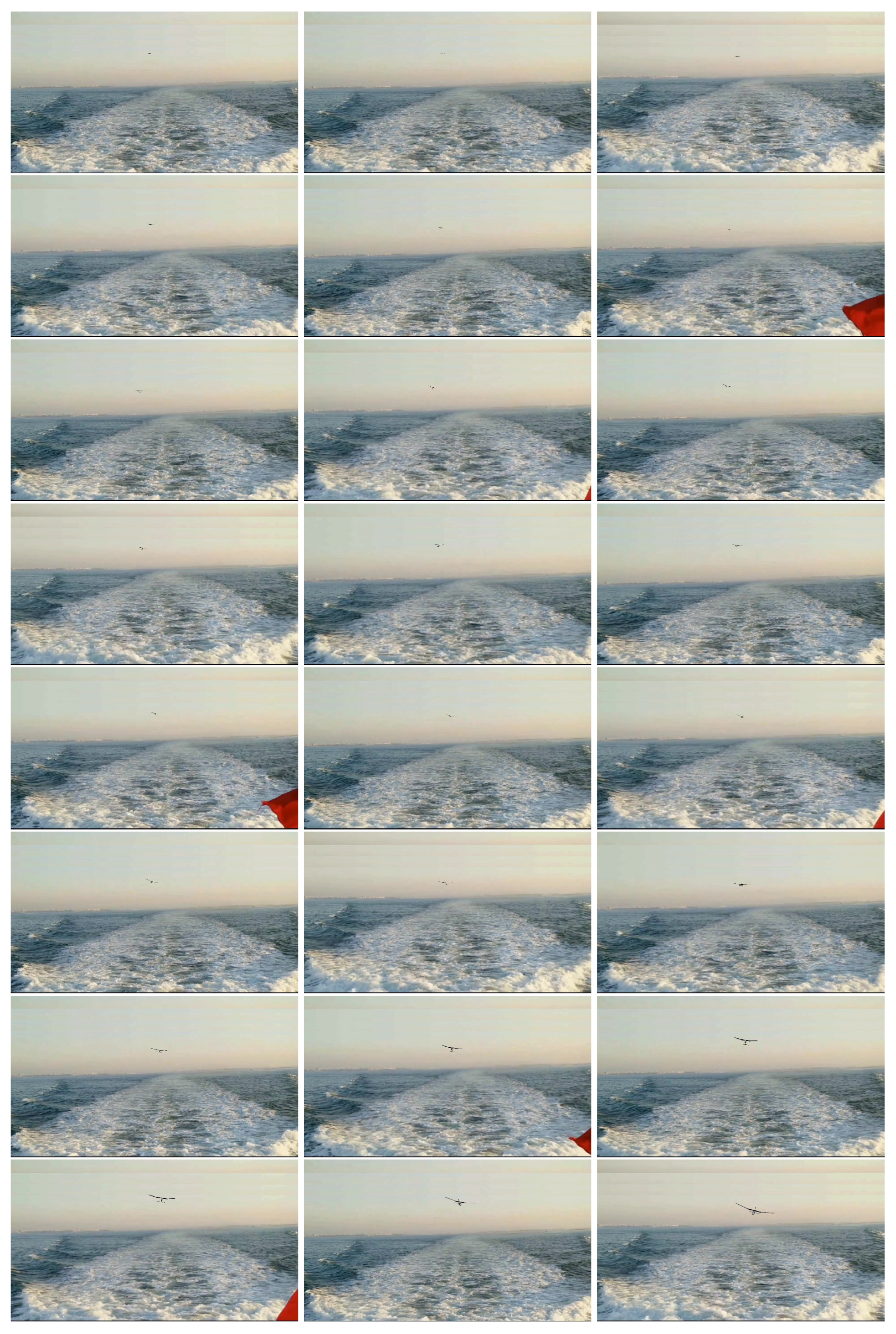
Since there is no publicly available dataset and we could not acquire an actual image dataset until now, we used a realistic synthetic dataset (Figure 15). Based on some obtained experimental data, a UAV trajectory (translation and rotation) was created to be able to test the developed algorithms, as described in Figure 16. This landing sequence represents the expected trajectory of a landing UAV on an FPB.
4.3. Performance Metrics
The particle with the highest weight value gives the UAV’s pose on each iteration before resampling. The translational error is given by the Euclidean error, and the rotation error is obtained according to
where is the ground truth rotation matrix and corresponds to the retrieved rotation matrices (possibilities). We also obtained the Mean Absolute Error (MAE), Root-Mean-Squared Error (RMSE), and Standard Deviation (SD) to be able to perform a better performance analysis.
4.4. Pose Tracking
Since the knowledge has to be cumulative, the adopted filter parameters were the same as described in [42], allowing a performance comparison with the obtained experimental results. It is essential to consider that, in the implementation described in [42], a different similarity metric was used, and no pose optimization scheme was not used.
4.4.1. Similarity Metric Analysis
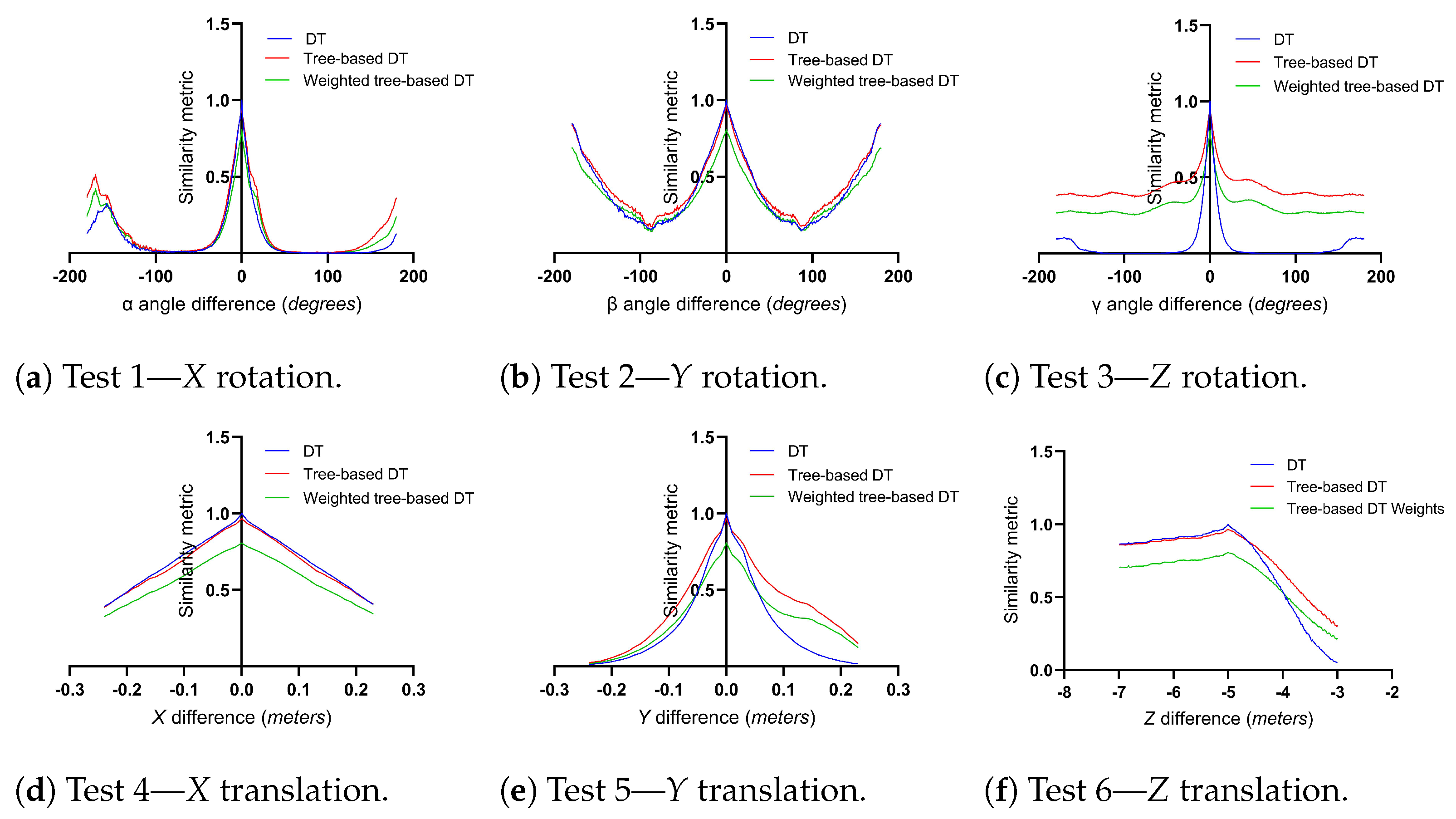
To be able to assess the pose evaluation performance, we performed six different tests (Table 2) on three different similarity metric approaches: (i) DT, (ii) tree-based DT, and (iii) weighted-tree-based DT (, , and ).
After analyzing Figure 17, it is possible to see that the standard DT transform similarity metric obtained almost the same results as the tree-based DT approach. With a small change in the tuning coefficients (), it is possible to adapt the output better, as described in Figure 17. The tree-based DT approach generated results close to the standard DT similarity metric. It can be used without increasing the error obtained, decreasing the particle evaluation processing time.
4.4.2. Pose Tracking without Pose Optimization
The translation estimate error decreased with the increase of the particle number (Table 3 and Table 4). Although we used the UKF in both implementations for the translation estimation (UBiF and UBiGaF) since the orientation also influences the similarity metric value, we obtained better translation results in the UBiGaF case.
Regarding rotation, the best compromise between speed and accuracy (particle number vs. obtained results) was obtained when using 100 particles (Table 5 and Table 6). The UBiF obtained better results when compared to the UBiGaF. Nevertheless, both filters obtained very good results given the realistic representation given by the used synthetic environment.
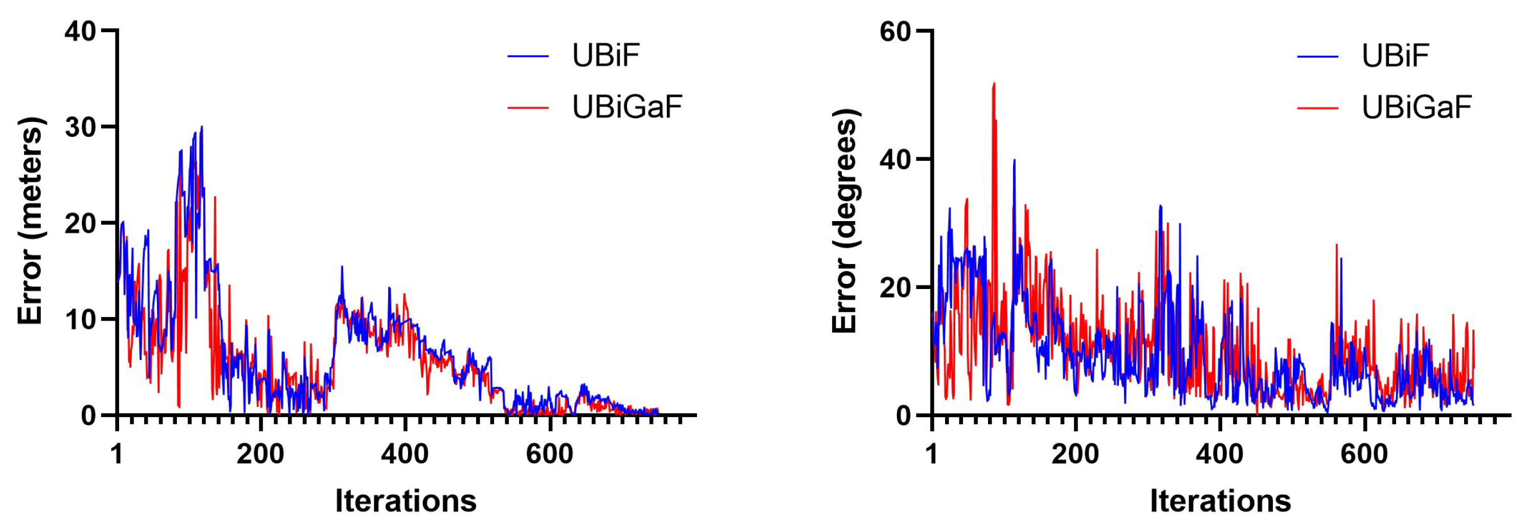
The comparison between the Euclidean error and the rotation error for the UBiF and UBiGaF when using 100 particles can be seen in Figure 18. Both filter implementations had some associated error, with higher variations given by the UBiGaF implementation. This happened mainly due to the correlation between the orientation and the angular velocity, making the output noisier (Figure 19).
4.4.3. Pose Tracking with Pose Optimization
In this test, we used 100 particles, which corresponded to the best-obtained results described in the previous subsection, and changed the number of pose optimization iterations. The translation estimate error decreased with the increase of the pose optimization iterations (Table 7 and Table 8). Although we used the UKF in both implementations for the translation estimation (UBiF and UBiGaF), we also obtained better results in the UBiGaF case.
Regarding rotation, the best compromise between speed and accuracy was obtained using two pose optimization iterations (Table 9 and Table 10). We can see some refinement in the obtained results, and we obtained better results when using pose optimization when compared with the particle number increase. We increased the algorithm’s accuracy by searching locally for a better solution. Combined with the tree-based DT similarity metric, this decreased the obtained error and the needed processing time.
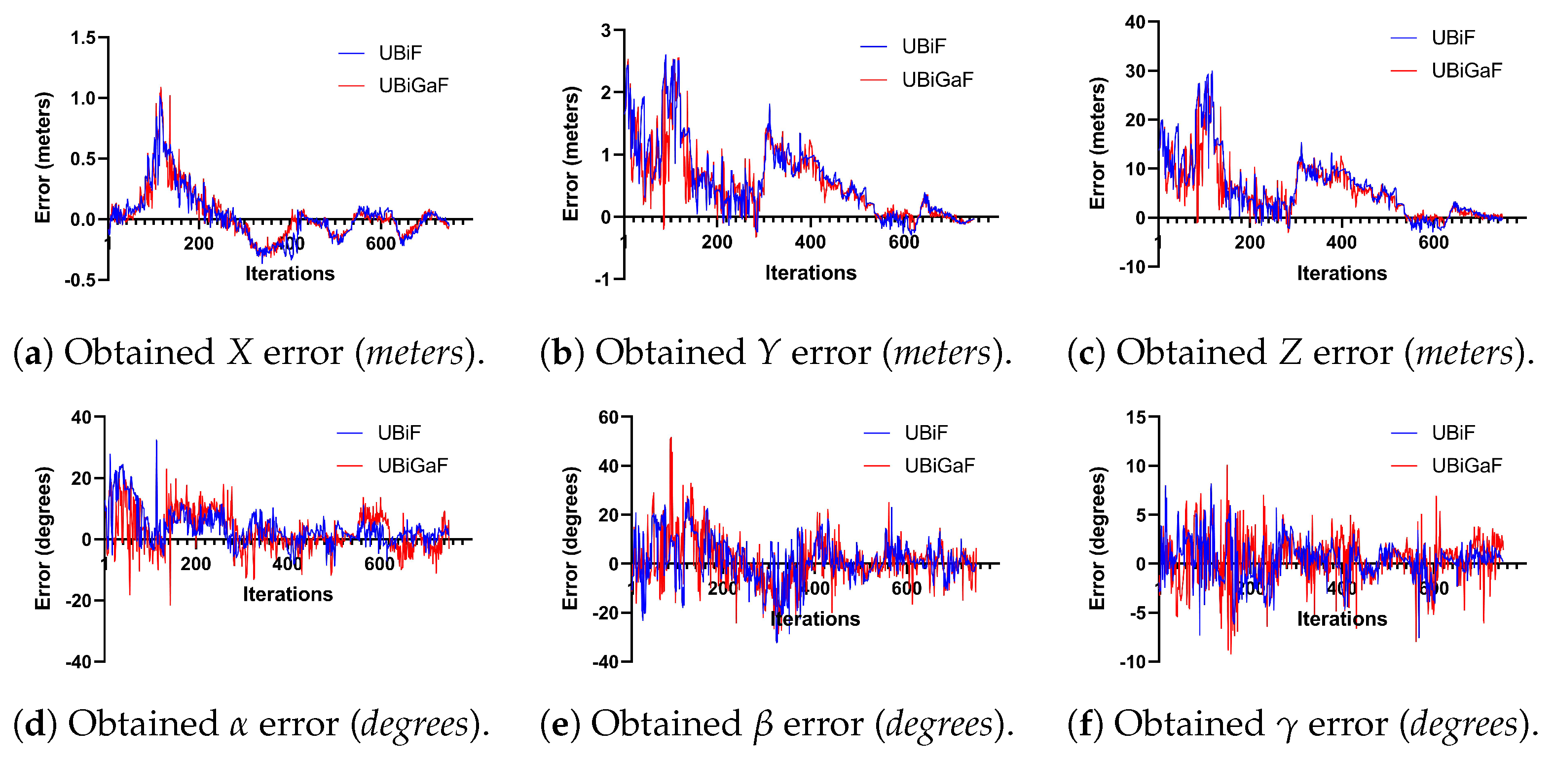
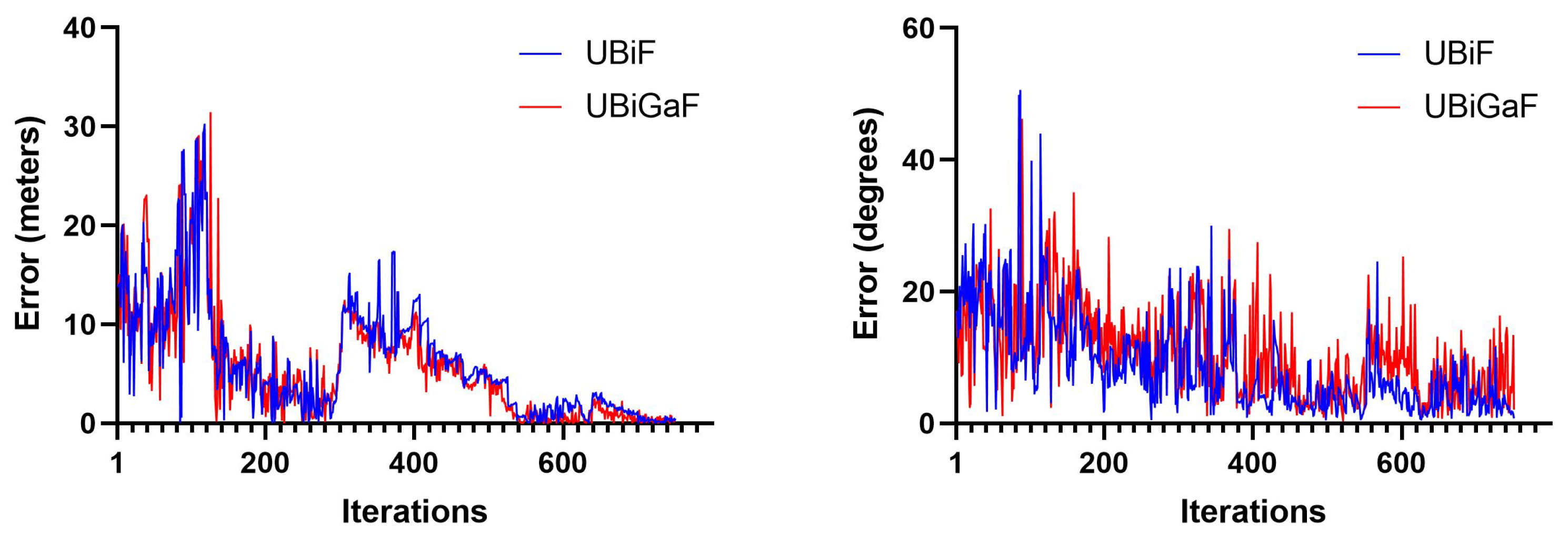
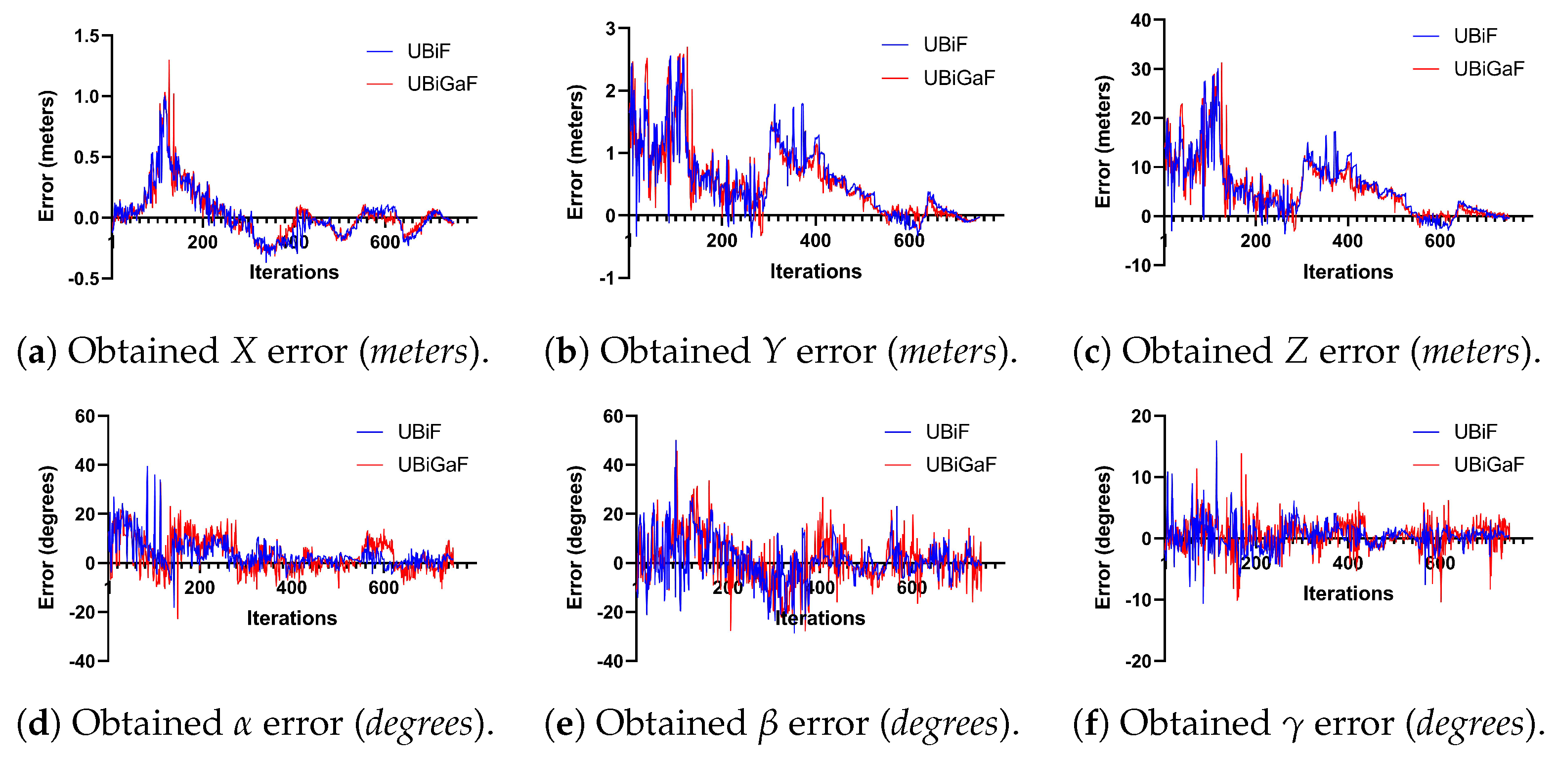
The comparison between the Euclidean error and the rotation error for the UBiF and UBiGaF when using 100 particles and two pose optimization iterations can be seen in Figure 20. Both filter implementations had some associated errors, with some variations, but they were a bit smoother than those shown in the previous subsection.
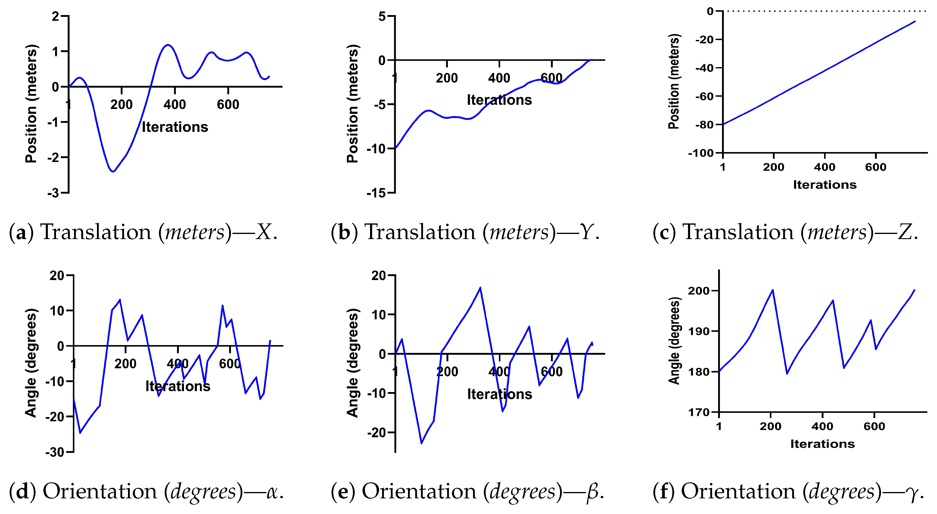
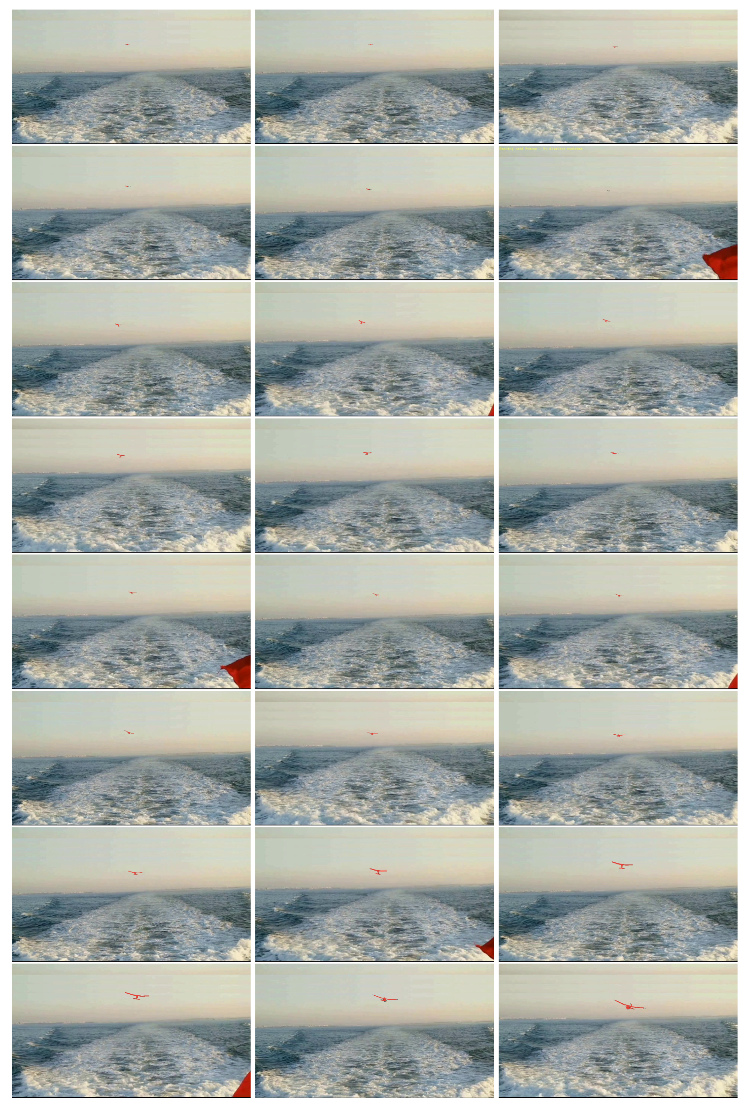
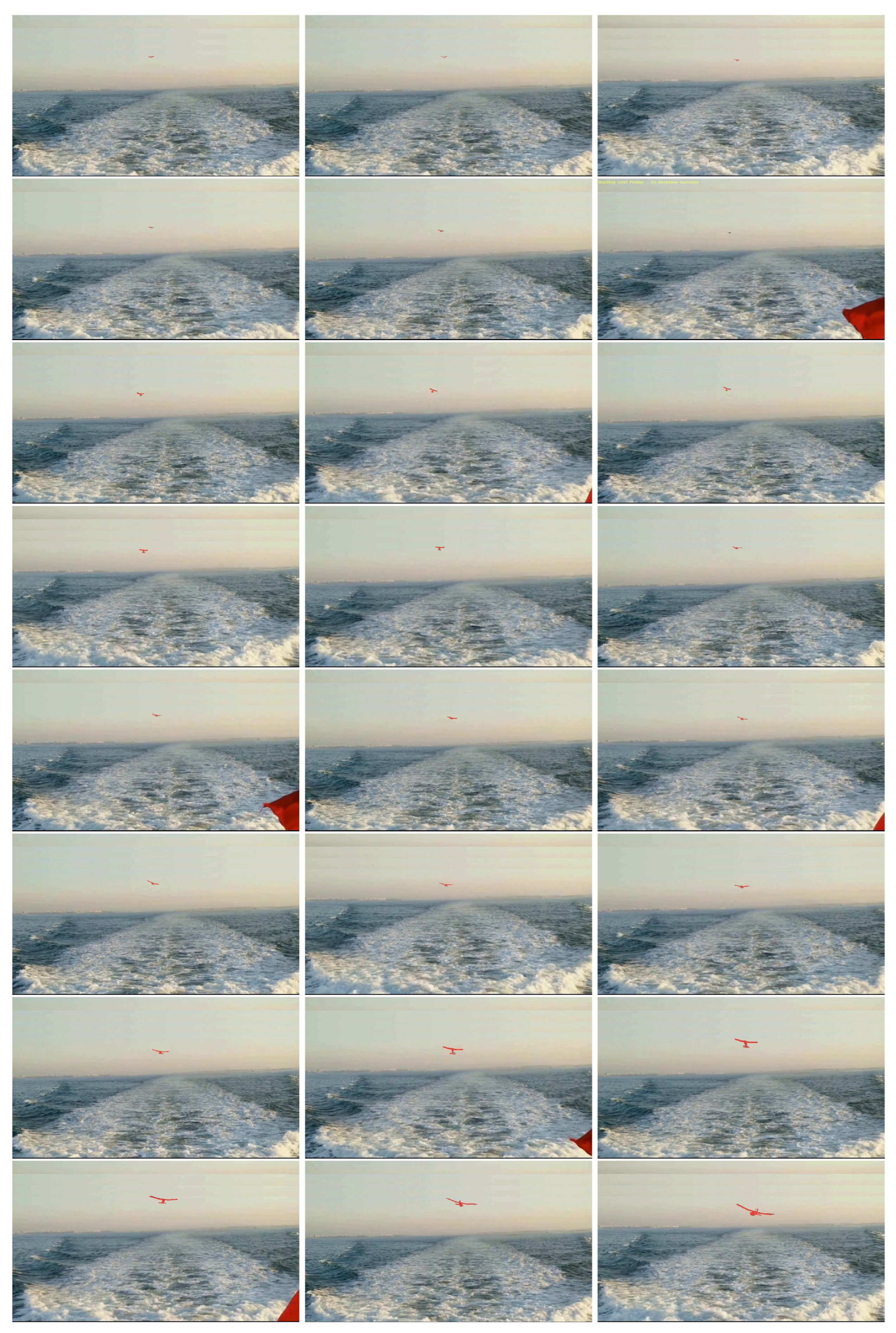
Figure 21 describes in detail the obtained translation and rotation errors, and it is possible to see that the UBiGaF presented fewer jumps in the orientation estimation when compared with the UBiF when using pose optimization. This was a clear difference and improvement in performance when compared with the results obtained in the previous subsection. The results obtained when implementing these methods can be seen in Figure 22 and Figure 23, where the estimated pose obtained is represented in red.
5. Conclusions and Future Work
It is expected to obtain better estimates and achieve real-time implementation by continuously improving and exploring the developed system. Directional statistics are critical to represent the orientation better since we can obtain lower estimation errors. In a world wholly taken over by deep learning approaches, it is essential to continue to explore more traditional techniques, continuously developing the knowledge in the field. The 3D-model-based tracking approach is not simple, especially outdoors, where we cannot control the environmental conditions. The similarity metric was not based on specific color information, but directly on the DT calculation to deal with that design constraint. The similarity metric decreased the processing time without a loss in the accuracy of the result. The obtained translation and rotation errors decreased with the UAV’s proximity to the camera since we had more pixel information. The obtained errors were compatible with the automatic landing requirements since we expected a minimum available landing area of 5 meters. This area is typically available in a small patrol boat that performs surveillance tasks or even conducts search and rescue operations. Future work will focus on improving the algorithm’s accuracy and obtaining a real dataset that can be used to improve the algorithm. This work will also contribute to developing other works in the field, since we plan to make it publicly available.
Author Contributions
Conceptualization, N.P.S., V.L. and A.B.; methodology, N.P.S. and A.B.; software, N.P.S.; validation, N.P.S. and A.B.; formal analysis, N.P.S. and A.B.; investigation, N.P.S.; resources, N.P.S.; data curation, N.P.S.; writing—original draft preparation, N.P.S.; writing—review and editing, N.P.S.; visualization, N.P.S.; supervision, N.P.S.; project administration, N.P.S.; funding acquisition, Not applicable. All authors have read and agreed to the published version of the manuscript.
Funding
This research received no external funding.
Data Availability Statement
The manuscript includes all the data and materials supporting the presented conclusions.
Conflicts of Interest
The authors declare no conflict of interest.
References
- Cabrita, M.T.; Silva, A.; Oliveira, P.B.; Angélico, M.M.; Nogueira, M. Assessing eutrophication in the Portuguese continental Exclusive Economic Zone within the European Marine Strategy Framework Directive. Ecol. Indic. 2015, 58, 286–299. [Google Scholar] [CrossRef]
- Calado, H.; Bentz, J. The Portuguese maritime spatial plan. Mar. Policy 2013, 42, 325–333. [Google Scholar] [CrossRef]
- Hoagland, P.; Jacoby, J.; Schumacher, M. Law Of The Sea. In Encyclopedia of Ocean Sciences; Steele, J.H., Ed.; Academic Press: Oxford, UK, 2001; pp. 1481–1492. [Google Scholar] [CrossRef]
- Stasolla, M.; Mallorqui, J.J.; Margarit, G.; Santamaria, C.; Walker, N. A Comparative Study of Operational Vessel Detectors for Maritime Surveillance Using Satellite-Borne Synthetic Aperture Radar. IEEE J. Sel. Top. Appl. Earth Obs. Remote Sens. 2016, 9, 2687–2701. [Google Scholar] [CrossRef] [Green Version]
- Ma, S.; Wang, J.; Meng, X.; Wang, J. A vessel positioning algorithm based on satellite automatic identification system. J. Electr. Comput. Eng. 2017, 2017, 8097187. [Google Scholar] [CrossRef] [Green Version]
- Marzuki, M.I.; Gaspar, P.; Garello, R.; Kerbaol, V.; Fablet, R. Fishing Gear Identification From Vessel-Monitoring-System-Based Fishing Vessel Trajectories. IEEE J. Ocean. Eng. 2018, 43, 689–699. [Google Scholar] [CrossRef]
- Rowlands, G.; Brown, J.; Soule, B.; Boluda, P.T.; Rogers, A.D. Satellite surveillance of fishing vessel activity in the Ascension Island Exclusive Economic Zone and Marine Protected Area. Mar. Policy 2019, 101, 39–50. [Google Scholar] [CrossRef]
- Wang, R.; Shao, S.; An, M.; Li, J.; Wang, S.; Xu, X. Soft Thresholding Attention Network for Adaptive Feature Denoising in SAR Ship Detection. IEEE Access 2021, 9, 29090–29105. [Google Scholar] [CrossRef]
- Pessanha Santos, N.; Melicio, F.; Lobo, V.; Bernardino, A. A Ground-Based Vision System for UAV Pose Estimation. Int. J. Mechatronics Robot.-(IJMR)–Unsysdigital Int. J. 2014, 1, 7. [Google Scholar]
- Goncalves-Coelho, A.M.; Veloso, L.C.; Lobo, V.J.A.S. Tests of a light UAV for naval surveillance. In Proceedings of the OCEANS 2007—Europe, Aberdeen, UK, 18–21 June 2007; pp. 1–4. [Google Scholar] [CrossRef]
- Pessanha Santos, N.; Lobo, V.; Bernardino, A. AUTOLAND project: Fixed-wing UAV Landing on a Fast Patrol Boat using Computer Vision. In Proceedings of the OCEANS 2019—Seattle, Seattle, WA, USA, 27–31 October 2019. [Google Scholar] [CrossRef]
- Pessanha Santos, N.; Lobo, V.; Bernardino, A. A Ground-Based Vision System for UAV Tracking. In Proceedings of the OCEANS 2015, Genova, Italy, 18–21 May 2015. [Google Scholar] [CrossRef]
- Pessanha Santos, N.; Lobo, V.; Bernardino, A. Particle Filtering based optimization applied to 3D-model-based estimation for UAV pose estimation. In Proceedings of the OCEANS 2017, Aberdeen, UK, 19–22 June 2017. [Google Scholar] [CrossRef]
- Iscold, P.; Pereira, G.A.S.; Torres, L.A.B. Development of a Hand-Launched Small UAV for Ground Reconnaissance. IEEE Trans. Aerosp. Electron. Syst. 2010, 46, 335–348. [Google Scholar] [CrossRef]
- Manning, S.D.; Rash, C.E.; Leduc, P.A.; Noback, R.K.; McKeon, J. The Role of Human Causal Factors in US Army Unmanned Aerial Vehicle Accidents; Technical Report; Army Aeromedical Research Lab: Fort Rucker, AL, USA, 2004. [Google Scholar]
- Williams, K.W. A Summary of Unmanned Aircraft Accident/Incident Data: Human Factors Implications; Technical Report; Federal Aviation Administration Civil Aerospace Medical Institute: Oklahoma, OK, USA, 2004. [Google Scholar]
- Williams, K.W. 8. Human Factors Implications of Unmanned Aircraft Accidents: Flight-Control Problems. In Human Factors of Remotely Operated Vehicles; Emerald Group Publishing Limited.: Bingley, UK, 2006; Volume 7, pp. 105–116. [Google Scholar]
- Waraich, Q.R.; Mazzuchi, T.A.; Sarkani, S.; Rico, D.F. Minimizing Human Factors Mishaps in Unmanned Aircraft Systems. Ergon. Des. 2013, 21, 25–32. [Google Scholar] [CrossRef]
- Agbeyangi, A.O.; Odiete, J.O.; Olorunlomerue, A.B. Review on UAVs used for aerial surveillance. J. Multidiscip. Eng. Sci. Technol. 2016, 3, 5713–5719. [Google Scholar]
- Abiodun, T.F. Usage of drones or unmanned aerial vehicles (UAVs) for effective aerial surveillance, mapping system and intelligence gathering in combating insecurity in Nigeria. Afr. J. Soc. Sci. Humanit. Res. 2020, 3, 29–44. [Google Scholar]
- Morais, F.; Ramalho, T.; Sinogas, P.; Monteiro Marques, M.; Pessanha Santos, N.; Lobo, V. Trajectory and guidance mode for autonomously landing a UAV on a naval platform using a vision approach. In Proceedings of the OCEANS 2015, Genova, Italy, 18–21 May 2015; pp. 1–7. [Google Scholar] [CrossRef]
- Skulstad, R.; Syversen, C.; Merz, M.; Sokolova, N.; Fossen, T.; Johansen, T. Autonomous net recovery of fixed-wing UAV with single-frequency carrier-phase differential GNSS. IEEE Aerosp. Electron. Syst. Mag. 2015, 30, 18–27. [Google Scholar] [CrossRef]
- Paredes, J.; Sharma, P.; Ha, B.; Lanchares, M.; Atkins, E.; Gaskell, P.; Kolmanovsky, I. Development, implementation, and experimental outdoor evaluation of quadcopter controllers for computationally limited embedded systems. Annu. Rev. Control 2021, 52, 372–389. [Google Scholar] [CrossRef]
- Klausen, K.; Fossen, T.I.; Johansen, T.A. Autonomous recovery of a fixed-wing UAV using a net suspended by two multirotor UAVs. J. Field Robot. 2018, 35, 717–731. [Google Scholar] [CrossRef]
- Bornebusch, M.F.; Johansen, T.A. Autonomous Recovery of a Fixed-Wing UAV Using a Line Suspended Between Two Multirotor UAVs. IEEE Trans. Aerosp. Electron. Syst. 2021, 57, 90–104. [Google Scholar] [CrossRef]
- Lee, C.; Kim, S.; Chu, B. A survey: Flight mechanism and mechanical structure of the UAV. Int. J. Precis. Eng. Manuf. 2021, 22, 719–743. [Google Scholar] [CrossRef]
- Goh, G.; Agarwala, S.; Goh, G.; Dikshit, V.; Sing, S.; Yeong, W. Additive manufacturing in unmanned aerial vehicles (UAVs): Challenges and potential. Aerosp. Sci. Technol. 2017, 63, 140–151. [Google Scholar] [CrossRef]
- Leira, F.S.; Trnka, K.; Fossen, T.I.; Johansen, T.A. A ligth-weight thermal camera payload with georeferencing capabilities for small fixed-wing UAVs. In Proceedings of the 2015 International Conference on Unmanned Aircraft Systems (ICUAS), Denver, CO, USA, 9–12 June 2015; pp. 485–494. [Google Scholar] [CrossRef]
- Hakim, M.; Pratiwi, H.; Nugraha, A.; Yatmono, S.; Wardhana, A.; Damarwan, E.; Agustianto, T.; Noperi, S. Development of Unmanned Aerial Vehicle (UAV) Fixed-Wing for Monitoring, Mapping and Dropping applications on agricultural land. J. Phys. Conf. Ser. 2021, 2111, 012051. [Google Scholar] [CrossRef]
- Semkin, V.; Haarla, J.; Pairon, T.; Slezak, C.; Rangan, S.; Viikari, V.; Oestges, C. Analyzing Radar Cross Section Signatures of Diverse Drone Models at mmWave Frequencies. IEEE Access 2020, 8, 48958–48969. [Google Scholar] [CrossRef]
- Alrefaei, F.; Alzahrani, A.; Song, H.; Alrefaei, S. A Survey on the Jamming and Spoofing attacks on the Unmanned Aerial Vehicle Networks. In Proceedings of the 2022 IEEE International IOT, Electronics and Mechatronics Conference (IEMTRONICS), Toronto, ON, Canada, 1–4 June 2022; pp. 1–7. [Google Scholar] [CrossRef]
- Kim, S.G.; Lee, E.; Hong, I.P.; Yook, J.G. Review of Intentional Electromagnetic Interference on UAV Sensor Modules and Experimental Study. Sensors 2022, 22, 2384. [Google Scholar] [CrossRef]
- Ly, B.; Ly, R. Cybersecurity in unmanned aerial vehicles (UAVs). J. Cyber Secur. Technol. 2021, 5, 120–137. [Google Scholar] [CrossRef]
- Pessanha Santos, N.; Lobo, V.; Bernardino, A. 3D-model-based estimation for UAV tracking. In Proceedings of the OCEANS 2018, Charleston, SC, USA, 22–25 October 2018. [Google Scholar] [CrossRef]
- Pessanha Santos, N.; Lobo, V.; Bernardino, A. 3D Model-Based UAV Pose Estimation using GPU. In Proceedings of the OCEANS 2019, Seattle, WA, USA, 27–31 October 2019. [Google Scholar] [CrossRef]
- Kanellakis, C.; Nikolakopoulos, G. Survey on computer vision for UAVs: Current developments and trends. J. Intell. Robot. Syst. 2017, 87, 141–168. [Google Scholar] [CrossRef] [Green Version]
- Al-Kaff, A.; Martín, D.; García, F.; de la Escalera, A.; María Armingol, J. Survey of computer vision algorithms and applications for unmanned aerial vehicles. Expert Syst. Appl. 2018, 92, 447–463. [Google Scholar] [CrossRef]
- Kantas, N.; Doucet, A.; Singh, S.; Maciejowski, J. An Overview of Sequential Monte Carlo Methods for Parameter Estimation in General State-Space Models. IFAC Proc. Vol. 2009, 42, 774–785. [Google Scholar] [CrossRef] [Green Version]
- Wang, Z.; Shang, Y.; Zhang, H. A Survey on Approaches of Monocular CAD Model-Based 3D Objects Pose Estimation and Tracking. In Proceedings of the 2018 IEEE CSAA Guidance, Navigation and Control Conference (CGNCC), Xiamen, China, 10–12 August 2018; pp. 1–6. [Google Scholar] [CrossRef]
- Speekenbrink, M. A tutorial on particle filters. J. Math. Psychol. 2016, 73, 140–152. [Google Scholar] [CrossRef] [Green Version]
- Pessanha Santos, N.; Lobo, V.; Bernardino, A. Unscented Particle Filters with Refinement Steps for UAV Pose Tracking. J. Intell. Robot. Syst. 2021, 102, 1–24. [Google Scholar] [CrossRef]
- Pessanha Santos, N.; Lobo, V.; Bernardino, A. Directional Statistics for 3D Model-Based UAV Tracking. IEEE Access 2020, 8, 33884–33897. [Google Scholar] [CrossRef]
- Pessanha Santos, N.; Lobo, V.; Bernardino, A. Two-stage 3D-model-based UAV pose estimation: A comparison of methods for optimization. J. Field Robot. 2020, 37, 580–605. [Google Scholar] [CrossRef]
- Gilitschenski, I.; Kurz, G.; Julier, S.J.; Hanebeck, U.D. Unscented orientation estimation based on the Bingham distribution. IEEE Trans. Autom. Control 2016, 61, 172–177. [Google Scholar] [CrossRef] [Green Version]
- Darling, J.; DeMars, K.J. The Bingham-Gauss Mixture Filter for Pose Estimation. In Proceedings of the AIAA/AAS Astrodynamics Specialist Conference, Long Beach, CA, USA, 13–16 September 2016; p. 5631. [Google Scholar] [CrossRef]
- Cao, Z.; Sheikh, Y.; Banerjee, N.K. Real-time scalable 6DOF pose estimation for textureless objects. In Proceedings of the 2016 IEEE International Conference on Robotics and Automation (ICRA), Stockholm, Sweden, 16–21 May 2016; pp. 2441–2448. [Google Scholar] [CrossRef]
- Xu, C.; Chen, J.; Yao, M.; Zhou, J.; Zhang, L.; Liu, Y. 6DoF Pose Estimation of Transparent Object from a Single RGB-D Image. Sensors 2020, 20, 6790. [Google Scholar] [CrossRef]
- Huang, L.; Zhang, B.; Guo, Z.; Xiao, Y.; Cao, Z.; Yuan, J. Survey on depth and RGB image-based 3D hand shape and pose estimation. Virtual Real. Intell. Hardw. 2021, 3, 207–234. [Google Scholar] [CrossRef]
- Lepetit, V.; Moreno-Noguer, F.; Fua, P. Epnp: An accurate o (n) solution to the pnp problem. Int. J. Comput. Vis. 2009, 81, 155–166. [Google Scholar] [CrossRef] [Green Version]
- Lu, X.X. A review of solutions for perspective-n-point problem in camera pose estimation. J. Phys. Conf. Ser. 2018, 1087, 052009. [Google Scholar] [CrossRef]
- Liu, W.; Anguelov, D.; Erhan, D.; Szegedy, C.; Reed, S.; Fu, C.Y.; Berg, A.C. SSD: Single Shot MultiBox Detector. In Proceedings of the Computer Vision—ECCV 2016, Amsterdam, The Netherlands, 11–14 October 2016; Leibe, B., Matas, J., Sebe, N., Welling, M., Eds.; Springer: Cham, Switzerland, 2016; pp. 21–37. [Google Scholar] [CrossRef] [Green Version]
- Jiang, P.; Ergu, D.; Liu, F.; Cai, Y.; Ma, B. A Review of Yolo Algorithm Developments. Procedia Comput. Sci. 2022, 199, 1066–1073. [Google Scholar] [CrossRef]
- Kehl, W.; Manhardt, F.; Tombari, F.; Ilic, S.; Navab, N. Ssd-6d: Making rgb-based 3d detection and 6d pose estimation great again. In Proceedings of the IEEE International Conference on Computer Vision, Venice, Italy, 22–29 October 2017; pp. 1521–1529. [Google Scholar]
- Tekin, B.; Sinha, S.N.; Fua, P. Real-Time Seamless Single Shot 6D Object Pose Prediction. In Proceedings of the IEEE Conference on Computer Vision and Pattern Recognition (CVPR), Salt Lake City, UT, USA, 18–23 June 2018. [Google Scholar]
- Xiang, Y.; Schmidt, T.; Narayanan, V.; Fox, D. PoseCNN: A convolutional neural network for 6d object pose estimation in cluttered scenes. arXiv 2017, arXiv:1711.00199. [Google Scholar]
- He, Y.; Huang, H.; Fan, H.; Chen, Q.; Sun, J. FFB6D: A full flow bidirectional fusion network for 6d pose estimation. In Proceedings of the IEEE/CVF Conference on Computer Vision and Pattern Recognition, Nashville, TN, USA, 20–25 June 2021; pp. 3003–3013. [Google Scholar]
- Liu, S.; Jiang, H.; Xu, J.; Liu, S.; Wang, X. Semi-Supervised 3D Hand-Object Poses Estimation With Interactions in Time. In Proceedings of the IEEE/CVF Conference on Computer Vision and Pattern Recognition (CVPR), Nashville, TN, USA, 20–25 June 2021; pp. 14687–14697. [Google Scholar]
- Marougkas, I.; Koutras, P.; Kardaris, N.; Retsinas, G.; Chalvatzaki, G.; Maragos, P. How to Track Your Dragon: A Multi-attentional Framework for Real-Time RGB-D 6-DOF Object Pose Tracking. In Proceedings of the Computer Vision—ECCV 2020 Workshops, Glasgow, UK, 23–28 August 2020; Bartoli, A., Fusiello, A., Eds.; Springer: Cham, Switzerland, 2020; pp. 682–699. [Google Scholar] [CrossRef]
- Kaskman, R.; Zakharov, S.; Shugurov, I.; Ilic, S. HomebrewedDB: RGB-D Dataset for 6D Pose Estimation of 3D Objects. In Proceedings of the IEEE/CVF International Conference on Computer Vision (ICCV) Workshops, Seoul, Republic of Korea, 27–28 October 2019. [Google Scholar]
- Sengupta, A.; Krupa, A.; Marchand, E. Tracking of Non-Rigid Objects using RGB-D Camera. In Proceedings of the 2019 IEEE International Conference on Systems, Man and Cybernetics (SMC), Bari, Italy, 6–9 October 2019; pp. 3310–3317. [Google Scholar] [CrossRef] [Green Version]
- Zhang, Y.; Wang, T.; Liu, K.; Zhang, B.; Chen, L. Recent advances of single-object tracking methods: A brief survey. Neurocomputing 2021, 455, 1–11. [Google Scholar] [CrossRef]
- Luo, W.; Xing, J.; Milan, A.; Zhang, X.; Liu, W.; Kim, T.K. Multiple object tracking: A literature review. Artif. Intell. 2021, 293, 103448. [Google Scholar] [CrossRef]
- Tuscher, M.; Hörz, J.; Driess, D.; Toussaint, M. Deep 6-DoF Tracking of Unknown Objects for Reactive Grasping. In Proceedings of the 2021 IEEE International Conference on Robotics and Automation (ICRA), Xi’an, China, 30 May–5 June 2021; pp. 14185–14191. [Google Scholar] [CrossRef]
- Leeb, F.; Byravan, A.; Fox, D. Motion-Nets: 6D Tracking of Unknown Objects in Unseen Environments using RGB. arXiv 2019, arXiv:1910.13942. [Google Scholar]
- Su, J.Y.; Cheng, S.C.; Chang, C.C.; Chen, J.M. Model-Based 3D Pose Estimation of a Single RGB Image Using a Deep Viewpoint Classification Neural Network. Appl. Sci. 2019, 9, 2478. [Google Scholar] [CrossRef] [Green Version]
- Chen, Y.; Tu, Z.; Kang, D.; Bao, L.; Zhang, Y.; Zhe, X.; Chen, R.; Yuan, J. Model-Based 3D Hand Reconstruction via Self-Supervised Learning. In Proceedings of the IEEE/CVF Conference on Computer Vision and Pattern Recognition (CVPR), Nashville, TN, USA, 20–25 June 2021; pp. 10451–10460. [Google Scholar]
- Dai, Z.; Liu, H.; Le, Q.V.; Tan, M. CoAtNet: Marrying Convolution and Attention for All Data Sizes. Adv. Neural Inf. Process. Syst. 2021, 34, 3965–3977. [Google Scholar]
- Carion, N.; Massa, F.; Synnaeve, G.; Usunier, N.; Kirillov, A.; Zagoruyko, S. End-to-end object detection with transformers. In Proceedings of the European Conference on Computer Vision, Glasgow, UK, 23–28 August 2020; Springer: Berlin/Heidelberg, Germany, 2020; pp. 213–229. [Google Scholar] [CrossRef]
- Lin, L.; Fan, H.; Xu, Y.; Ling, H. Swintrack: A simple and strong baseline for transformer tracking. arXiv 2021, arXiv:2112.00995. [Google Scholar]
- Voigtlaender, P.; Luiten, J.; Torr, P.H.; Leibe, B. Siam r-cnn: Visual tracking by re-detection. In Proceedings of the IEEE/CVF conference on computer vision and pattern recognition, Seattle, WA, USA, 13–19 June 2020; pp. 6578–6588. [Google Scholar]
- Gustafsson, F.K.; Danelljan, M.; Timofte, R.; Schön, T.B. How to train your energy-based model for regression. arXiv 2020, arXiv:2005.01698. [Google Scholar]
- Gustafsson, F.K.; Danelljan, M.; Bhat, G.; Schön, T.B. Energy-based models for deep probabilistic regression. In Proceedings of the European Conference on Computer Vision, Glasgow, UK, 23–28 August 2020; Springer: Berlin/Heidelberg, Germany, 2020; pp. 325–343. [Google Scholar]
- Lo, L.Y.; Yiu, C.H.; Tang, Y.; Yang, A.S.; Li, B.; Wen, C.Y. Dynamic Object Tracking on Autonomous UAV System for Surveillance Applications. Sensors 2021, 21, 7888. [Google Scholar] [CrossRef] [PubMed]
- Jawaharlalnehru, A.; Sambandham, T.; Sekar, V.; Ravikumar, D.; Loganathan, V.; Kannadasan, R.; Khan, A.A.; Wechtaisong, C.; Haq, M.A.; Alhussen, A.; et al. Target Object Detection from Unmanned Aerial Vehicle (UAV) Images Based on Improved YOLO Algorithm. Electronics 2022, 11, 2343. [Google Scholar] [CrossRef]
- Helgesen, H.H.; Bryne, T.H.; Wilthil, E.F.; Johansen, T.A. Camera-Based Tracking of Floating Objects using Fixed-wing UAVs. J. Intell. Robot. Syst. 2021, 102, 1–16. [Google Scholar] [CrossRef]
- Gupta, A.; Fernando, X. Simultaneous Localization and Mapping (SLAM) and Data Fusion in Unmanned Aerial Vehicles: Recent Advances and Challenges. Drones 2022, 6, 85. [Google Scholar] [CrossRef]
- Chen, S.; Chen, H.; Zhou, W.; Wen, C.Y.; Li, B. End-to-end uav simulation for visual slam and navigation. arXiv 2020, arXiv:2012.00298. [Google Scholar] [CrossRef]
- Yang, T.; Li, P.; Zhang, H.; Li, J.; Li, Z. Monocular Vision SLAM-Based UAV Autonomous Landing in Emergencies and Unknown Environments. Electronics 2018, 7, 73. [Google Scholar] [CrossRef] [Green Version]
- Panagiotou, P.; Yakinthos, K. Aerodynamic efficiency and performance enhancement of fixed-wing UAVs. Aerosp. Sci. Technol. 2020, 99, 105575. [Google Scholar] [CrossRef]
- Rashad, R.; Goerres, J.; Aarts, R.; Engelen, J.B.C.; Stramigioli, S. Fully Actuated Multirotor UAVs: A Literature Review. IEEE Robot. Autom. Mag. 2020, 27, 97–107. [Google Scholar] [CrossRef]
- Meng, Y.; Wang, W.; Han, H.; Ban, J. A visual/inertial integrated landing guidance method for UAV landing on the ship. Aerosp. Sci. Technol. 2019, 85, 474–480. [Google Scholar] [CrossRef]
- Baca, T.; Stepan, P.; Spurny, V.; Hert, D.; Penicka, R.; Saska, M.; Thomas, J.; Loianno, G.; Kumar, V. Autonomous landing on a moving vehicle with an unmanned aerial vehicle. J. Field Robot. 2019, 36, 874–891. [Google Scholar] [CrossRef]
- Kong, W.; Zhang, D.; Wang, X.; Xian, Z.; Zhang, J. Autonomous landing of an UAV with a ground-based actuated infrared stereo vision system. In Proceedings of the Intelligent Robots and Systems (IROS), 2013 IEEE/RSJ International Conference on IEEE, Tokyo, Japan, 3–7 November 2013; pp. 2963–2970. [Google Scholar] [CrossRef]
- Kong, W.; Zhou, D.; Zhang, Y.; Zhang, D.; Wang, X.; Zhao, B.; Yan, C.; Shen, L.; Zhang, J. A ground-based optical system for autonomous landing of a fixed wing UAV. In Proceedings of the 2014 IEEE/RSJ International Conference on Intelligent Robots and Systems, Chicago, IL, USA, 14–18 September 2014; pp. 4797–4804. [Google Scholar] [CrossRef]
- Yang, T.; Li, G.; Li, J.; Zhang, Y.; Zhang, X.; Zhang, Z.; Li, Z. A Ground-Based Near Infrared Camera Array System for UAV Auto-Landing in GPS-Denied Environment. Sensors 2016, 16, 1393. [Google Scholar] [CrossRef] [PubMed] [Green Version]
- Yasentsev, D.; Shevgunov, T.; Efimov, E.; Tatarskiy, B. Using Ground-Based Passive Reflectors for Improving UAV Landing. Drones 2021, 5, 137. [Google Scholar] [CrossRef]
- Pessanha Santos, N.; Lobo, V.; Bernardino, A. Unmanned Aerial Vehicle tracking using a Particle Filter based approach. In Proceedings of the 2019 IEEE Underwater Technology (UT), Kaohsiung, Taiwan, 16–19 April 2019; IEEE: New York, NY, USA, 2019. [Google Scholar] [CrossRef]
- Okuma, K.; Taleghani, A.; Freitas, N.d.; Little, J.J.; Lowe, D.G. A boosted particle filter: Multitarget detection and tracking. In Computer Vision-ECCV 2004: 8th European Conference on Computer Vision, Prague, Czech Republic, 11–14 May 2004; Springer: Berlin/Heidelberg, Germany, 2004; pp. 28–39. [Google Scholar] [CrossRef]
- Vermaak, J.; Doucet, A.; Perez, P. Maintaining Multi-Modality through Mixture Tracking. In Proceedings of the Ninth IEEE International Conference on Computer Vision (ICCV 2003), Nice, France, 13–16 October 2003; Volume 2, p. 1110. [Google Scholar] [CrossRef] [Green Version]
- Viola, P.; Jones, M. Rapid object detection using a boosted cascade of simple features. In Proceedings of the Computer Vision and Pattern Recognition, Kauai, HI, USA, 8–14 December 2001; IEEE: New York, NY, USA, 2001; Volume 1, pp. 511–518. [Google Scholar] [CrossRef]
- Redmon, J.; Farhadi, A. YOLOv3: An Incremental Improvement. arXiv 2018, arXiv:1804.02767. [Google Scholar]
- Rui, Y.; Chen, Y. Better proposal distributions: Object tracking using unscented particle filter. In Proceedings of the CVPR (2), Kauai, HI, USA, 8–14 December 2001; pp. 786–793. [Google Scholar] [CrossRef] [Green Version]
- Bingham, C. An antipodally symmetric distribution on the sphere. Ann. Stat. 1974, 2, 1201–1225. [Google Scholar] [CrossRef]
- Li, P.; Zhang, T.; Pece, A.E. Visual contour tracking based on particle filters. Image Vis. Comput. 2003, 21, 111–123. [Google Scholar] [CrossRef]
- Vicente, P.; Jamone, L.; Bernardino, A. Robotic hand pose estimation based on stereo vision and GPU-enabled internal graphical simulation. J. Intell. Robot. Syst. 2016, 83, 339–358. [Google Scholar] [CrossRef]
- Borgefors, G. Distance transformations in digital images. Comput. Vision Graph. Image Process. 1986, 34, 344–371. [Google Scholar] [CrossRef]
- Canny, J. A computational approach to edge detection. IEEE Trans. Pattern Anal. Mach. Intell. 1986, 6, 679–698. [Google Scholar] [CrossRef]
Figure 1.
UAV system’s basic architecture.

Figure 2.
Net-based UAV retention system.

Figure 3.
Pose tracking obtained results (examples). (a) Analyzed Frame A. (b) Pose estimate in Frame A (represented in red). (c) Analyzed Frame B. (d) Pose estimate in Frame B (represented in red).
Figure 3.
Pose tracking obtained results (examples). (a) Analyzed Frame A. (b) Pose estimate in Frame A (represented in red). (c) Analyzed Frame B. (d) Pose estimate in Frame B (represented in red).

Figure 4.
Simplified control structure.

Figure 5.
Simplified adopted landing approach: (i) landing area (red) and (ii) camera location (green).
Figure 5.
Simplified adopted landing approach: (i) landing area (red) and (ii) camera location (green).

Figure 6.
Communication antenna (left) and net-based retention system (right).

Figure 7.
Used UAV model.

Figure 8.
UAV and camera reference frames [41].
Figure 8.
UAV and camera reference frames [41].

Figure 9.
Pose tracking architecture (simplified).

Figure 10.
Best database matches (examples).

Figure 11.
Used UAV CAD model.

Figure 12.
Symmetry analysis (examples). (a) (degrees). (b) (degrees). (c) (degrees). (d) (degrees).
Figure 12.
Symmetry analysis (examples). (a) (degrees). (b) (degrees). (c) (degrees). (d) (degrees).

Figure 13.
CAD model divided into parts: (i) wing (left), (ii) elevator (center), and (iii) fuselage (right).
Figure 13.
CAD model divided into parts: (i) wing (left), (ii) elevator (center), and (iii) fuselage (right).

Figure 14.
Tree-based similarity metric approach. (i) wing, (ii) elevator, and (iii) fuselage similarity metric evaluation.
Figure 14.
Tree-based similarity metric approach. (i) wing, (ii) elevator, and (iii) fuselage similarity metric evaluation.

Figure 15.
Synthetic sequence (examples).

Figure 16.
Tested landing sequence.

Figure 17.
Comparison of the DT, tree-based DT similarity, and weighted-tree-based DT similarity metrics—obtained translation (meters) and rotation (degrees) errors.
Figure 17.
Comparison of the DT, tree-based DT similarity, and weighted-tree-based DT similarity metrics—obtained translation (meters) and rotation (degrees) errors.

Figure 18.
Obtained error using 100 particles: (i) translation (left) and (ii) rotation (right).

Figure 19.
Obtained error using 100 particles—UBiF and UBiGaF.

Figure 20.
Obtained error using 100 particles and two pose optimization iterations: (i) translation (left) and (ii) rotation (right).
Figure 20.
Obtained error using 100 particles and two pose optimization iterations: (i) translation (left) and (ii) rotation (right).

Figure 21.
Obtained error using 100 particles and two pose optimization iterations—UBiF and UBiGaF.

Figure 22.
UBiF—100 particles and two pose optimization iterations (estimate represented in red).

Figure 23.
UBiGaF—100 particles and two pose optimization iterations (estimate represented in red).


Table 1.
Used UAV characteristics’ description.
| Wingspan: | 1800 mm | Cruise Airspeed: | 55 km/h ≅ 15.3 m/s |
| Length: | 1200 mm | Autonomy: | ≅2 h |
| Weight: | 3 kg | Payload: | maximum 2 kg |
| Global Positioning System (GPS) | |||
| AHRS | |||
| Microcontroller-Based Autopilot | |||
Table 2.
Similarity metric tests’ description.
| Number | Initial Pose | Test | Interval | Sampling Rate |
|---|---|---|---|---|
| 1 | Rotation around X | > | ||
| 2 | Rotation around Y | |||
| 3 | Rotation around Z | |||
| 4 | Translation around X | m | ||
| 5 | Translation around Y | |||
| 6 | Translation around Z |
Table 3.
Translational error (meters) for the UBiF when changing the number of particles. The best results are in bold, and the worst in italics.
Table 3.
Translational error (meters) for the UBiF when changing the number of particles. The best results are in bold, and the worst in italics.
| Number of Particles | 50 | 100 | 250 | 500 | 1000 | 1500 |
| Minimum | 0.07 | 0.04 | 0.13 | 0.33 | 0.58 | 0.80 |
| 5th Percentile | 0.23 | 0.24 | 0.55 | 0.70 | 0.98 | 1.72 |
| 25th Percentile | 1.23 | 1.68 | 1.61 | 1.63 | 2.95 | 3.08 |
| Median | 4.53 | 4.73 | 3.42 | 3.49 | 4.84 | 5.34 |
| 75th Percentile | 8.61 | 9.45 | 9.58 | 5.68 | 6.92 | 7.70 |
| 95th Percentile | 15.37 | 19.66 | 15.65 | 12.87 | 10.24 | 10.25 |
| Maximum | 29.36 | 30.03 | 28.77 | 23.22 | 21.25 | 20.81 |
| MAE | 2.15 | 2.36 | 2.21 | 1.74 | 2.10 | 2.32 |
| RMSE | 2.04 | 2.20 | 1.90 | 0.84 | 0.63 | 1.02 |
| SD | 5.50 | 6.13 | 5.71 | 3.89 | 3.09 | 2.97 |
Table 4.
Translational error (meters) for the UBiGaF when changing the number of particles. The best results are in bold, and the worst in italics.
Table 4.
Translational error (meters) for the UBiGaF when changing the number of particles. The best results are in bold, and the worst in italics.
| Number of Particles | 50 | 100 | 250 | 500 | 1000 | 1500 |
| Minimum | 0.02 | 0.02 | 0.12 | 0.23 | 0.55 | 0.86 |
| 5th Percentile | 0.17 | 0.15 | 0.32 | 0.67 | 1.18 | 2.07 |
| 25th Percentile | 0.96 | 0.92 | 1.17 | 1.80 | 2.71 | 3.05 |
| Median | 4.12 | 4.32 | 3.25 | 3.10 | 4.74 | 5.19 |
| 75th Percentile | 7.76 | 8.20 | 8.25 | 5.31 | 6.52 | 7.34 |
| 95th Percentile | 14.47 | 16.35 | 16.07 | 13.21 | 8.72 | 8.71 |
| Maximum | 31.41 | 29.69 | 28.80 | 23.01 | 20.14 | 18.14 |
| MAE | 1.93 | 2.08 | 2.06 | 1.68 | 1.99 | 2.21 |
| RMSE | 1.85 | 2.00 | 1.87 | 0.82 | 0.68 | 1.03 |
| SD | 5.00 | 5.52 | 5.57 | 3.77 | 2.84 | 2.46 |
Table 5.
Rotation error (degrees) for the UBiF when changing the number of particles. The best results are in bold, and the worst in italics.
Table 5.
Rotation error (degrees) for the UBiF when changing the number of particles. The best results are in bold, and the worst in italics.
| Number of Particles | 50 | 100 | 250 | 500 | 1000 | 1500 |
| Minimum | 0.63 | 0.35 | 1.12 | 0.94 | 0.47 | 1.90 |
| 5th Percentile | 1.97 | 1.64 | 2.71 | 5.04 | 6.43 | 6.25 |
| 25th Percentile | 4.02 | 3.80 | 5.00 | 9.34 | 11.15 | 12.37 |
| Median | 7.47 | 7.14 | 7.73 | 13.00 | 16.54 | 17.66 |
| 75th Percentile | 12.75 | 12.60 | 12.37 | 17.12 | 20.82 | 22.87 |
| 95th Percentile | 23.28 | 24.51 | 22.80 | 25.88 | 40.60 | 40.97 |
| Maximum | 50.46 | 39.89 | 50.56 | 52.06 | 51.77 | 51.45 |
| MAE | 4.35 | 4.33 | 4.58 | 6.76 | 8.72 | 9.29 |
| RMSE | 1.58 | 1.84 | 1.73 | 1.54 | 1.53 | 1.72 |
| SD | 7.12 | 7.12 | 6.49 | 6.95 | 9.42 | 9.44 |
Table 6.
Rotation error (degrees) for the UBiGaF when changing the number of particles. The best results are in bold, and the worst in italics.
Table 6.
Rotation error (degrees) for the UBiGaF when changing the number of particles. The best results are in bold, and the worst in italics.
| Number of particles | 50 | 100 | 250 | 500 | 1000 | 1500 |
| Minimum | 0.51 | 0.14 | 1.04 | 1.50 | 1.68 | 2.16 |
| 5th Percentile | 2.50 | 2.24 | 3.07 | 5.00 | 6.48 | 7.88 |
| 25th Percentile | 5.30 | 4.83 | 6.11 | 9.63 | 12.38 | 13.76 |
| Median | 9.94 | 8.92 | 9.76 | 13.59 | 17.63 | 18.88 |
| 75th Percentile | 15.75 | 13.83 | 14.42 | 18.31 | 22.55 | 24.83 |
| 95th Percentile | 26.95 | 23.72 | 23.32 | 28.06 | 41.46 | 44.15 |
| Maximum | 69.48 | 51.83 | 41.18 | 41.84 | 50.94 | 57.29 |
| MAE | 5.37 | 4.78 | 5.22 | 7.09 | 9.28 | 10.26 |
| RMSE | 1.69 | 1.43 | 1.32 | 1.56 | 1.32 | 1.32 |
| SD | 8.25 | 7.19 | 6.35 | 6.96 | 9.58 | 10.27 |
Table 7.
Translational error (meters) for the UBiF when changing the pose optimization iterations. The best results are in bold, and the worst in italics.
Table 7.
Translational error (meters) for the UBiF when changing the pose optimization iterations. The best results are in bold, and the worst in italics.
| Iterations | 0 | 1 | 2 | 3 | 4 | 5 | 6 | 7 | 8 |
| Minimum | 0.04 | 0.05 | 0.06 | 0.04 | 0.06 | 0.05 | 0.05 | 0.05 | 0.05 |
| 5th Percentile | 0.24 | 0.24 | 0.25 | 0.23 | 0.31 | 0.22 | 0.22 | 0.22 | 0.25 |
| 25th Percentile | 1.68 | 1.51 | 1.68 | 1.37 | 1.63 | 1.47 | 1.35 | 1.55 | 1.40 |
| Median | 4.73 | 4.50 | 4.70 | 4.57 | 4.45 | 4.62 | 4.45 | 3.91 | 4.37 |
| 75th Percentile | 9.45 | 9.50 | 9.40 | 9.01 | 8.57 | 8.48 | 8.29 | 8.36 | 8.14 |
| 95th Percentile | 19.66 | 18.92 | 17.32 | 17.29 | 16.71 | 17.07 | 15.71 | 16.47 | 15.54 |
| Maximum | 30.03 | 30.17 | 30.17 | 30.13 | 28.97 | 31.41 | 29.58 | 29.66 | 31.35 |
| MAE | 2.37 | 2.32 | 2.29 | 2.22 | 2.14 | 2.17 | 2.08 | 2.07 | 2.05 |
| RMSE | 2.20 | 2.15 | 2.13 | 2.09 | 1.98 | 2.04 | 1.95 | 1.93 | 1.91 |
| SD | 6.13 | 5.98 | 5.75 | 5.53 | 5.28 | 5.52 | 5.29 | 5.37 | 5.25 |
Table 8.
Translational error (meters) for the UBiGaF when changing the pose optimization iterations. The best results are in bold, and the worst in italics.
Table 8.
Translational error (meters) for the UBiGaF when changing the pose optimization iterations. The best results are in bold, and the worst in italics.
| Iterations | 0 | 1 | 2 | 3 | 4 | 5 | 6 | 7 | 8 |
| Minimum | 0.02 | 0.05 | 0.03 | 0.03 | 0.05 | 0.02 | 0.04 | 0.05 | 0.05 |
| 5th Percentile | 0.15 | 0.24 | 0.16 | 0.17 | 0.20 | 0.23 | 0.21 | 0.22 | 0.22 |
| 25th Percentile | 0.92 | 0.98 | 0.95 | 0.97 | 0.99 | 0.90 | 0.99 | 1.06 | 0.91 |
| Median | 4.32 | 4.09 | 4.36 | 4.28 | 4.40 | 4.22 | 4.05 | 4.31 | 4.12 |
| 75th Percentile | 8.20 | 7.82 | 8.44 | 8.05 | 7.97 | 8.12 | 7.93 | 7.82 | 7.82 |
| 95th Percentile | 16.35 | 17.36 | 18.77 | 14.79 | 14.14 | 14.23 | 14.06 | 14.81 | 13.97 |
| Maximum | 29.69 | 31.35 | 31.35 | 31.35 | 31.41 | 31.35 | 31.35 | 31.41 | 31.35 |
| MAE | 2.08 | 2.05 | 2.15 | 2.01 | 1.98 | 1.99 | 1.96 | 1.97 | 1.94 |
| RMSE | 2.00 | 1.97 | 2.07 | 1.94 | 1.90 | 1.90 | 1.88 | 1.89 | 1.85 |
| SD | 5.52 | 5.69 | 5.93 | 5.29 | 5.07 | 5.20 | 5.13 | 5.10 | 5.10 |
Table 9.
Rotation error (degrees) for the UBiF when changing the pose optimization iterations. The best results are in bold, and the worst in italics.
Table 9.
Rotation error (degrees) for the UBiF when changing the pose optimization iterations. The best results are in bold, and the worst in italics.
| Iterations | 0 | 1 | 2 | 3 | 4 | 5 | 6 | 7 | 8 |
| Minimum | 0.35 | 0.07 | 0.61 | 0.65 | 0.44 | 0.26 | 0.20 | 0.18 | 0.33 |
| 5th Percentile | 1.64 | 1.83 | 1.43 | 1.58 | 1.56 | 1.80 | 1.60 | 1.43 | 1.63 |
| 25th Percentile | 3.80 | 3.65 | 3.35 | 3.41 | 3.24 | 3.32 | 3.54 | 3.60 | 3.60 |
| Median | 7.14 | 7.06 | 6.44 | 6.46 | 6.67 | 7.09 | 6.80 | 7.30 | 6.93 |
| 75th Percentile | 12.60 | 12.16 | 12.21 | 12.14 | 12.33 | 12.36 | 13.00 | 13.11 | 12.71 |
| 95th Percentile | 24.51 | 23.78 | 23.30 | 24.10 | 23.93 | 24.29 | 24.15 | 23.45 | 23.67 |
| Maximum | 39.89 | 50.54 | 50.46 | 51.80 | 53.57 | 50.55 | 50.49 | 50.53 | 50.49 |
| MAE | 4.33 | 4.16 | 4.05 | 4.07 | 4.11 | 4.27 | 4.25 | 4.30 | 4.23 |
| RMSE | 1.84 | 1.80 | 1.73 | 1.82 | 1.78 | 1.84 | 1.75 | 1.75 | 1.78 |
| SD | 7.12 | 6.95 | 7.20 | 7.67 | 7.63 | 7.52 | 7.65 | 7.51 | 7.41 |
Table 10.
Rotation error (degrees) for the UBiGaF when changing the pose optimization iterations. The best results are in bold, and the worst in italics.
Table 10.
Rotation error (degrees) for the UBiGaF when changing the pose optimization iterations. The best results are in bold, and the worst in italics.
| Iterations | 0 | 1 | 2 | 3 | 4 | 5 | 6 | 7 | 8 |
| Minimum | 0.14 | 0.17 | 0.47 | 0.16 | 0.64 | 0.10 | 0.18 | 0.37 | 0.77 |
| 5th Percentile | 2.24 | 2.37 | 2.29 | 2.29 | 2.15 | 2.19 | 2.34 | 2.62 | 2.50 |
| 25th Percentile | 4.83 | 5.33 | 5.21 | 5.50 | 5.01 | 5.00 | 5.30 | 5.54 | 5.12 |
| Median | 8.92 | 9.69 | 9.78 | 9.78 | 9.48 | 9.84 | 10.50 | 10.49 | 10.01 |
| 75th Percentile | 13.83 | 14.67 | 14.49 | 14.88 | 14.43 | 15.51 | 16.61 | 16.71 | 16.14 |
| 95th Percentile | 23.72 | 25.06 | 22.68 | 24.81 | 23.76 | 23.81 | 27.75 | 27.60 | 26.73 |
| Maximum | 51.83 | 52.06 | 46.06 | 60.02 | 52.23 | 68.93 | 64.86 | 63.52 | 60.76 |
| MAE | 4.78 | 5.23 | 4.96 | 5.14 | 5.02 | 5.08 | 5.59 | 5.66 | 5.44 |
| RMSE | 1.43 | 1.55 | 1.64 | 1.53 | 1.88 | 1.83 | 1.85 | 2.00 | 1.75 |
| SD | 7.79 | 7.53 | 6.73 | 7.34 | 7.42 | 7.67 | 8.87 | 8.58 | 8.53 |
Disclaimer/Publisher’s Note: The statements, opinions and data contained in all publications are solely those of the individual author(s) and contributor(s) and not of MDPI and/or the editor(s). MDPI and/or the editor(s) disclaim responsibility for any injury to people or property resulting from any ideas, methods, instructions or products referred to in the content. |
© 2023 by the authors. Licensee MDPI, Basel, Switzerland. This article is an open access article distributed under the terms and conditions of the Creative Commons Attribution (CC BY) license (https://creativecommons.org/licenses/by/4.0/).
Share and Cite
MDPI and ACS Style
Pessanha Santos, N.; Lobo, V.; Bernardino, A. Fixed-Wing Unmanned Aerial Vehicle 3D-Model-Based Tracking for Autonomous Landing. Drones 2023, 7, 243. https://0-doi-org.brum.beds.ac.uk/10.3390/drones7040243
AMA Style
Pessanha Santos N, Lobo V, Bernardino A. Fixed-Wing Unmanned Aerial Vehicle 3D-Model-Based Tracking for Autonomous Landing. Drones. 2023; 7(4):243. https://0-doi-org.brum.beds.ac.uk/10.3390/drones7040243
Chicago/Turabian StylePessanha Santos, Nuno, Victor Lobo, and Alexandre Bernardino. 2023. "Fixed-Wing Unmanned Aerial Vehicle 3D-Model-Based Tracking for Autonomous Landing" Drones 7, no. 4: 243. https://0-doi-org.brum.beds.ac.uk/10.3390/drones7040243