Air–Ground Collaborative Multi-Target Detection Task Assignment and Path Planning Optimization

Abstract

Collaborative exploration in environments involving multiple unmanned aerial vehicles (UAVs) and unmanned ground vehicles (UGVs) represents a crucial research direction in multi-agent systems. However, there is still a lack of research in the areas of multi-target detection task assignment and swarm path planning, both of which play a vital role in enhancing the efficiency of environment exploration and reducing energy consumption. In this paper, we propose an air–ground collaborative multi-target detection task model based on Mixed Integer Linear Programming (MILP). In order to make the model more suitable for real situations, kinematic constraints of the UAVs and UGVs, dynamic collision avoidance constraints, task allocation constraints, and obstacle avoidance constraints are added to the model. We also establish an objective function that comprehensively considers time consumption, energy consumption, and trajectory smoothness to improve the authenticity of the model and achieve a more realistic purpose. Meanwhile, a Branch-and-Bound method combined with the Improved Genetic Algorithm (IGA-B&B) is proposed to solve the objective function, and the optimal task assignment and optimal path of air–ground collaborative multi-target detection can be obtained. A simulation environment with multi-agents, multi-obstacles, and multi-task points is established. The simulation results show that the proposed IGA-B&B algorithm can reduce the computation time cost by 30% compared to the traditional Branch-and-Bound (B&B) method. In addition, an experiment is carried out in an outdoor environment, which further validates the effectiveness and feasibility of the proposed method.

1. Introduction

Recently, the focus on heterogeneous multi-agent collaborative systems has intensified, attributed to their diverse capabilities, broad applicability, and strong adaptability [1]. As a specific form of heterogeneous systems, the air–ground collaborative system not only has the wide field of view and high mobility of multi-unmanned aerial vehicles (UAVs), but also has the meticulous search capability and long-lasting endurance of multi-unmanned vehicles (UGVs). It is used in patrol [2], rescue [3], reconnaissance attack [4], express delivery [5], and other military or civilian fields.

In actual application scenarios, UAVs and UGVs are often required to go to certain designated areas to complete related tasks, which involve task assignment and path planning. UAVs and UGVs are intelligent bodies with different kinematic parameters, and there are also large differences in functions. To solve such optimization problems so that they more closely represent reality, it is necessary to fully consider commonality and uniqueness when constructing the model.

The Traveling Salesman Problem (TSP), as one of the most typical models of task assignment, was initially used in scenarios where only UAVs or only UGVs are operational. Cities in the TSP are viewed as target points that need to perform tasks, and the connections between cities can be viewed as paths. Murry and Chu [5] proposed the Flying Partner Traveling Salesman Model (FSTSP) and the Parallel Drone Dispatching Traveling Salesman Model (PDSTSP), which are theoretical models for solving the last-mile problem in the air–ground collaborative express delivery scenario. Mara [6] proposed the Traveling Salesman Problem with Drone (TSP-D), similar to the FSTSP, and added the limitation of operating mileage for UAVs. In [7,8,9], variants of the above model and various solutions are proposed.

The Vehicle Routing Problem (VRP), which is similar to the TSP, is also applied and developed in the air–ground coordination problem. Wang [10] proposed the vehicle routing problem with drones (VRPD), which is similar to the FSTSP and used to describe the scenario where UAVs are delivered with trucks. The literature [11] introduced multiple UAVs, extended the model to the VRPD-MD, and realized the collaborative path planning of UAVs and UGVs. In addition, refs. [12,13] adopted effective inequality (VIEQ) and variable neighborhood descent processes (ILS-VND) to speed up the solution of such problems, improving the availability of the model in practical application.

However, TSP and VRP and their variants are limited by the basic model, so it is difficult to expand into a model with many constraints. That is the main reason that most TSP and VRP models can only focus on the express delivery problem. Unlike the above two models, Mixed Integer Linear Programming (MILP) does not have an initial basic model, and as long as linear or integer constraints are satisfied, they can become part of the MILP model. Therefore, the strong expansibility of the MILP model makes it widely used for solving multi-target optimization problems.

In addition, the above works can be transformed into the MILP model; refs. [14,15,16] added UAV collision avoidance constraints and mission event constraints to the MILP model, making this type of mathematical model more realistic. Afterwards, in [5], a variety of heterogeneous UAVs suitable for anti-radar operations were added to the MILP model, and the task completion time was limited by time window constraints. In [17], UGVs were added to provide energy supplies for UAV constraints, effectively prolonging the operating time of UAVs.

From the above analysis, we know that the MILP is extremely suitable for describing air–ground coordination problems. However, the applicability of the model is relatively narrow, there is a relatively complete model only in the scenario of unmanned vehicles carrying drones for delivery, and a model with wide applicability is desperately needed. Therefore, the following contributions are made in this paper:

(1) A novel air–ground collaborative multi-target detection task model based on MILP, considering kinematic constraints, dynamic collision avoidance constraints, task allocation constraints, and obstacle avoidance constraints, is constructed to describe the air–ground collaborative environmental coverage problem more realistically and reasonably.

(2) A more comprehensive objective function, which comprehensively considers the time spent on task completion, the energy consumption during operation, and the smoothness of the path trajectory, is proposed to obtain the optimal solution of air–ground collaborative multi-target detection task assignment and path planning.

(3) A Branch-and-Bound method combined with the Improved Genetic Algorithm (IGA-B&B) is proposed to solve the objective function, and the optimal task assignment and optimal path of air–ground collaborative multi-target detection can be obtained. In this method, we adjust the chromosome attributes and genetic operations in the Genetic Algorithm to make the Improved Genetic Algorithm more suitable for the model and speed up the operation.

(4) A simulation environment with multi-agent, multi-obstacle, and multi-task points and several other elements is constructed to validate the effectiveness and progressiveness of the proposed method in this work. The simulation results show that the proposed IGA-B&B method can reduce the running time by 30% compared with the traditional B&B method. In addition, the practicality and feasibility are also verified through experiments in outdoor environments.

The rest of this paper is organized as follows. Related work is introduced in Section 2. The proposed method is described in detail in Section 3 and Section 4, including the task assignment and path optimization model for air–ground collaborative multi-target detection based on MILP, the comprehensive establishment of the objective function, and the optimization function solution method based on the IGA-B&B method. In Section 5, the simulation and experimental environment are introduced, and the guidelines and experimental results are analyzed and compared, which verify the rationality and feasibility of the proposed method. Finally, this work is concluded in Section 6.

2. Related Work

In this section, we review previous works focusing on the task assignment and path planning of heterogeneous multi-agents.

2.1. Task Assignment

For UAVs or UGVs, there are many task assignment models available, including the Traveling Salesman Model, Assignment Problem model, Transportation Problem model, Vehicle Routing Problem model, etc. Specifically, the problem of one UAV performing multiple tasks in chronological order can be abstracted as a Traveling Salesman Model and Vehicle Routing Problem model, and the problem of multiple UAVs performing multiple tasks can be abstracted as an Assignment Problem model. Common solution methods can be divided into two categories. One is global optimal solution methods, such as the Branch-and-Bound method and set covering method. The other is local optimal solution methods, such as the Tabu Search method (TS), Simulate Anneal Arithmetic (SAA), Genetic Algorithm (GA), Ant Colony Optimization (ACO), and neural network.

Under the centralized layout, Tian [18] proposed an Improved Genetic Algorithm based on a multi-type genetic strategy to solve the task allocation problem of heterogeneous UAV swarms. By sorting different types of tasks to form parallel genes and designing selection, crossover, and mutation operators for multiple groups of genes, the solution of the heterogeneous multi-UAV cooperative task assignment problem by using GA was completed. Kim [19] proposed a distributed method of a probabilistic decision-making mechanism based on the response threshold model for the formation area searching and task assignment of heterogeneous UAVs, which realized fast and flexible area searching and task assignment. Zhang [20] proposed a concurrent contract network protocol (CNP). By changing the tenderer’s bidding strategy, the tenderer was used as a benchmark to screen high-quality bidders, and a concurrency mechanism was introduced to allow multiple tasks to be auctioned simultaneously. This algorithm improves negotiation efficiency, reduces communication volume and communication frequency, and can be effectively applied to scenarios with high real-time requirements. Yan [21] proposed a collaborative particle swarm algorithm based on the contract network protocol and considered the resource requirements of target points and UAV resources, which can effectively deal with the problem of heterogeneous multi-UAV real-time task assignment.

2.2. Path Planning

Existing path planning methods can also be divided into two categories: traditional methods and heuristic methods. Typical traditional methods include the Dijkstra algorithm, A* algorithm, probability roadmap method, and fast search random tree method based on sampling. The application of heuristic algorithms in path planning is similar to the process of task assignment and typical heuristic algorithms include the Genetic Algorithm (GA), Ant Colony Optimization (ACO), etc.

Chen [22] proposed a method that combines ACO and GA to solve the optimal route of the air–ground collaborative delivery problem. By decoupling the UAV and UAV path through the strategy of ACO first and then GA, the appropriate route is arranged under the premise of satisfying the delivery sequence. In order to solve the problems of large memory overhead and long calculation time in the A* algorithm in a larger environmental scale, Zhao [23] proposed an A* algorithm combined with jump point search, which can select representative jump points; longer jumps are achieved by ignoring points in the process that do not need to be considered. In addition, with the increasing application of reinforcement learning in path planning, a deep reinforcement learning algorithm based on echo state network (ESN) units was proposed in [24]. This method allows UAVs to make decisions about invisible network states based on the rewards obtained from previous states, and it has a predictive function, so it has a wide range of application scenarios in dynamic environments. Liu [25] used the K-means clustering algorithm to decompose the multi-TSP problem into multiple independent TSP problems, and then more efficiently solved multiple TSP problems by improving the Genetic Algorithm.

3. Mathematical Model Description

3.1. Air–Ground Collaborative Multi-Target Detection Task Model

Since MILP can only deal with the problem of linear description, it is necessary to describe the state of UAVs and unmanned vehicles in a linear and discrete form. In order to simplify the problem model and improve the calculation speed, the following assumptions are adopted in this paper.

• All agents are regarded as particles and agents of the same type have the same dynamic parameters;
• All UAVs fly at the same height and the ground where all UGVs are located is flat;
• All agents have sufficient energy during operation;
• The interference of environmental factors such as wet road surfaces, air resistance, and gusts of wind is not considered.

In fact, these assumptions only marginally diminish the mobility of UAVs and UGVs. However, all assumptions remain within the constraints of the real-world scenarios, and the ultimate results can still be applied in practical situations.

Under this condition, the air–ground collaborative multi-target detection problem can be described as $N_d$ UAVs and $N_v$ UGVs go to $N_t$ target points to complete the detection task. The target points can be divided into four types, which are $N_{t1}$ target points suitable for the UAV, $N_{t2}$ target points suitable for the UGV, $N_{t3}$ target points suitable for both types of agents, and $N_{t4}$ target points required for both types of agents. The number of target points satisfies

$$N_t=N_{t1}+N_{t2}+N_{t3}+N_{t4}$$

(1)

Time is described by the time step $\Delta t$ and the number of time steps $t$.

All the above variables can be queried through

Table 1. Variables of air–ground collaborative system.

Symbol	Description
$N_d$	Number of UAVs
$N_v$	Number of UGVs
$N_t$	Number of all target points
$N_{t1}$	Number of target points suitable for the UAVs
$N_{t2}$	Number of target points suitable for the UGVs
$N_{t3}$	Number of target points suitable for both types of agents
$N_{t4}$	Number of target points required for both types of agents
$\Delta t$	Time step
$t$	Number of time steps
$T$	Maximum number of time steps

. The model of the problem is where these UAVs and UGVs visit all the target points under the condition that the maximum number of time steps is $T$. In addition, we added various constraints into the MILP to make the proposed model more suitable for describing the real physical process of multi-target detection by using the air–ground collaborative system.

3.1.1. Kinematics Model Constraint

Under the assumption of ignoring vertical motion, the UAV and UGV have similar kinematic characteristics. In this work, we only give the derivation process of the kinematics model for UAVs with more complex kinematic characteristics, which can be described as

$$\left[\begin{array}{c}x(t+1)\\ y(t+1)\\ v_x(t+1)\\ v_y(t+1)\end{array}\right]=\left[\begin{array}{cccc}1& 0& \Delta t& 0\\ 0& 1& 0& \Delta t\\ 0& 0& 1& 0\\ 0& 0& 0& 1\end{array}\right]\left[\begin{array}{c}x(t)\\ y(t)\\ v_x(t)\\ v_y(t)\end{array}\right]+\left[\begin{array}{cc}\frac{{\left(\Delta t\right)}^2}{2}& 0\\ 0& \frac{{\left(\Delta t\right)}^2}{2}\\ \Delta t& 0\\ 0& \Delta t\end{array}\right]\left[\begin{array}{c}{a}_x(t)\\ a_y(t)\end{array}\right]$$

(2)

where $x(t)$ is the lateral displacement, $y(t)$ is the longitudinal displacement, $v_x(t)$ is the lateral velocity, $v_y(t)$ is the longitudinal velocity, $a_x(t)$ is the lateral acceleration, and $a_y(t)$ is the longitudinal acceleration. Equation (2) can be abbreviated as

$$S_p(t+1)=A{S}_p(t)+B{a}_p(t)$$

(3)

where $S_p(t)$ is the state matrix of the UAV at time step $t$, including displacement and velocity, and $a_p(t)$ is the acceleration matrix of the $p_{th}$ UAV at time step $t$. $A$ and $B$ are the coefficient matrixes controlled only by time step length $\Delta t$. The acceleration parameter is the key variable in the model and the state is only controlled by the initial position, initial velocity, and acceleration per time step.

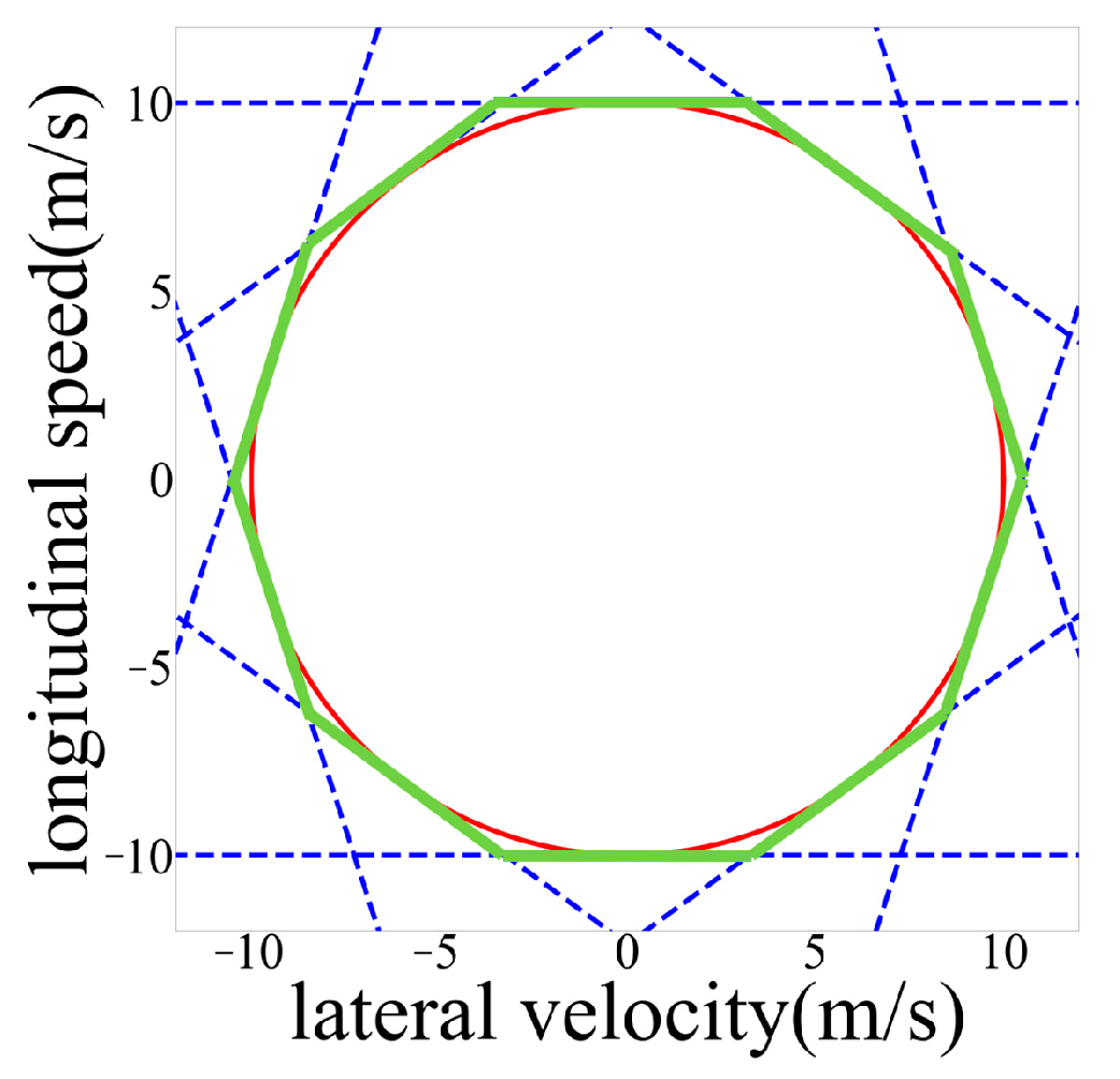
3.1.2. Velocity and Acceleration Constraints

In real scenarios, the speed and acceleration of UAVs and UGVs are affected by their own dynamic performance. In this work, we assume that the maximum speed is $v_{max}$ and the maximum acceleration is $a_{max}$. In the Cartesian coordinate system, the constraints of velocity and acceleration are described by circles with radii of maximum velocity and maximum acceleration, as shown in Figure 1. The equation of the circle is nonlinear, which needs to be linearized to embed it into the MILP model.

In this paper, the circle is fitted in the form of a circumscribed regular polygon. Due to the circumscribed nature of the polygon around the inscribed circle, there are still areas within the polygon that do not belong to the inscribed circle. These areas do not comply with the constraint. Hence, it is imperative to maximize the number of sides of the regular polygon to ensure comprehensive coverage of the entire inscribed circle. Taking the speed constraint as an example, a regular M-gon is circumscribed with the maximum-speed-limit circle, as shown in Figure 1. The red line is the circle surrounded by the maximum-velocity vector in the Cartesian coordinate system, the blue dotted line is the linear constraint, and the area within the green solid line is the range of the final linearization constraint. The slope of the side $m$ is

$$k=\tan \left(2\pi m/M\right),\hspace{1em}m\in \left[1,2,\dots ,M\right]$$

(4)

Then, the expression of each straight line can be obtained from the point-to-line distance formula and can be described as

$$v_x\sin \left(\frac{2\pi m}{M}\right)+v_y\cos \left(\frac{2\pi m}{M}\right)=v_{max}$$

(5)

Therefore, the constraints on the final velocity can be described as

$$\begin{array}{c}\forall p\in [1,2,\dots ,N_d+N_v],\forall t\in [1,2,\dots ,T],\forall m\in [1,2,\dots ,M]\\ v_x\sin \left(\frac{2\pi m}{M}\right)+v_y\cos \left(\frac{2\pi m}{M}\right)\le v_{max}\end{array}$$

(6)

Velocity constraints are similar to acceleration constraints, which are not discussed individually in this article.

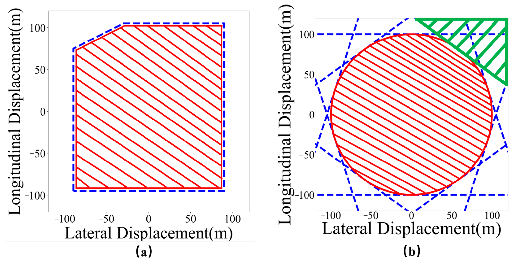
3.1.3. Obstacle Avoidance Constraints

During the movement of the UAVs and the UGVs, it is inevitable that they will encounter situations that cannot be passed. For UAVs, there are circular no-fly zones, irregular forests, etc. For UGVs, there are regular road boundaries, irregular lakes, etc. In order to reduce the number of constraints as much as possible and improve the calculation speed, irregular obstacle shapes are described by convex polygons or circles. As shown in Figure 2, the red areas are obstacles, the blue dotted lines are the linear constraints, and the green area is one of the feasible regions. Specifically, obstacles are described by convex polygons in Figure 2a, which are suitable for obstacles with clear boundaries and neat dividing lines. Obstacles are described by circles in Figure 2b, which are suitable for obstacles with complex shapes and fuzzy outlines. In this work, circles are used to represent obstacles.

Taking an obstacle with center coordinate $(x_{no},y_{no})$ and radius $R_{no}$ as an example, the avoidance constraints are

$$\begin{array}{c}\forall p\in [1,2,\dots ,N_d+N_v],\forall t\in [1,2,\dots ,T],\forall m\in [1,2,\dots ,M]\\ [x_p(t)-x_{no}]\sin \left(\frac{2\pi mW}{M}\right)+[y_p(t)-y_{no}]\cos \left(\frac{2\pi m}{M}\right)\ge R_{no}-(1-c_m^p)R_{inf}\end{array}$$

(7)

$$\begin{array}{c}\forall p\in [1,2,\dots ,N_d+N_v],\forall t\in [1,2,\dots ,T]\\ {\displaystyle \sum _{m=1}^M{c}_m^p}\ge 1\end{array}$$

(8)

where $R_{inf}$ is a constant with a value much larger than $R_{no}$, and $c_m^p$ is the binary decision variable of the obstacle avoidance constraint of the $p_{th}$ agent. When the value of $c_m^p$ is 0, Equation (8) is always established and does not act as a constraint. When the value of $c_m^p$ is 1, it indicates that the constraint condition is satisfied, and the position of the agents is restricted outside the constraint range. Equation (9) describes that $c_m^p$ requires at least one of the values to be 1, and its effect is shown in Figure 2b. As long as the agent is outside any edge of the polygon, the obstacle avoidance constraint can be satisfied.

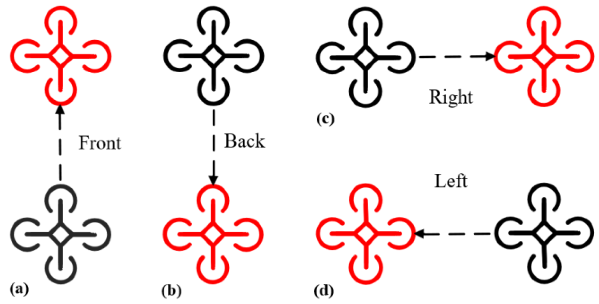
3.1.4. Dynamic Collision Constraints

Since all UAVs operate at the same altitude, and UGVs also operate on the ground at the same altitude, corresponding constraints must be taken to prevent individual collisions during operation. We take the collision avoidance of multiple drones as an example, as shown in Figure 3.

For a UAV, there are four motion directions, as shown in Figure 3, which are the front, back, right, and left. The dynamic anti-collision constraint of the agent can be described as the distance to any other UAV that maintains a safe threshold in each direction.

$$\begin{array}{c}\forall p,q\in [1,2,\dots ,N_d+N_v],\forall t\in [1,2,\dots ,T]\\ x_p(t)-x_q(t)\ge d_{safe}-(1-C_1^{pq})R_{inf}\\ x_q(t)-x_p(t)\ge d_{safe}-(1-C_2^{pq})R_{inf}\\ y_p(t)-y_q(t)\ge d_{safe}-(1-C_3^{pq})R_{inf}\\ y_q(t)-x_p(t)\ge d_{safe}-(1-C_4^{pq})R_{inf}\\ {\displaystyle \sum _{dir=1}^4{C}_{dir}^{pq}}=1\end{array}$$

(9)

Similar to the obstacle avoidance constraint, the distance between two individuals is limited by the value of the binary decision variable $C_{dir}^{pq}$ in Equation (9). When its value is 1, the collision avoidance constraint needs to be satisfied in this direction. At this time, the values of the other $C_{dir}^{pq}$ are all 0, which means that the collision avoidance constraints do not need to be satisfied in the other three directions.

3.1.5. Task Assignment Constraints

UAVs and UGVs differ in their specific functionalities and capabilities. UAVs, or unmanned aerial vehicles, are designed for airborne operations and are capable of tasks such as aerial reconnaissance, surveillance, and data collection. They leverage their aerial mobility to access difficult-to-reach areas and provide a comprehensive view from above.

On the other hand, UGVs, or unmanned ground vehicles, are ground-based platforms designed to operate on land. Their functionalities often include tasks such as ground-based surveillance, transportation of goods, and navigation in various terrains. UGVs are particularly well suited for tasks that require ground-level interactions and mobility.

While both UAVs and UGVs may share certain functionalities, such as surveillance, their differing platforms lead to variations in their capabilities. For instance, UAVs excel in tasks that demand aerial perspectives and swift mobility, whereas UGVs are more adept at ground-level operations and navigating diverse landscapes. Therefore, the task assignment of UAVs and UGVs can be treated as a multi-target detection task assignment problem for heterogeneous agents.

UAVs have a high-altitude view and can observe ground scenes from a bird’s eye view, which is more suitable for the exploration of vast flat areas. UGVs can observe the targets on the ground at closer range, which is more suitable for exhaustive searches of specified areas. However, drones are restricted by no-fly zones and cannot reach all areas. Flying in cities will also limit the minimum and maximum flight altitudes due to safety considerations. Therefore, in some cases, drones cannot complete all detection tasks. Similarly, UGVs also have problems such as being unable to cross lakes and dense forests.

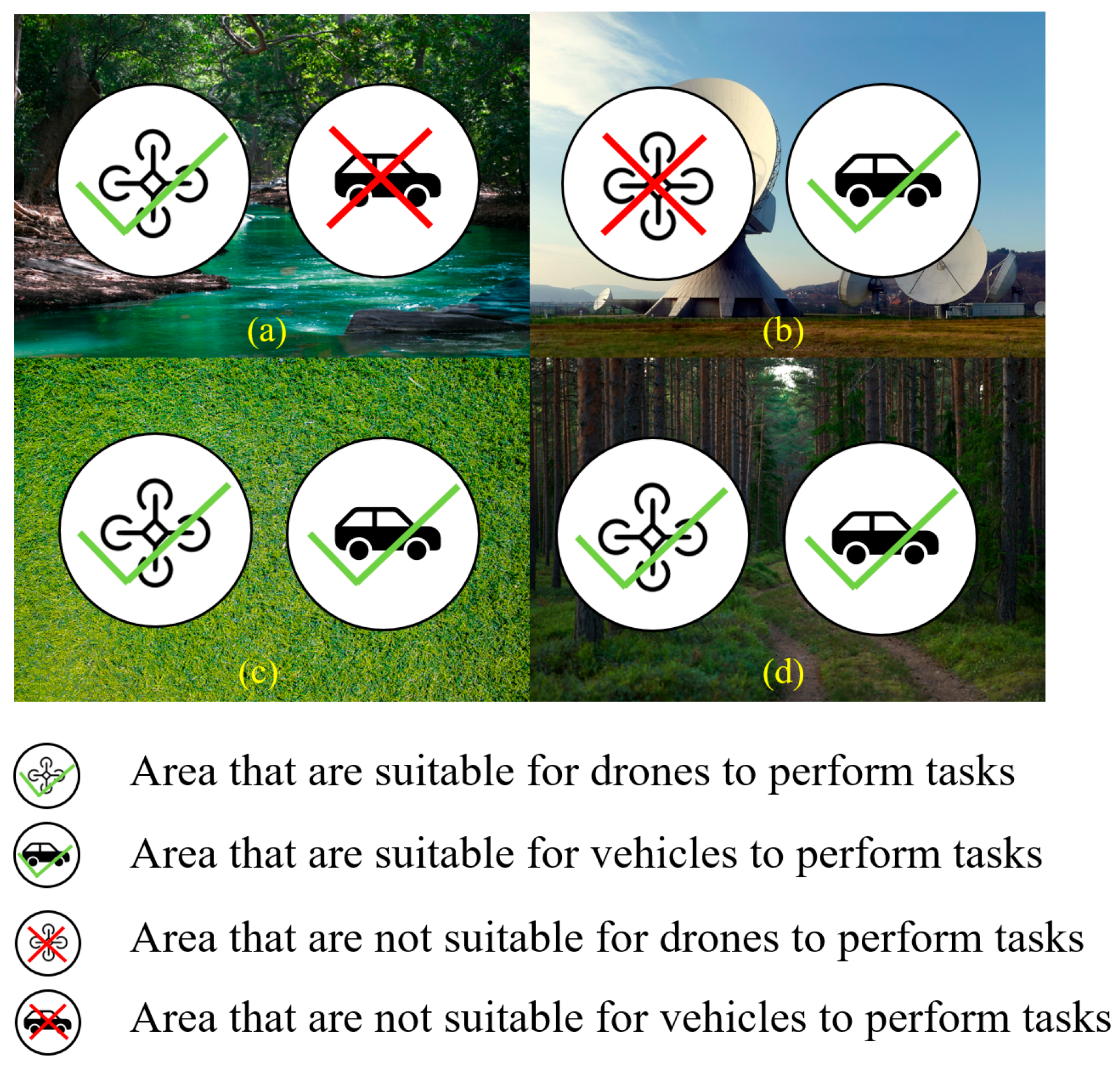
Therefore, to ensure that the arranged agents can complete the tasks sequentially, we need to fully consider which agent is suitable for the geographical environment and whether multiple agents are required in the allocation stage. The task assignment of the air–ground coordination problem can be divided into four types. As shown in Figure 4a, areas such as lakes, rivers, and dense forests cannot be passed by UGVs smoothly, in which it is more suitable to detect target points by UAVs. As shown in Figure 4b, drones cannot legally pass through military restricted areas and urban no-fly zones, and it is more suitable to detect these target points by UGVs. As shown in Figure 4c, in scenes such as open grasslands and roads with wild views, target points can be detected by both UAVs and UGVs. As shown in Figure 4d, in scenes like sparse forests and dense buildings with complex environments, target points cannot be clearly detected by UAVs or UGVs individually.

Therefore, the task assignment of the air–ground coordination problem can be divided into four cases:

Case1: target points suitable for UAVs.

Case2: target points suitable for UGVs.

Case3: target points suitable for both UGVs and UAVs.

Case4: target points that need to be detected by both UGVs and UAVs.

In this work, the binary decision variable $T_p^i(t)$ is used to indicate whether the $p_{th}$ agent needs to reach the target point at time step $t$. If it does, the value of $T_p^i(t)$ is 1. Otherwise, the value is 0. The complete equation can be described as

$$\begin{array}{c}\forall i\in [1,2,\dots ,N_{t1}]\\ {\displaystyle \sum _{p=1}^{N_d}{\displaystyle \sum _{t=1}^T{T}_p^i(t)=1}}\end{array}$$

(10)

$$\begin{array}{c}\forall i\in [1,2,\dots ,N_{t2}]\\ {\displaystyle \sum _{p=1}^{N_v}{\displaystyle \sum _{t=1}^T{T}_p^i(t)=1}}\end{array}$$

(11)

$$\begin{array}{c}\forall i\in [1,2,\dots ,N_{t3}]\\ {\displaystyle \sum _{p=1}^{N_v+N_d}{\displaystyle \sum _{t=1}^T{T}_p^i(t)=1}}\end{array}$$

(12)

$$\begin{array}{c}\forall i\in [1,2,\dots ,N_{t4}]\\ \left\{\begin{array}{l}{\displaystyle \sum _{p=1}^{N_d}{\displaystyle \sum _{t=1}^T{T}_p^i(t)=1}}\\ {\displaystyle \sum _{p=1}^{N_v}{\displaystyle \sum _{t=1}^T{T}_p^i(t)=1}}\end{array}\right.\end{array}$$

(13)

where Equation (10), Equation (11), Equation (12), and Equation (13) describe Case1, Case2, Case3, and Case4, respectively.

3.1.6. Task Completion Constraints

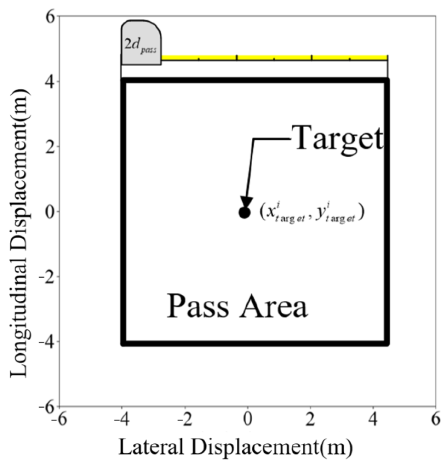
In the task allocation constraints, each task point is assigned for detection by the corresponding UAV or UGV, and the arrival time (number of time steps) is clearly specified. Therefore, it is necessary to construct the task completion constraint to ensure that the UAV or UGV reaches the target point (or is close enough to the target point) at the specified number of time steps. As shown in Figure 5, as long as the agent reaches target point $i$ with coordinates $\left(x_{\mathit{target}}^i,y_{\mathit{target}}^i\right)$, within the square with side length $2d_{pass}$ at the specified time step $t$, the agent can be considered to have completed the task.

The mathematical expression of task completion constraints can be described as

$$\begin{array}{c}\forall p\in [1,2,\dots ,N_d+N_v],\forall i\in [1,2,\dots ,N_t],\forall t\in [1,2,\dots ,T]\\ x_p(t)-x_{\mathit{target}}^i\le d_{pass}+(1-T_p^i(t))R_{inf}\\ x_{\mathit{target}}^i-x_p(t)\le d_{pass}+(1-T_p^i(t))R_{inf}\\ y_p(t)-y_{\mathit{target}}^i\le d_{pass}+(1-T_p^i(t))R_{inf}\\ y_{\mathit{target}}^i-y_p(t)\le d_{pass}+(1-T_p^i(t))R_{inf}\end{array}$$

(14)

3.2. Objective Function

The objective function of the air–ground collaborative multi-target detection task model established in this paper consists of four elements, which are the shortest time, the total time, the total energy consumption, and the smoothness of the trajectory.

3.2.1. The Shortest Time

The shortest time refers to the total time consumed when the last target point is detected, and the mathematical expression can be written as

$$\begin{array}{c}\forall p\in [1,2,\dots ,N_d+N_v],\forall i\in [1,2,\dots ,N_t],\forall t\in [1,2,\dots ,T]\\ t_{max}\ge t·T_p^i(t)\\ J_1=\min t_{max}\end{array}$$

(15)

where $t_{\max }$ represents the longest global time and $J_1$ is the optimization function. By comparing the constraint and the minimum objective function, the minimization time $t_{\max }$ is described in a linear manner.

3.2.2. The Total Time

The total time equals the summation of the time cost by each UAV and UGV to complete the task, which can be described as

$$\begin{array}{c}\forall i\in [1,2,\dots ,N_t],\forall t\in [1,2,\dots ,T]\\ t_{max}^p\ge t·T_p^i(t)\\ J_2=\min {\displaystyle \sum _{p=1}^{N_d+N_v}{t}_{max}^p}\end{array}$$

(16)

where $t_{max}^p$ represents the time for the $p_{th}$ agent for completion of all tasks. $J_2$ is the optimization function.

3.2.3. The Total Energy Consumption

Under the condition of constant speed, the energy consumption of the UGV is related to the running time, which can be obtained by the following derivation described in [26] for the UAV.

Assuming that the air velocity generated by a single propeller of the UAV is $v$, and the air mass is $m_{air}$, it can be inferred that the kinetic energy produced by the propeller without considering air friction is

$$E=\frac{1}{2}{m}_{air}{v}^2$$

(17)

The air quality $m_{air}$ can be expressed as

$$m_{air}=\pi r^{v}vt\rho$$

(18)

where $\rho$ is the air density at the current altitude and $r$ is the radius of the propeller. Therefore, for a six-rotor UAV, the energy consumption $P$ is

$$P=6\frac{dE}{dt}=3{\pi }^2{v}^3\rho$$

(19)

Equation (19) can also be rewritten as

$$P=Fv=mgv$$

(20)

where $m$ is the mass of the UAV and $g$ is the local gravitational acceleration. Combining Equations (19) and (20), we can obtain

$$P=\sqrt{\frac{{(mg)}^3}{2\pi r^2\rho }}$$

(21)

Therefore, for UAVs, the energy consumption in the hovering state is positively related to the time. Similarly, in the state of uniform motion, Equation (20) can be rewritten as

$$P=F_{1}v=\frac{mgv}{\cos \theta }$$

(22)

where $\theta$ is the angle between the axis of the drone and the vertical line. We can find that in the state of uniform motion, the energy consumption is only positively correlated with time.

Therefore, with constant speed, the total energy consumption target $J_3$ can be described as

$$J_3=\min {\displaystyle \sum _{p=1}^{N_d+N_v}{\displaystyle \sum _{t=1}^{T-1}\alpha \left[\frac{x_p(t+1)-x_p(t)}{v_{px}(t)}+\frac{y_p(t+1)-y_p(t)}{v_{py}(t)}\right]}}$$

(23)

where $\alpha$ is a proportional coefficient, which is used for the dimension conversion of energy consumption and time and can also be used to adjust the proportion of total energy consumption $v_{px}(t)$ and $v_{py}(t)$ representing the horizontal and vertical speeds of the $p_{th}$ agent at time step $t$, respectively.

3.2.4. The Smoothness of the Trajectory

In order to facilitate the tracking of trajectory points by UAVs and UGVs in real scenarios, the trajectory points generated by the proposed path planning algorithm should be as smooth as possible. In this work, we construct the constraint of the smoothness of the trajectory as

$$J_4=\min {\displaystyle \sum _{p=1}^{N_d+N_v}{\displaystyle \sum _{t=1}^{T-1}\beta \left[\frac{a_{px}(t+1)-a_{px}(t)+a_{py}(t+1)-a_{py}(t)}{\Delta t}\right]}}$$

(24)

where $\beta$ is a proportional coefficient, which is used for the dimension conversion of energy consumption and time and can also be used to adjust the proportion of trajectory smoothness loss in the objective function. $a_{px}(t)$ and $a_{py}(t)$ represent the lateral and vertical accelerations of the $p_{th}$ agent at time step $t$, respectively.

4. Optimal Solution Method of Mathematical Model

After establishing the mathematical model, it is necessary to design a corresponding solution method to solve the model to obtain a solution with appropriate accuracy. The model designed in this article can be solved by traditional optimization methods or heuristic algorithms, but the original algorithm still needs to be appropriately modified to ensure that the calculation can converge and speed up the calculation as much as possible.

4.1. Branch-and-Bound

The branch and bound (B&B) method was proposed by Land [27] in the 1960s to solve integer programming problems and then extended by [28] to solve MILP problems. The core idea of this method lies in branching, delimiting, and pruning.

Specifically, suppose a Mixed Integer Linear Programming problem $A$ to find the minimum solution, and suppose its corresponding linear programming problem $B$. Starting from solving problem $B$, if the optimal solution does not meet the integer condition of $A$, then the optimal objective function value $z$ must be the lower bound of the optimal objective function value $z^{\ast }$ of $A$, denoted as $\underset{¯}{z}$. Furthermore, the value of the objective function for any feasible solution of $A$ will be the upper bound of $z^{\ast }$, denoted as $\overline{z}$. The Branch-and-Bound method divides the feasible region into several sub-regions, and this process is called branching. After that, each sub-region will solve the new upper bound ${\overline{z}}_{new}$ and lower bound ${\underset{¯}{z}}_{new}$ as the boundary of the region, which is called delimitation. If the new lower bound ${\underset{¯}{z}}_{new}$ is greater than the known optimal solution $z_{\mathrm{now}}^{\ast }$, it means that the region has been searched and no further branching is required, and its subset may not be considered, which is called pruning. In short, the Branch-and-Bound method needs to gradually reduce $\overline{z}$ and increase $\underset{¯}{z}$ in the iterative process, and finally find $z^{\ast }$. The algorithm framework of B&B is shown in Algorithm 1.

Algorithm 1 Branch-and-Branch

Input: A mixed integer programming problem $A$, the upper bounds of the current solution $\overline{z}$, the lower bounds of the current solution $\underset{¯}{z}$, $B$ is the corresponding linear programming problem of $A$, $B^{\prime }$ is a branch of $B$

Output: The optimal solution $z^{\ast }$

1: while solution of $B$ is not empty do 2:  if $B^{\prime }$ is feasible then 3:     Let $z$ be optimal solution of $B^{\prime }$ 4:     if $z>\overline{z}$ then 5:       Cut the branch $B^{\prime }$ 6:    end if

7:     if $z$ satisfies integral solution of $A$ then 8:       if $z<\overline{z}$ then 9:         $\overline{z}=z$ 10:      end if 11:    else 12:       $\underset{¯}{z}=z$ 13:    end if 14:  end if 15: end while 16: return $\overline{z}$

4.2. Improved Genetic Algorithm and A* Algorithm

The Genetic Algorithm has a faster solution speed in task allocation and path planning, but in this paper, task planning and path planning have a strong coupling relationship, which makes it difficult for traditional Genetic Algorithms to effectively solve this type of problem by designing simple chromosomes and genetic operators. Therefore, in this paper, the Genetic Algorithm is used to assign tasks, the A* algorithm is used to obtain the path planning results, and the objective function value obtained as a whole is used as the fitness value of the Genetic Algorithm. The specific process is described in Algorithm 2.

Algorithm 2 Genetic Algorithm Process

1: Initialize the population 2: Coding chromosome 3: while the number of iterations is not reached do 4:   Calculate fitness 5:   Select operation 6:   Crossover operation 7:    if chromosomes need to be adjusted then 8:     Adjust operation 9:    end if 10:   Mutate operation 11:   Generate a new generation 12: end while

The population size $N_{per}$, selection probability, crossover probability, mutation probability, and maximum evolutionary algebra need to be determined for initialization of the population.

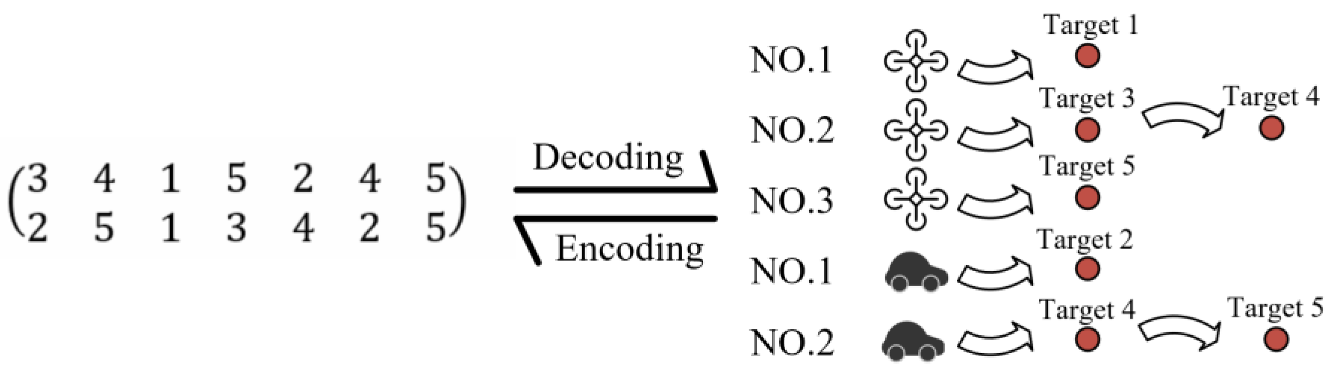
To encode the chromosome, we take the chromosome as a two-layer code. Among them, the first layer of the chromosome code represents the execution order of all target points, and the second layer represents the ID number of the agent required for detection of the corresponding target point. If the total number of target points is $N_t$, and the number of target points that need to be detected by both UAV and UGV is $N_{t4}$, then the length of the chromosome is $N_t+N_{t4}$. For instance, if there are three UAVs and two UGVs—a total of 5 target points, including 2 target points that need to be detected by both UAVs and UGVs and 3 target points that need to be detected by UAVs or UGVs—then the encoded chromosome can be described as in Figure 6.

From Figure 6, we know that UAV No. 1 performs the detection task of target point No. 1, UAV No. 2 performs the detection task of target point No. 3 and No. 4 in turn, UAV No. 3 performs the detection task of target point No. 5, UGV No. 1 performs the detection task of target point No. 2, and UGV No. 2 performs the detection task of target point No. 4 and No. 5 in turn. Chromosomes encoded by this method can meet the constraints of assignment of task points.

In this step, according to the target points that need to be detected by the corresponding agent after decoding the individual $i_{per}$, the planned path of each agent can be obtained through the A* algorithm. After that, the optimization solution calculated by the above objective function is the original fitness $J(i_{per})$. In order to facilitate the selection of population individuals later, the final fitness $Fitness(i_{per})$ is set as

$$Fitness(i_{per})=\frac{1}{J(i_{per})}$$

(25)

The magnitude of fitness implies the length of the path and, consequently, the resource consumption. A higher fitness value indicates a lower resource consumption.

The selection phase adopts elitism, that is, individuals with higher fitness are more likely to be retained in the genetic process. Therefore, the selection probability for an individual is

$$p(i_{per})=Fitness(i_{per})/{\displaystyle \sum _{i_{per}=1}^{N_{per}}Fitness(i_{per})}$$

(26)

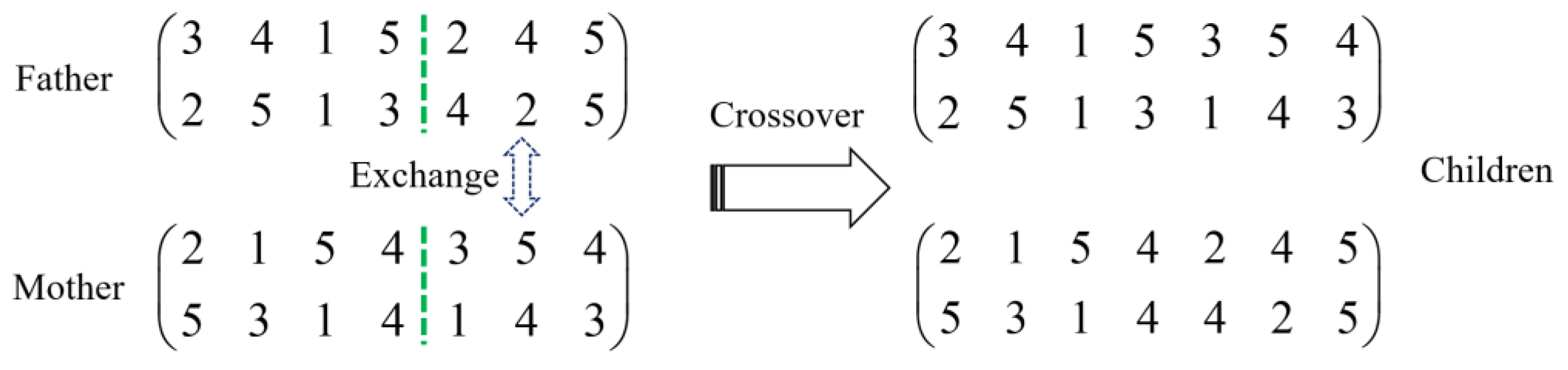
According to the crossover probability, we can select two chromosomes from the population, randomly determine the crossover position on the chromosome, and perform crossover operation on the gene codes. For example, after selecting two individuals to cross at the fifth position, the specific effect can be obtained as shown in Figure 7. The chromosome is divided into two parts by a green line, and the parent and mother generations cross over on the right half of the green line.

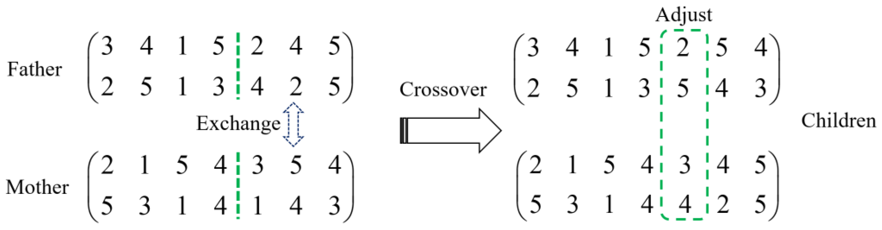
Unless the genes of the crossover position of the two individuals of the parent are identical, the offspring generated by this method will have the phenomenon of missing target points and repeated target points at the same time, and the number of missing target points will be the same as that of repeated target points. Therefore, a one-step adjustment operation is required to replace redundant task points with missing target points. After that, it is necessary to check whether the agent distribution of the offspring meets the requirements. The adjusted individual is shown in Figure 8, and the two offspring can meet the coding requirements and can further participate in the subsequent evolution.

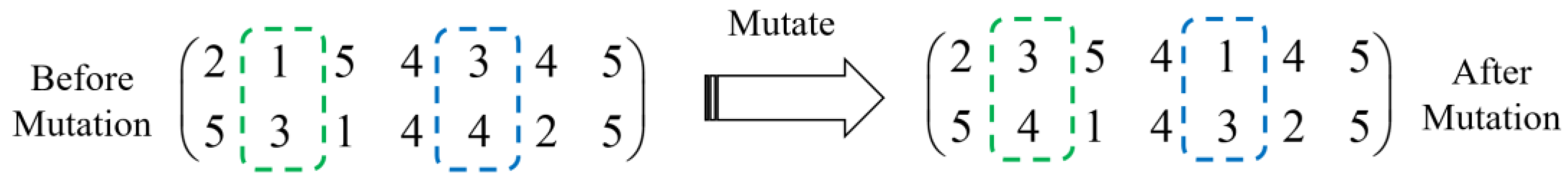
According to the mutation probability, the individual that needs to be mutated is randomly selected in the population, two mutation positions are also randomly selected from the chromosome of the individual, and the two mutation positions are exchanged. The specific implementation of the proposed method is shown in Figure 9. The genes in the green and blue boxes meet the model requirements through reasonable mutation.

The selected parent chromosomes and the offspring chromosomes generated after crossover and mutation operations are merged to form a new generation of populations.

The fitness value of the new population is calculated, and it is determined whether the contemporary optimal result satisfies the iteration termination condition. If not, we skip to step 4 to select a new generation and start a new generation of evolutionary iteration. If the maximum number of iterations has been reached, the Genetic Algorithm ends.

4.3. Branch-and-Bound with Improved Genetic Algorithm (IGA-B&B)

The hot start method for the B&B algorithm is commonly used to solve small-scale MILP problems. It requires pre-provision of a set of feasible solutions to limit the bounds. In this paper, we pre-provide a set of feasible solutions, which can be obtained by the proposed Improved Genetic Algorithm to limit the upper bound of the problem, thereby improving the efficiency of pruning and the speed of the overall operation.

The specific implementation involves initially disregarding the kinematic parameters of UAVs and UGVs, reducing the problem under study to a simplified single-agent path planning problem. An Improved Genetic Algorithm is then employed to find an initial solution. Since it is certain that this solution is not better than the optimal solution, it can serve as an upper bound for the B&B algorithm.

Furthermore, by initializing the B&B algorithm with the upper bound obtained, it effectively partitions the explored space, significantly enhancing the search speed and algorithm efficiency. The algorithm framework of this specific algorithm is shown in Algorithm 3.

Algorithm 3 Branch-and-Branch combined with Improved Genetic Algorithm

1: Employ Improved Genetic Algorithm to find initial solution $z_{iga}$ 2: Set $z_{iga}$ as the upper bound for $B$ 3: Initialize Branch-and-Bound algorithm with the upper bound $z_{iga}$ 4: while solution of $B$ is not empty do 5:   Select a branch $B^{\prime }$ from $B$ 6:   if $B^{\prime }$ is feasible then 7:      Let $z^{\prime }$ be optimal solution of $B^{\prime }$ 8:     if $z^{\prime }>z_{iga}$ then 9:      cut the branch $B^{\prime }$ 10:     else 11:      Update $z_{iga}\leftarrow z^{\prime }$ 12:     end if 13:   end if

14:     if $z_{iga}$ satisfies integral solution of $A$ then 15:      $z^{\ast }\leftarrow z_{iga}$ 16:      Break 17:     end if 18: end while 19: return $z^{\ast }$

5. Simulation Comparison and Experimental Verification

In order to increase the contrast and minimize the impact of environmental changes on the model, a grid map with the same environmental scene is used in our simulation test and the kinematic constraints are limited to the maximum speed and maximum acceleration. Each agent can only move in 8 directions. There are three UAVs and two UGVs, a total of eight mission points, two no-fly zones for UAVs, and two no-go zones for UGVs in the simulation maps.

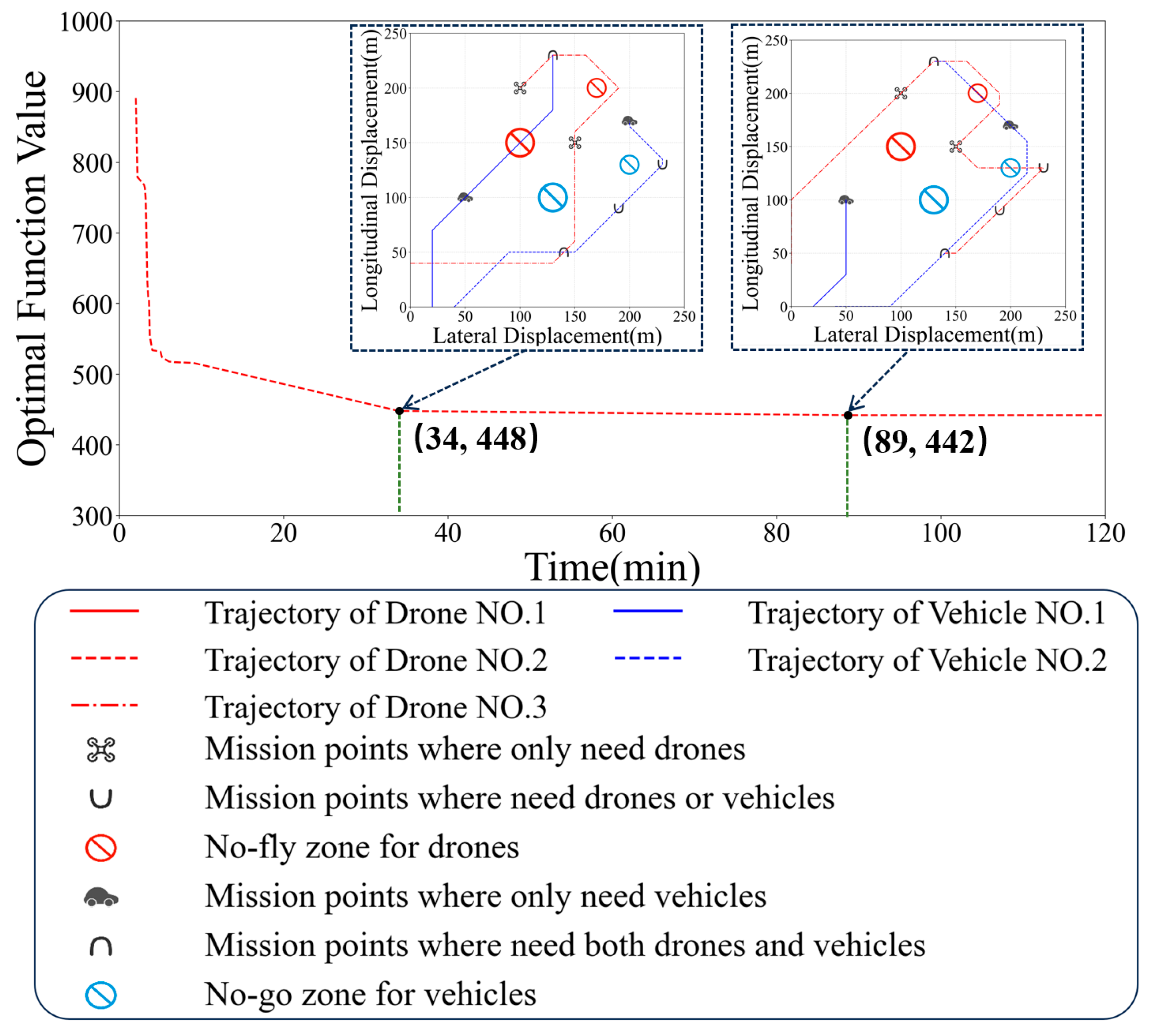
Although the Branch-and-Bound method has the ability to solve the global optimization problem, the excessive running time is unacceptable. It can be seen from the curve in Figure 10 that after 34 min, as the running time increases, the value of the objective function barely changes and the final generated trajectory hardly improves. Therefore, in the subsequent simulation experiments, the running time is set as 34 min.

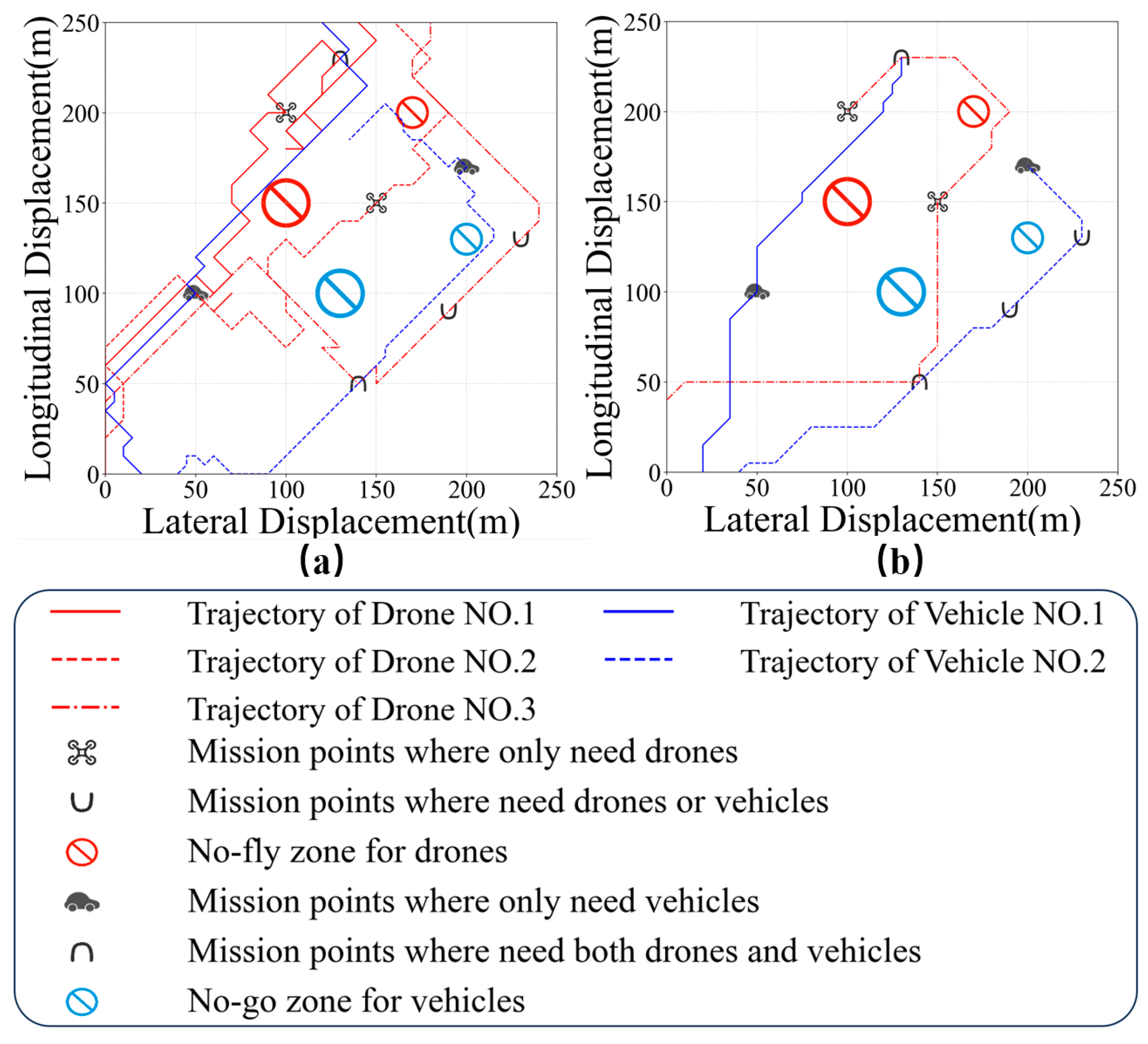
In the model with only the shortest time as the objective function, due to the lack of constraints on the running mileage, there are two bad results: one is that the agent with a task will not stop after completing the task; the other is the behavior of the agent without a task is not guided and constrained by the objective function, resulting in trajectory chaos, as shown in Figure 11a. These problems can be effectively solved after adding energy consumption constraints, as shown in Figure 11b.

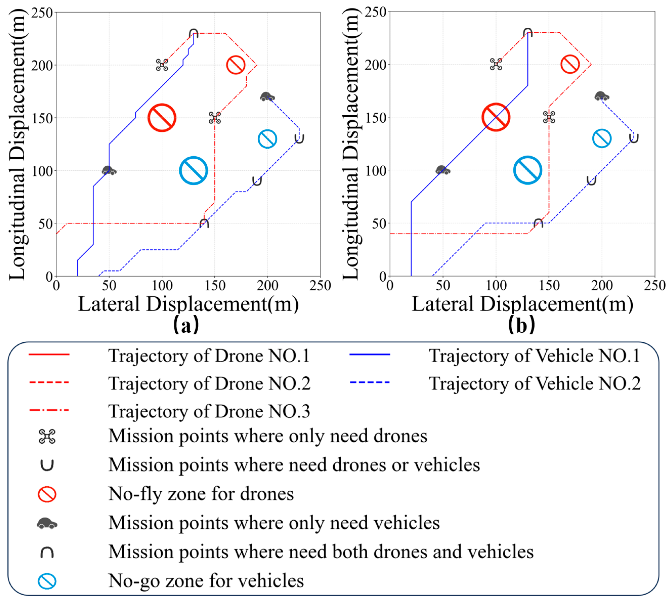
After adding the trajectory smoothness constraint to the objective function, compared with the model with only time and energy consumption constraints, the problem of continuous direction changes of each agent can be greatly improved, thereby reducing the difficulty of path following controlling and unnecessary energy consumption, as shown in Figure 12.

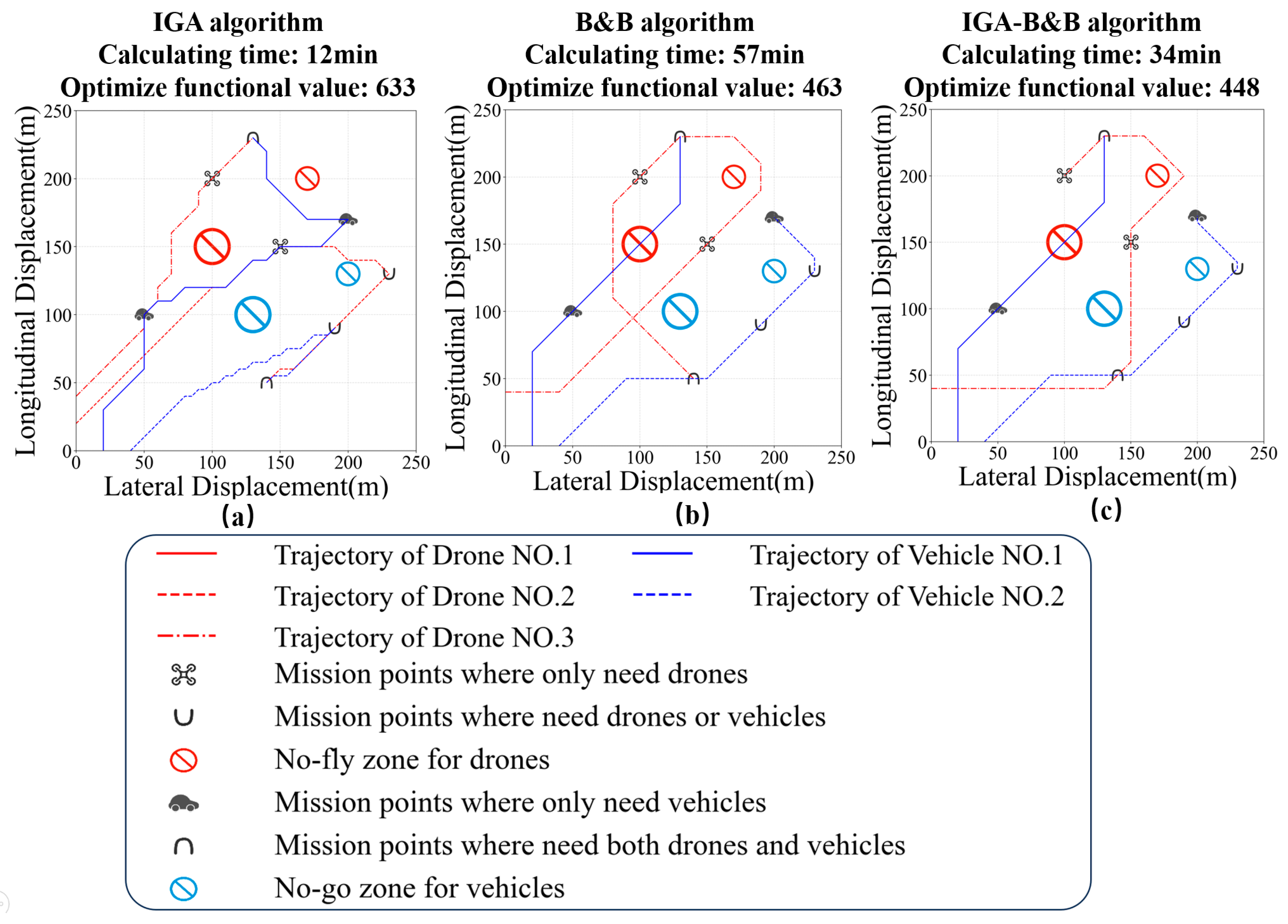
To verify the superiority of the proposed IGA-B&B algorithm, we compared simulation results by using several different objective-function-solving methods, as shown in Figure 13. From Figure 13a, we know that the Genetic Algorithm has a faster calculation time, but due to the lack of dynamic constraints of the A* algorithm, the final path is relatively discontinuous and the final optimal value of the objective function is lower. The final value of the objective function is 633 by using the Genetic Algorithm method and this value barely reduces with the increase in calculation time. Although the traditional B&B method can effectively obtain the optimal solution, the traversal search speed is slow and high computation memory is needed, resulting in slow running speed and even memory overflow, as shown in Figure 13b. The proposed IGA-B&B method can fully take advantage of the Genetic Algorithm and B&B methods, which means that the calculation time is effectively reduced by 30% and a relatively good allocation result can also be obtained, as shown in Figure 13c.

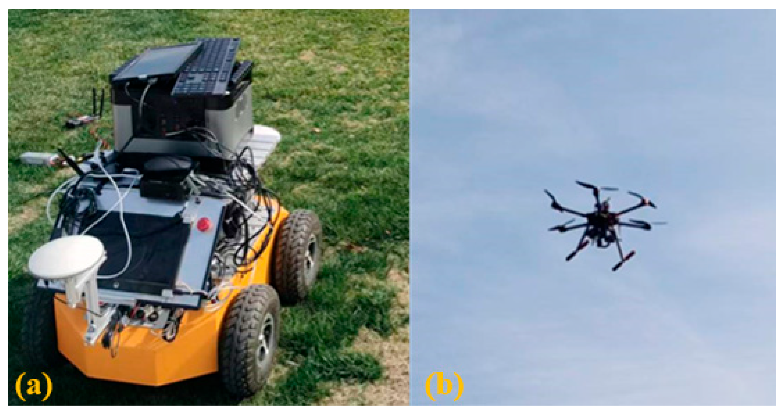
In order to verify the feasibility of the proposed model, experiments are carried out in the outdoor environment. The relevant testing equipment used in this work is shown in Figure 14.

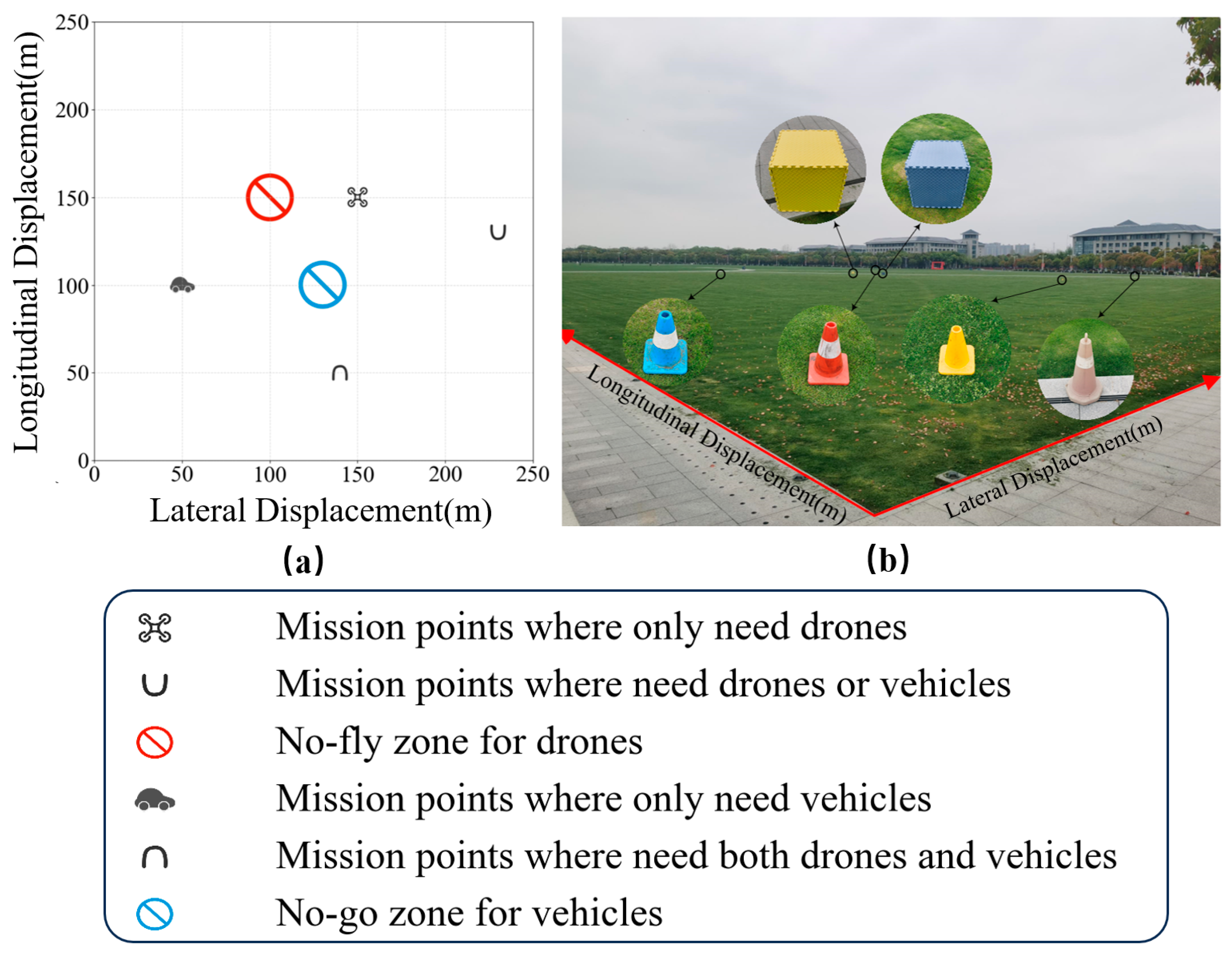
There are one UAV and one UGV, a total of four mission points, one simulated no-fly zone for UAVs, and one simulated no-go zone for UGVs in our experimental scene, which is located in a square area with a side length of 250 m in the Southeast University campus, as shown in Figure 15.

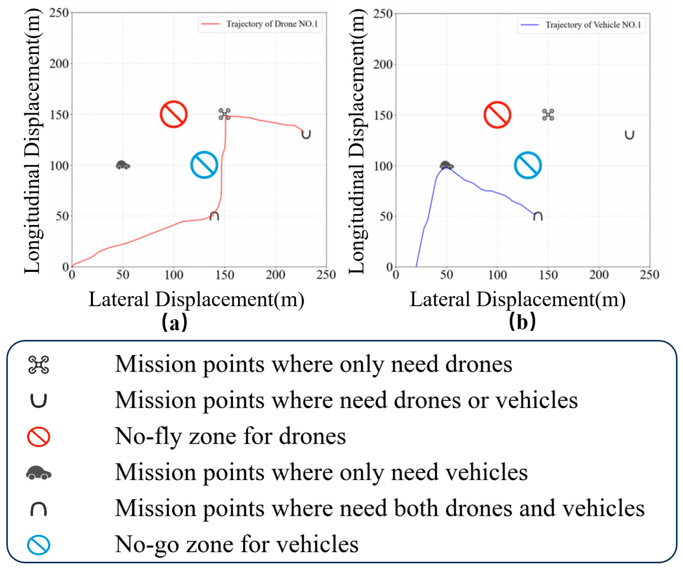
Using our proposed method, the target point detection tasks of UAVs and UGVs are assigned, and the optimal paths are also planned. Under the action of their respective path tracking controller, the UAVs and UGVs move along the planned paths. They are able to closely follow the planned trajectories and successfully complete tracking of all path points within 3 min. Their respective trajectories are shown in Figure 16a,b. It can be seen that UAVs and UGVs effectively reach the target points and successfully avoid their respective prohibited areas, further demonstrating the effectiveness and practicability of the proposed method.

6. Conclusions

In this paper, an air–ground collaborative multi-target detection task model based on Mixed Integer Linear Programming (MILP) is proposed. In this model, kinematic constraints of the UAVs and UGVs, dynamic collision avoidance constraints, task allocation constraints, and obstacle avoidance constraints are considered. In addition, an objective function with optimization directions of time consumption, energy consumption, and trajectory smoothness is established. To solve this objective function, a Branch-and-Bound method combined with the Improved Genetic Algorithm (IGA-B&B) is proposed and the optimal task assignment and optimal path of air–ground collaborative multi-target detection can be obtained. A simulation environment with multi-agents, multi-obstacles, and multi-task points is established. The simulation and experimental results show the effectiveness and feasibility of the proposed method.

In order to facilitate calculation and simplify the problem, many assumptions were set during our model construction process, which to some extent lost the authenticity of the model. For example, we ignore the energy loss caused by the ascent and descent of the drone. In addition, when facing extremely complex environmental conditions, such as scenes with a large number of UAVs and UGVs, and a significant number of target task points and no-go or no-fly zones, the proposed method may not be able to find a feasible solution within the specified time. Therefore, in order to further broaden the application range of the proposed model, we will focus on designing a novel objective-function-solving algorithm to achieve fast and approximate solutions in our following work.

References

- Jeong, J.; Tian, H.; Du, D. Trajectory-Based Data Forwarding Schemes for Vehicular Networks. ZTE Commun. 2014, 12, 17–25. [Google Scholar]
- Yang, J.; Ding, Z.; Wang, L. The Programming Model of Air-Ground Cooperative Patrol Between Multi-UAV and Police Car. IEEE Access. 2022, 9, 134503–134517. [Google Scholar] [CrossRef]
- Roberts, W.; Griendling, K.; Gray, A.; Mavris, D. Unmanned vehicle collaboration research environment for maritime search and rescue. In Proceedings of the 30th Congress of the International Council of the Aeronautical Sciences, Daejeon, Republic of Korea, 25–30 September 2016. [Google Scholar]
- Sowmya, N.; Costas, A.; Guy, B.; Regina, L. Use of UAV-Borne Spectrometer for Land Cover Classification. Drones 2018, 2, 16–30. [Google Scholar]
- Murray, C.C.; Chu, A.G. The flying sidekick traveling salesman problem: Optimization of drone-assisted parcel delivery. Transp. Res. Part C Emerg. Technol. 2015, 54, 86–109. [Google Scholar] [CrossRef]
- Bouman, P.; Agatz, N.; Schmidt, M. Dynamic programming approaches for the traveling salesman problem with drone. Networks 2018, 72, 528–542. [Google Scholar] [CrossRef]
- Raj, R.; Murray, C. The multiple flying sidekicks traveling salesman problem with variable drone speeds. Transp. Res. Part C Emerg. Technol. 2020, 120, 102813. [Google Scholar] [CrossRef]
- Dell’Amico, M.; Montemanni, R.; Novellani, S. Modeling the flying sidekick traveling salesman problem with multiple drones. Networks 2021, 78, 303–327. [Google Scholar] [CrossRef]
- El-Adle, A.M.; Ghoniem, A.; Haouari, M. Parcel delivery by vehicle and drone. J. Oper. Res. Soc. 2019, 72, 398–416. [Google Scholar] [CrossRef]
- Wang, Z.; Sheu, J.B. Vehicle routing problem with drones. Transp. Res. Part B Methodol. 2019, 122, 350–364. [Google Scholar] [CrossRef]
- Huawei, M.; Kai, M.; Jun, G. Research on Vehicle Routing Problem with Drones Considering Multi-Delivery. Comput. Eng. 2022, 48, 299–305. [Google Scholar]
- Schermer, D.; Moeini, M.; Wendt, O. A matheuristic for the vehicle routing problem with drones and its variants. Transp. Res. Part C Emerg. Technol. 2019, 106, 166–204. [Google Scholar] [CrossRef]
- Gu, R.; Poon, M.; Luo, Z.; Liu, Y.; Liu, Z. A hierarchical solution evaluation method and a hybrid algorithm for the vehicle routing problem with drones and multiple visits. Transp. Res. Part C Emerg. Technol. 2022, 144, 103733. [Google Scholar] [CrossRef]
- Tian, X.T.; Xi, Q.B. Real Time Path Planning of UAVs Using MILP. Comput. Simul. 2009, 26, 72–75. [Google Scholar]
- Lv, Y.; Wan, X.; Shi, Y. Aircraft Collision Avoidance Trajectory Planning Based on MILP. Flight Dyn. 2005, 23, 81–84. [Google Scholar]
- Li, D.D.; Sun, X.X.; Sun, B.; Zhang, Y. Mission planning for UAVs based on MILP. Flight Dyn. 2010, 28, 88–91. [Google Scholar]
- Hu, Z.F.; Chen, Y.; Zheng, X.J.; Wu, H.Y. Cooperative patrol path planning method for air-ground heterogeneous robot system. Control Theory Appl. 2022, 39, 48–58. [Google Scholar]
- Wu, X.; Yin, Y.; Xu, L.; Wu, X.; Meng, F.; Zhen, R. Multi-UAV Task Allocation Based on Improved Genetic Algorithm. Mod. Electron. Tech. 2023, 46, 139–146. [Google Scholar] [CrossRef]
- Kim, M.H.; Baik, H.; Lee, S. Response Threshold Model Based UAV Search Planning and Task Allocation. J. Intell. Robot. Syst. 2014, 75, 625–640. [Google Scholar] [CrossRef]
- Zhang, M.Y.; Wang, M.Y.; Wang, X.D.; Song, X. Cooperative Real-Time Task Assignment of UAV Group Based on Improved Contract Net. Aero Weapon. 2019, 26, 38–46. [Google Scholar]
- Yan, F.; Zhu, X.P.; Zhou, Z.; Tang, Y. Real-time task allocation for a heterogeneous multi-UAV simul-taneous attack. Sci. Sin. Inf. 2019, 49, 555–569. [Google Scholar] [CrossRef]
- Chen, Y.; Chen, M.; Chen, Z.; Cheng, L.; Yang, Y.; Li, H. Delivery path planning of heterogeneous robot system under road network constraints. Comput. Electr. Eng. 2021, 92, 107197. [Google Scholar] [CrossRef]
- Wang, X.; Liu, Z.; Liu, J. Mobile Robot Path Planning Based on an Improved A* Algorithm. Robot 2018, 40, 903–910. [Google Scholar]
- Challita, U.; Saad, W.; Bettstetter, C. Interference Management for Cellular-Connected UAVs: A Deep Reinforcement Learning Approach. IEEE Trans. Wirel. Commun. 2019, 18, 2125–2140. [Google Scholar] [CrossRef]
- Liu, W.; Wang, Y. Path Planning of Multi-UAV Cooperative Search for Multiple Targets. Electron. Opt. Control 2019, 26, 35–38. [Google Scholar]
- Abeywickrama, H.V.; Jayawickrama, B.A.; He, Y.; Dutkiewicz, E. Comprehensive Energy Consumption Model for Unmanned Aerial Vehicles, Based on Empirical Studies of Battery Performance. IEEE Access 2018, 6, 58383–58394. [Google Scholar] [CrossRef]
- Land, A.H.; Doig, A.G. An automatic method for solving discrete programming. Econometrica 1960, 28, 497–520. [Google Scholar] [CrossRef]
- Dakin, R.J. A tree-search algorithm for mixed integer programming problems. Comput. J. 1965, 8, 250–255. [Google Scholar] [CrossRef]
Figure 1.
Maximum speed limit circle and linearization.
Figure 2.
Polygonal and circular descriptions of complex obstacles: (a) polygonal description; (b) circular description.
Figure 3.
The four orientations of the agent in the anti-collision constraint: (a) front, (b) rear, (c) right, (d) left.
Figure 4.
Four different example scenarios: (a) scene suitable for UAV; (b) scene suitable for UGVs; (c) scene suitable for both UGVs and UAVs; (d) scene that needs to be detected by both UGVs and UAVs.
Figure 5.
Schematic diagram of the task completion constraints of the target point.
Figure 6.
Description after chromosome encoding and meaning after decoding.
Figure 7.
Schematic diagram of chromosome crossover operation.
Figure 8.
Schematic diagram of chromosome crossover-adjustment operation.
Figure 9.
Schematic diagram of chromosome mutation operation.
Figure 10.
The effect of iteration time on the results of Branch-and-Bound method.
Figure 11.
The results of optimization with or without energy consumption constraints: (a) with only time constraint; (b) with time and energy consumption constraints.
Figure 12.
Optimization results with and without trajectory smoothness: (a) with time and energy consumption constraints; (b) with optimized time, energy consumption, and trajectory smoothness constraints.
Figure 13.
Comparison of several optimization methods: (a) Genetic Algorithm; (b) B&B; (c) IGA-B&B.
Figure 14.
Equipment used during the experimental test: (a) UGV; (b) UAV.
Figure 15.
The experimental scene: (a) schematic diagram; (b) side view of the experimental scene.
Figure 16.
Trajectories of UAVs and UGVs: (a) trajectory of UAVs; (b) trajectory of UGVs.