Image Encryption Using Chebyshev Map and Rotation Equation

Abstract

We propose a novel image encryption algorithm based on two pseudorandom bit generators: Chebyshev map based and rotation equation based. The first is used for permutation, and the second one for substitution operations. Detailed security analysis has been provided on the novel image encryption algorithm using visual testing, key space evaluation, histogram analysis, information entropy calculation, correlation coefficient analysis, differential analysis, key sensitivity test, and computational and complexity analysis. Based on the theoretical and empirical results the novel image encryption scheme demonstrates an excellent level of security.

1. Introduction

Over the past twenty years, the nonlinear chaotic systems have been ordinarily used in digital data encryption and transmission. In the imaginative work [1] of J. Fridrich is shown the good potential of the dynamical chaotic maps in symmetric image encryption. The paper highlights how to adapt nonlinear Baker map, Cat map and Standard map on a torus or on a rectangle in order of block encryption schemes.

An improved stochastic middle multi-bits quantification scheme based on Chebyshev map is proposed in [2]. Novel image encryption scheme with Chebyshev map based diffusion operations is presented in [3]. A novel design method of key stream by chaotic Chebyshev function is proposed in [4]. In [5], a secure Diffie-Hellman key agreement protocol based on Chebyshev chaotic map is presented.

In [6], a chaotic cipher is proposed to encrypt color images through position permutation part and Logistic map based on substitution. By using Chebyshev map and Arnold map, a bit-level permutation image encryption algorithm is proposed [7].

In [8], based on the Lorenz attractor and perceptron algorithm, a chaotic image encryption system is proposed. an image encryption scheme using dynamic sequences generated by multiple chaotic systems is presented in [9]. In [10], a bit-level permutation and Chen chaotic system are proposed to encrypt color images.

A chaos based image encryption scheme is proposed in this article. The novel algorithm is based on a simple multiple round substitution-permutation model. It is Chebyshev map based on permutation and rotation function based on substitution with motivation to maintain the high quality of the encrypted images. The novelty of our approach lies in the combination of two cryptographically strong pseudorandom generators.

In Section 2, we propose novel pseudo-random bit generator (PRBG) based on rotation function. In Section 2.2 in order to measure randomness of the bit sequence generated by the pseudo-random scheme, we use NIST, DIEHARD and ENT statistical packages. Section 4 presents the novel image encryption algorithm, and extended security cryptanalysis is given. Finally, the last section concludes the paper.

2. Pseudo-Random Bit Generator Based on the Rotation Equations

2.1. Proposed Pseudorandom Scheme

In this section, one real number of rotation formula is preprocessed to a binary pseudo-random sequence.

We are using rotation equations of the form [11,12]

$$\begin{array}{l}{x}_{t+1}=-a-(x_t-a)\cos \theta +y_t\sin \theta /r_t\\ y_{t+1}=-x_t{r}_t\sin \theta -y_t\cos \theta \\ r_t=\sqrt{0.5(x_t^2+\sqrt{x_t^4+4y_t^2}),}\end{array}$$

(1)

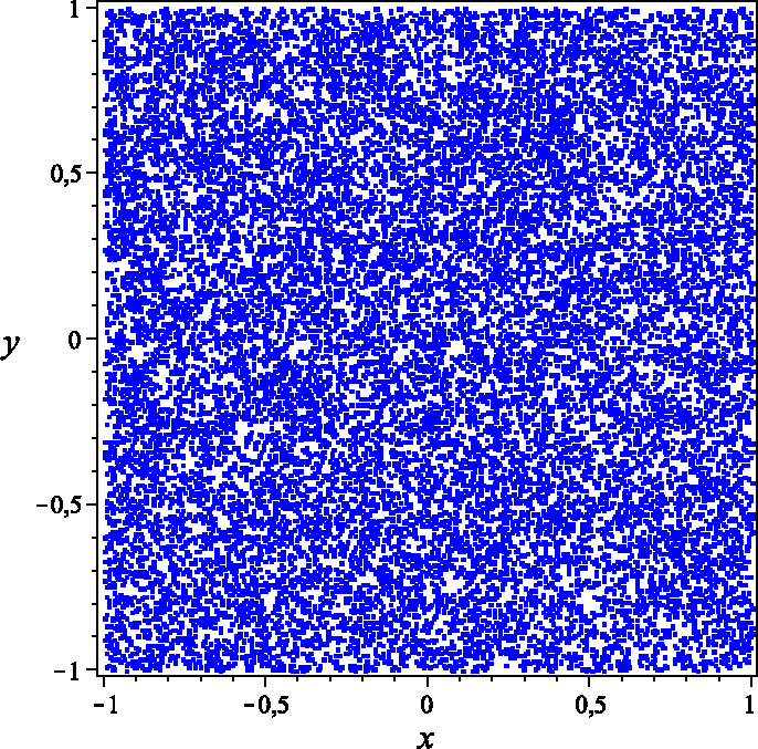
where the parameters are θ = 2 and a = 2.8. The rotation Equation (1) with initial conditions x₀ = 0.5, y₀ = 1.0 is graphed in Figure 1. This figure visually shows random-like positions of the points in the set.

The novel pseudorandom bit generation scheme consists of the following steps:

• Step 1: The initial values x₀ and y₀ from Equation (1) are determined.
• Step 2: The rotation equation, Equation (1), is iterated for L₀ times, where L₀ is a constant.
• Step 3: The iteration of the Equation (1) continues, and as a result, two decimal fractions x_i and y_i are generated.
• Step 4: The number y_i is post-processed as follows:

  $$s_i=mod(abs(integer(y_i\times {10}^5),2),$$

  (2)

  where mod(x, y) returns the reminder after division, abs(x) returns the absolute value of x, and integer(x) returns the integer part of x, truncating the value at the decimal point.
  The output bit s_i is obtained.
• Step 5: Return to Step 3 until pseudo-random bit stream limit is reached.

The rotation equations based pseudo-random bit scheme is implemented softwarely in C++ programming language, using the following initial values: x₀ = 0.2343214592, y₀ = −0.742190593, and L₀ = 140.

2.2. Statistical Test Analysis of the Pseudorandom Bit Generator Based on Rotation Equations

In order to measure randomness of the rotation equation based pseudo-random bit generator, we used NIST [13], DIEHARD [14], and ENT [15] statistical test suites.

Using the novel pseudo-random bit generator were produced 1000 sequences of 1,000,000 bits. The results from all tests are given in

Table 1. NIST test suite results.

NIST Statistical Test	Proposed PRBG
	p-Value	Pass Rate
Frequency (monobit)	0.450297	989/1000
Block-frequency	0.839507	987/1000
Cumulative sums (Forward)	0.032489	988/1000
Cumulative sums (Reverse)	0.668321	987/1000
Runs	0.224821	989/1000
Longest run of Ones	0.713641	990/1000
Rank	0.457825	991/1000
FFT	0.595549	988/1000
Non-overlapping templates	0.514662	990/1000
Overlapping templates	0.035174	985/1000
Universal	0.141256	988/1000
Approximate entropy	0.307077	989/1000
Random-excursions	0.693410	613/619
Random-excursions Variant	0.557718	613/619
Serial 1	0.576961	988/1000
Serial 2	0.221317	989/1000
Linear complexity	0.459717	987/1000

.

The entire NIST test is passed successfully: all the p − values are distributed uniformly in the 10 subintervals and the pass rate is also in acceptable range.

The minimum pass rate for each statistical test with the exception of the random-excursion (variant) test is approximately 980 for a sample size of 1000 zero-one sequences. The minimum pass rate for the random excursion (variant) test is approximately 605 for a sample size of 619 binary sequences for Rotation equations based pseudorandom bit generator. The proposed scheme possesses random-like properties.

For the DIEHARD tests, we generated a file with 80 million bits from the proposed pseudorandom bit generator. The results are placed in

Table 2. DIEHARD statistical test results.

DIEHARD, Statistical Test	Proposed PRBG, p-Value
Birthday spacings	0.339750
Overlapping 5-permutation	0.215056
Binary rank (31 × 31)	0.662314
Binary rank (32 × 32)	0.429881
Binary rank (6 × 8)	0.517681
Bitstream	0.448843
OPSO	0.542452
OQSO	0.491857
DNA	0.481574
Stream count-the-ones	0.983115
Byte count-the-ones	0.551900
Parking lot	0.551864
Minimum distance	0.447679
3D spheres	0.549807
Squeeze	0.265792
Overlapping sums	0.443169
Runs up	0.848733
Runs down	0.447462
Craps	0.295968

. All P-values are in acceptable range of [0, 1).

We tested the output of a string of 125,000,000 bytes of the proposed Rotation equations based pseudorandom bit generation scheme. The results are summarized in

Table 3. ENT statistical test results.

ENT, Statistical Test	Proposed PRBG, Results
Entropy Optimum compression	7.999998 bits per byte OC would reduce the size of this 125,000,000 byte file by 0%.
χ2 distribution	For 125,000,000 samples is 271.19, and randomly would exceed this value 23.21% of the time.
Arithmetic mean value	127.4982 (127.5 = random)
Monte Carlo π estim.	3.141377330 (error 0.01%)
Serial correl. coeff.	0.000001 (totally uncorrelated = 0.0)

. The proposed pseudorandom bit generator passed all the tests of ENT.

3. Pseudo-Random Bit Generator Based on the Chebyshev Map

In this section we will describe the Chebyshev map [16,17] based pseudorandom bit generator proposed in [18].

In [19], a pseudorandom bit stream is generated by comparing the outputs of two Chebyshev maps. In [20], the real numbers of two Chebyshev polynomials are post-processed and combined with a simple threshold function to a binary pseudorandom stream. The described scheme modify the generators in [19] and [20] by simple avoiding the threshold functions and speed up the bit extracting process with increasing the number of chaotic maps. The scheme is based on the following four Chebyshev maps:

$$\begin{array}{l}{T}_{n_1}(x_1)=2x_1{T}_{n_1-1}(x_1)-T_{n_1-2}(x_1)\\ T_{n_2}(x_2)=2x_2{T}_{n_2-1}(x_2)-T_{n_2-2}(x_2)\\ T_{n_3}(x_3)=2x_3{T}_{n_3-1}(x_3)-T_{n_3-2}(x_3)\\ T_{n_4}(x_4)=2x_4{T}_{n_4-1}(x_4)-T_{n_4-2}(x_4),\end{array}$$

(3)

where T₁(x₁), T₁(x₂), T₁(x₃), and T₁(x₄) are the initial values. The modified algorithm consists of the following steps:

• Step 1: The initial values T₁(x₁), T₁(x₂), T₁(x₃), and T₁(x₄) of the four Chebyshev maps from Equation (3) are determined.
• Step 2: The four Chebyshev maps from Equation (3) are iterated for K, L, M and N times, respectively, to avoid the harmful effects of transitional procedures.
• Step 3: The iteration of the Equation (3) continues, and as a result, four real fractions T_i(x₁), T_j(x₂), T_k(x₃), and T_l(x₄), are generated and post-processed as follows:

  $$\begin{array}{l}{s}_{m_1}=mod(intger(abs(T_i(x_1)\times {10}^{15})),2)\\ s_{m_2}=mod(intger(abs(T_j(x_2)\times {10}^{15})),2)\\ s_{m_3}=mod(intger(abs(T_k(x_3)\times {10}^{15})),2)\\ s_{m_4}=mod(intger(abs(T_l(x_4)\times {10}^{15})),2),\end{array}$$

  (4)

  where abs(x) returns the absolute value of x, integer(x) returns the integer part of x, truncating the value at the decimal point, and mod(x, y) returns the reminder after division. The four output bits $s_{m_1}$, $s_{m_2}$, $s_{m_3}$, and $s_{m_4}$ are obtained.
• Step 4: Return to Step 3 until the bit stream limit is reached.

The algorithm has good statistical properties measured by NIST, DIEHARD and ENT test packages.

4. Image Encryption Algorithm Based on Chebyshev Map and Rotation Equation

Here we describe an image encryption algorithm based on the proposed rotation equation based pseudo-random bit generator, Section 2, and Chebyshev map based pseudorandom bit generator [18]. We also present security analysis of the encrypted images.

4.1. Encryption Algorithm

The novel image encryption algorithm is a simple modification of the substitution-permutation scheme [1]. Here every single pixel encryption is based on pixel shuffling and pixel substitution, and on multiple overall rounds.

We consider plain images of n × n size. The binary length of n is n₀. The encryption process is divided in two parts. In the first part we generate buffer image B of n × n size by relocating the pixels of the plain image P by Chebyshev map based PRBG. In the second part we generate ciphered image C of n × n size by transforming the buffer pixel values by rotation equation based PRBG. The image encryption begins, with an empty buffer image. The entire encryption process is given below:

• Step 1: The Chebyshev map based PRBG is iterated six times to produce 24 bits. These bits constitute a binary number b_j.
• Step 2: The j^th column-vector is circularly shifted for mod (b_j) times.
• Step 3: Repeating Steps 1–2 until all of the columns, j = 1 … n, are processed, and the buffered image B is produced.
• Step 4: The rotation equation based PRBG is iterated to produce n × n × 8 bits for a monochrome image or n × n × 24 bits for a color image.
• Step 5: Do XOR operation between the pseudo-random bit sequence and all of the buffer pixels in the buffered image to produce the encrypted image C′.
• Step 6: Repeating Steps 1–5 for T ≥ 1 times, until encrypted image C is produced.

4.2. Security Analysis

The proposed image encryption algorithm is implemented in C++ programming language. All statistical results presented have been taken by T = 1.

Twenty eight 8-bit monochrome images and sixteen 24-bit color images have been encrypted for the statistical analysis. The test images are selected from the Miscellaneous volume of USC-SIPI image database. It is available and maintained by the University of Southern California Signal and Image Processing Institute ( http://sipi.usc.edu/database/). The color image names are from 4.1.01 to 4.1.08, size 256 × 256 pixels, from 4.2.01 to 4.2.07, size 512 × 512 pixels, and House, size 512 × 512 pixels. The monochrome images are from 5.1.09 to 5.1.14, size 256 × 256 pixels, from 5.2.08 to 5.2.10, size 512 × 512 pixels, 5.3.01 and 5.3.02, size 1024 × 1024 pixels, from 7.1.01 to 7.1.10, 7.2.01, size 512 × 512 pixels, and Boat, Elaine, Gray21, Numbers, Ruler, size 512 × 512 pixels, and Testpat, size 1024 × 1024 pixels.

4.2.1. Key Space Analysis

The set of all initial numbers compose the key space. The key space of the novel image encryption scheme has six secret key values x₀ = 0.2343214591, y₀ = −0.742190593, T₁(x₁) = 0.702938119500914, T₁(x₂) = −0.3001928364928377, T₁(x₃) = 0.1385946382912478, and T₁(x₄) = −0.2871955600387584, fixed as key K1. As stated in IEEE floating-point standard [21], the computational precision of the 64-bit double-precision number is about 10⁻¹⁵. The key space of the novel scheme is (10¹⁵)⁶ = 10⁹⁰ ≈ 2²⁹⁸. Furthermore, the initial iteration numbers K, L, M and N can also be used as a part of the key size.

Compared with similar image encryption algorithms [22–27], and [28] the proposed one has enough key space size,

Table 4. Keyspace comparisons.

Encryption Algorithm	Key Space
Proposed scheme	2298
Reference [22]	2197
Reference [23]	2292
Reference [24]	2149
Reference [25]	2256
Reference [26]	297
Reference [27]	2400
Reference [28]	2140

. The larger parameter space is based on the proposed combination of two different pseudorandom bit generators.

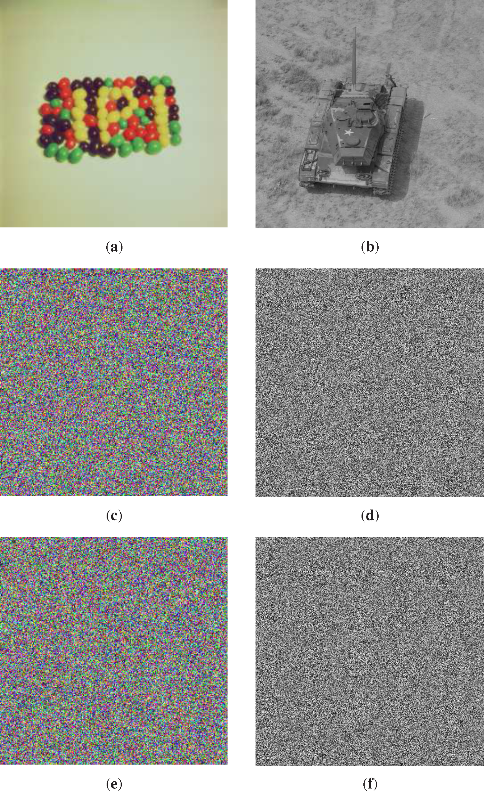
4.2.2. Visual Testing

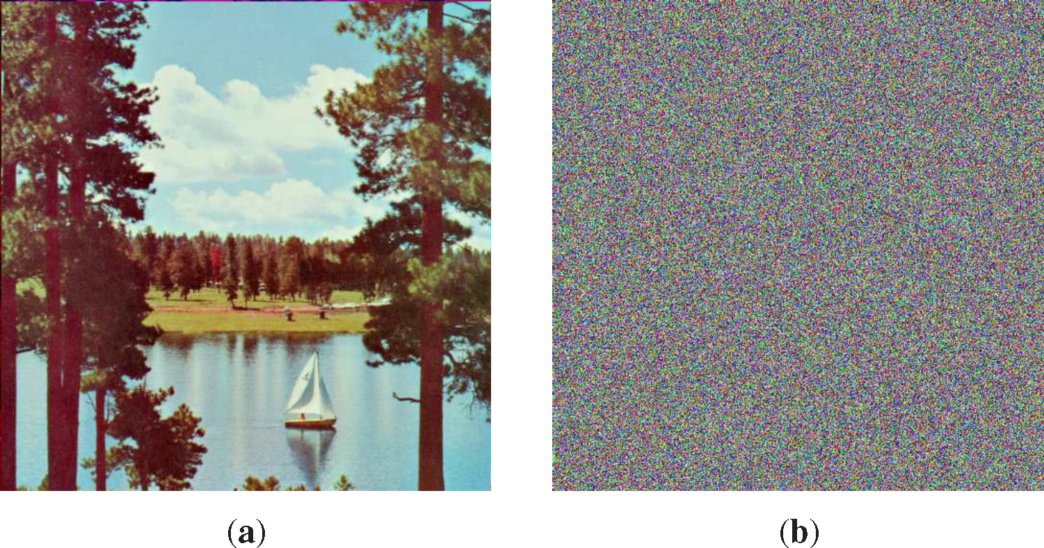
The novel image encryption scheme is tested by using visual review. The inspection does not detect analogy between plain images and their corresponding encrypted images. As an example, Figure 2 shows the image 4.2.06 Sailboat on lake, Figure 2a, and its encrypted version, Figure 2b. The encrypted image doesn’t keep any segmented color clusters and source figures.

4.2.3. Histogram Analysis

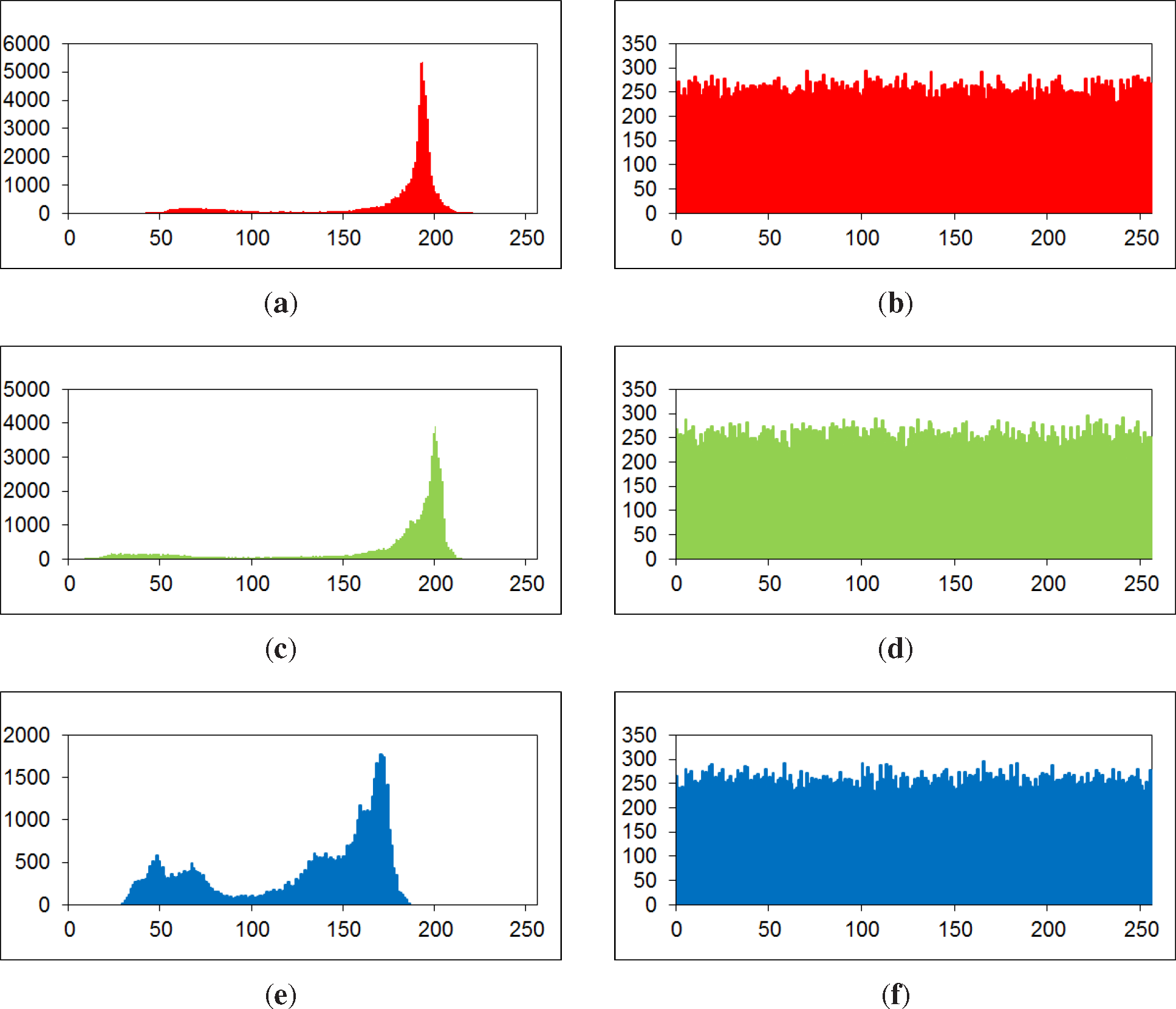
Histogram analysis of three channels (red, green, and blue) of the plain and encrypted images is given. Figure 3 shows the histograms of the 256 × 256 plain 4.1.08 Jelly beans and encrypted 4.1.08 Jelly beans. It is observed that the histograms of the encrypted image are significantly different from that of the plain image.

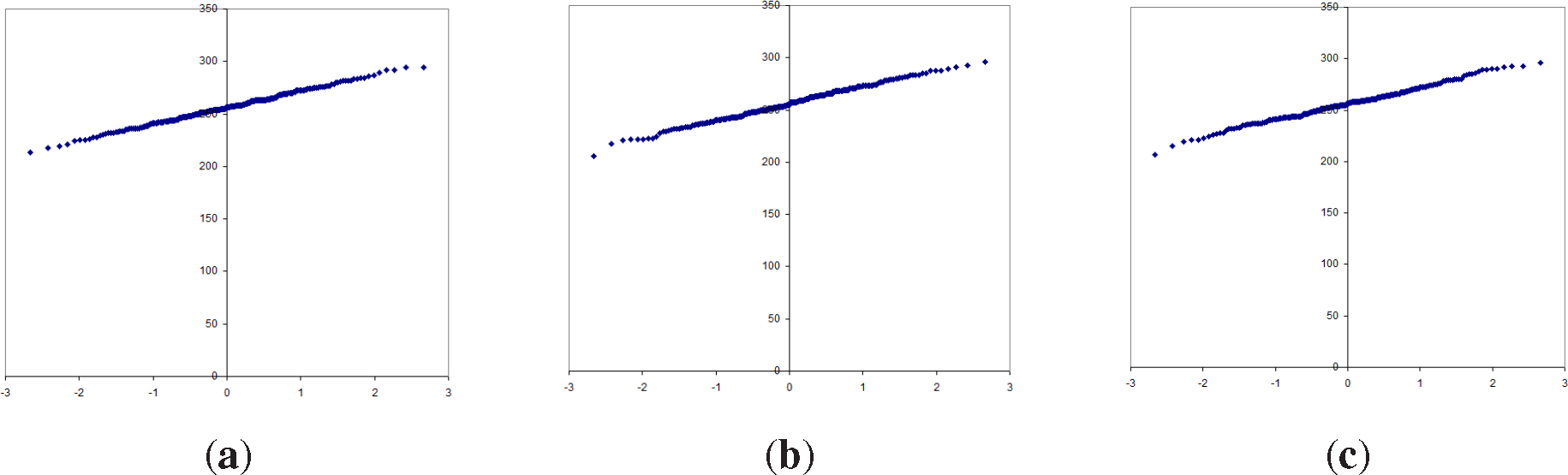
For mathematical quantity analysis of red, green and blue channels of the encrypted image 4.1.08 Jelly beans, we employed Kolmogorov–Smirnov Goodness-of-Fit Test to evaluate an uniformity. The normality was detected with Normal Quantile Plots (NormQuant.xls, Dr Scott Guth at Mt San Antonio College). The Fugure 4 shows the the Normal quantile plots. The obtained correlation coefficients of 0.999198758 (red histogram), 0.998107709 (green histogram), and 0.997868951 (blue histogram) are larger than critical values 0.989519603 (∝ = 0.01), 0.995880763 (∝ = 0.05), and 0.99710484 (∝ = 0.1). Therefore, the data follow the normal distribution. Similar results of uniformity are obtained in [29].

In addition of histogram analysis, the results of the average pixel intensity are given in

Table 5. Average pixel intensity of 24-bit color plain images and encrypted images.

File Name	24-bit Color Plain Image			24-bit Color Encrypted Image
	Red	Green	Blue	Red	Green	Blue
4.1.01	75.827	52.559	46.305	127.330	127.232	127.469
4.1.02	42.075	30.086	27.540	127.419	127.259	127.130
4.1.03	137.603	139.958	144.018	127.583	127.169	127.948
4.1.04	129.218	99.267	125.199	127.429	127.336	127.197
4.1.05	146.564	133.000	142.023	127.942	127.725	127.803
4.1.06	132.202	124.902	143.263	127.112	127.829	127.138
4.1.07	179.204	180.650	142.348	127.561	127.372	127.490
4.1.08	174.897	170.866	128.346	126.495	127.420	127.414
4.2.01	176.270	70.494	108.898	127.415	127.515	127.244
4.2.02	234.195	208.644	163.552	127.503	127.451	127.515
4.2.03	137.391	128.859	113.117	127.752	128.344	127.385
4.2.04	180.224	99.051	105.410	127.530	127.407	127.690
4.2.05	177.577	177.852	190.214	127.396	127.504	127.438
4.2.06	131.007	124.304	114.893	127.663	127.598	127.551
4.2.07	149.821	115.568	66.534	127.327	127.369	127.488
House	155.436	168.226	142.209	127.397	127.452	127.609

and

Table 6. Average pixel intensity of 8-bit grayscale plain images and encrypted images.

File Name	8-bit Grayscale Plain Image	8-bit Grayscale Encrypted Image
5.1.09	127.760	127.118
5.1.10	140.507	127.283
5.1.11	193.554	127.627
5.1.12	185.980	127.785
5.1.13	225.915	127.904
5.1.14	104.470	127.870
5.2.08	123.177	127.489
5.2.09	180.572	127.555
5.2.10	113.802	127.500
5.3.01	89.008	127.499
5.3.02	82.995	127.458
7.1.01	107.114	127.273
7.1.02	175.335	127.494
7.1.03	132.385	127.670
7.1.04	116.118	127.422
7.1.05	106.393	127.431
7.1.06	90.483	127.377
7.1.07	108.239	127.350
7.1.08	127.188	127.594
7.1.09	125.604	127.403
7.1.10	119.273	127.327
7.2.01	32.514	122.464
Boat	129.708	127.434
Elaine	136.357	127.422
Gray21	127.038	127.758
Numbers	103.519	127.350
Ruler	226.940	127.661
Testpat	124.616	127.589

. They validate the uniformity in distribution of red, green and blue channels of the encrypted images.

4.2.4. Information Entropy Analysis

The information entropy H(X) is a statistical measure of uncertainty in communication theory [30]. It is defined as follows:

$$H(X)=-{\displaystyle \sum _{i=0}^{255}p(x_i){\log }_{2}p(x_i),}$$

(5)

where X is a discrete random variable, p(x_i) is the probability density function of the occurrence of the symbol x_i. Let us consider that there are 256 values of the information source in red, green, blue, and grey colors of the image with the same probability. We can get the perfect entropy H(X) = 8, corresponding to a truly random sample.

The information entropy of red, green, blue and grey colors of the plain and their corresponding encrypted images are computed and displayed in

Table 7. Entropy results of 24-bit plain images and encrypted images.

File Name	24-bit Plain Image			24-bit Encrypted Image
	Red	Green	Blue	Red	Green	Blue
4.1.01	6.42005	6.44568	6.38071	7.99732	7.99712	7.99730
4.1.02	6.24989	5.96415	5.93092	7.99760	7.99713	7.99750
4.1.03	5.65663	5.37385	5.71166	7.99719	7.99711	7.99726
4.1.04	7.25487	7.27038	6.78250	7.99683	7.99700	7.99719
4.1.05	6.43105	6.53893	6.23204	7.99734	7.99682	7.99709
4.1.06	7.21044	7.41361	6.92074	7.99712	7.99739	7.99714
4.1.07	5.26262	5.69473	6.54641	7.99714	7.99621	7.99736
4.1.08	5.79199	6.21951	6.79864	7.99737	7.99714	7.99730
4.2.01	6.94806	6.88446	6.12645	7.99926	7.99936	7.99926
4.2.02	4.33719	6.66433	6.42881	7.96825	7.99941	7.99940
4.2.03	7.70667	7.47443	7.75222	7.99930	7.99934	7.99929
4.2.04	7.25310	7.59404	6.96843	7.99936	7.99935	7.99936
4.2.05	6.71777	6.79898	6.21377	7.99930	7.99937	7.99931
4.2.06	7.31239	7.64285	7.21364	7.99929	7.99930	7.99925
4.2.07	7.33883	7.49625	7.05831	7.99923	7.99922	7.99937
House	7.41527	7.22948	7.43538	7.99932	7.99932	7.99937

and

Table 8. Entropy results of 8-bit plain images and encrypted images.

File Name	8-bit Grayscale Plain Image	8-bit Grayscale Encrypted Image
5.1.09	6.70931	7.99718
5.1.10	7.31181	7.99717
5.1.11	6.45228	7.96999
5.1.12	6.70567	7.99757
5.1.13	1.54831	7.99735
5.1.14	7.34243	7.99674
5.2.08	7.20100	7.99934
5.2.09	6.99399	7.99930
5.2.10	5.70556	7.99926
5.3.01	7.52374	7.99983
5.3.02	6.83033	7.99981
7.1.01	6.02741	7.99929
7.1.02	4.00450	7.99931
7.1.03	5.49574	7.99925
7.1.04	6.10742	7.99923
7.1.05	6.56320	7.99929
7.1.06	6.69528	7.99933
7.1.07	5.99160	7.99931
7.1.08	5.05345	7.99923
7.1.09	6.18981	7.99219
7.1.10	5.90879	7.99937
7.2.01	5.64145	7.99984
Boat	7.19137	7.99928
Elaine	7.50598	7.99922
Gray21	4.39230	7.99932
Numbers	7.72925	7.99934
Ruler	0.50003	7.99927
Testpat	4.40773	7.99982

.

From the obtained results it is clear that the entropies of red, green, blue, and grey colors of the encrypted images are very close to the ideal value, which is an indication that the new chaos-based image encryption scheme is secure and credible upon information entropy attempt. In addition,

Table 9. Information entropy comparisons.

Encryption Algorithm	4.2.04 Lena			4.2.07 Peppers
	Red	Green	Blue	Red	Green	Blue
Proposed scheme	7.99936	7.99935	7.99936	7.99923	7.99922	7.99937
Reference [7]	7.98710	7.98810	7.98780	7.98770	7.98810	7.98770
Reference [31]	7.99930	8.00080	8.00070	–	–	–
Reference [32]	7.98970	7.98770	7.98960	7.98940	7.98840	7.98660
Reference [34]	7.99724	7.99683	7.99715	–	–	–
Reference [33]	7.99927	7.99924	7.99911	–	–	–

summarizes the information entropy values for Lena and Peppers encrypted images compared with values in [7,31–33]. As we can see that although they are all close to the ideal entropy value, the results of the novel algorithm are larger than those of corresponding methods.

4.2.5. Correlation Coefficient Analysis

Because of the existing correlation either in horizontal, vertical, or diagonal direction of the plain image pixels, the correlation coefficient r between two adjacent pixels (a_i, b_i) is computed [35].

$$r=\frac{\mathrm{cov}(a,b)}{\sqrt{D(a)}\sqrt{D(b)}},$$

(6)

where

$$D(a)=\frac{1}{M}{\displaystyle \sum _{i=1}^M{(a_i-\overline{a})}^2,}$$

(7)

$$D(b)=\frac{1}{M}{\displaystyle \sum _{i=1}^M{(b_i-\overline{b})}^2,}$$

(8)

$$\mathit{cov}(a,b)={\displaystyle \sum _{i=1}^M(a_i-\overline{a})(b_i-\overline{b}),}$$

(9)

M is the total number of couples (a_i, b_i), obtained from the image, and ā, $\overline{b}$ are the mean values of a_i and b_i, respectively. Correlation coefficient r can range in the interval of [−1.00, +1.00].

Table 10. Horizontal, vertical and diagonal correlation coefficients of adjacent pixels in the plain and encrypted images.

File Name	Plain Image Correlation			Encrypted Image Correlation
	Horizontal	Vertical	Diagonal	Horizontal	Vertical	Diagonal
4.1.01	0.971188	0.965984	0.949514	−0.000534	0.000234	−0.001845
4.1.02	0.930295	0.956492	0.900074	−0.000300	−0.003734	0.008957
4.1.03	0.974448	0.921184	0.896931	−0.007803	−0.010133	0.003399
4.1.04	0.973557	0.980473	0.961080	0.003453	−0.009509	−0.009399
4.1.05	0.978595	0.957145	0.945483	0.004011	−0.002541	0.002727
4.1.06	0.965978	0.937247	0.927815	0.001987	−0.002162	0.003613
4.1.07	0.982519	0.984660	0.970220	−0.003301	0.001817	−0.004506
4.1.08	0.974626	0.977833	0.952514	0.005680	−0.008603	−0.008341
4.2.01	0.980782	0.990701	0.974648	0.001730	−0.004172	0.001539
4.2.02	0.950537	0.912459	0.901982	−0.001518	−0.000623	0.003056
4.2.03	0.878222	0.784600	0.755893	0.003984	−0.004631	0.003949
.2.04	0.968723	0.983264	0.956063	−0.003761	0.001775	0.000686
4.2.05	0.966548	0.949166	0.932570	−0.001662	0.000894	0.003358
4.2.06	0.974732	0.972170	0.958270	−0.004090	−0.005167	0.000130
4.2.07	0.970430	0.977396	0.958278	−0.000116	−0.000307	−0.002276
House	0.958335	0.957411	0.928622	−0.002882	−0.004121	0.004594
5.1.09	0.899288	0.938482	0.901437	0.012628	−0.011439	−0.007696
5.1.10	0.901616	0.848045	0.818578	−0.002971	−0.000897	0.003682
5.1.11	0.955978	0.911356	0.891780	0.001757	−0.010444	0.001124
5.1.12	0.958841	0.973631	0.941568	0.009575	−0.002502	−0.000582
5.1.13	0.891950	0.849254	0.773639	0.000347	0.004691	−0.009999
5.1.14	0.946683	0.917624	0.852637	0.008773	−0.011971	0.000220
5.2.08	0.943933	0.868680	0.854776	−0.002389	−0.003528	−0.003059
5.2.09	0.900711	0.853424	0.803347	0.000783	−0.003316	−0.000207
5.2.10	0.941082	0.926039	0.898433	−0.006168	−0.007614	0.000369
5.3.01	0.977635	0.980525	0.967295	0.000606	0.000090	0.002417
5.3.02	0.909186	0.903231	0.858377	0.000502	0.001669	−0.000435
7.1.01	0.962015	0.920872	0.907585	−0.002843	0.000667	0.004116
7.1.02	0.946484	0.941026	0.895893	−0.003666	−0.001386	−0.001295
7.1.03	0.945493	0.929797	0.901696	−0.002931	−0.004124	0.003147
7.1.04	0.978887	0.966321	0.958102	−0.004028	−0.001065	−0.000901
7.1.05	0.941926	0.911431	0.893487	0.001735	−0.003046	−0.002081
7.1.06	0.940461	0.905249	0.886455	−0.001395	−0.003363	−0.001516
7.1.07	0.887121	0.879316	0.840438	−0.000608	0.000682	−0.000090
7.1.08	0.957101	0.929417	0.921126	−0.006136	−0.005571	0.003652
7.1.09	0.965857	0.929621	0.916903	−0.000695	−0.004547	−0.002457
7.1.10	0.964329	0.946928	0.931265	−0.000346	−0.001810	0.000957
7.2.01	0.964733	0.946692	0.944943	0.000677	0.000223	−0.001154
Boat	0.938283	0.971483	0.922259	0.001274	−0.003782	−0.000244
Elaine	0.975731	0.972933	0.969378	−0.001623	−0.002870	−0.001629
Gray21	0.996526	0.999838	0.996371	−0.000561	−0.002572	−0.000039
Numbers	0.768787	0.736467	0.634922	−0.005458	−0.002220	−0.003611
Ruler	0.544408	0.549529	0.003915	−0.001015	−0.004925	0.002669
Testpat	0.818682	0.841158	0.762415	0.001008	−0.001107	−0.001103

shows the results of horizontal, vertical, and diagonal adjacent pixels correlation coefficients computations of the plain images and the corresponding encrypted images. It is clear that the novel chaos based image encryption scheme does not keep any linear dependencies between observed pixels in all three directions: the inspected horizontal, vertical and diagonal correlation coefficients of the encrypted images are close to 0. Overall, the correlation coefficients of the proposed algorithm are analogous with results of four other image encryption schemes [10,25,27–29],

Table 11. Horizontal, vertical and diagonal correlation coefficients comparisons.

Encryption Algorithm	Image Correlation of Encrypted Image of 4.2.04 Lena
	Horizontal	Vertical	Diagonal
Proposed scheme	−0.003761	0.001775	0.000686
Reference [25]	0.019732	0.002467	0.004438
Reference [10]	−0.0574	−0.0035	0.0578
Reference [29]	0.0004	0.0021	−0.0038
Reference [27]	0.001354	−0.000254	−0.000327
Reference [28]	0.002016	−0.000916	0.001651

.

In addition, correlation coefficients between the corresponding pixel of the plain and their encrypted images are given in

Table 13. Correlation coefficients between the corresponding pixels of the plain and encrypted images—Columns 1, 2, 3, and 4. Correlation coefficients between the corresponding pixels of the encrypted images with keys K1 and K2—Columns 5, 6, 7, and 8.

File Name	Correlation Coefficient	File Name	Correlation Coefficient	File Name	Correlation Coefficient (K1,K2)	File Name	Correlation Coefficient (K1,K2)
4.1.01	0.00450439	5.2.08	−0.00177677	4.1.01	−0.0007753	5.2.08	−0.0008165
4.1.02	0.00039956	5.2.09	0.00163655	4.1.02	0.0037336	5.2.09	0.0000242
4.1.03	0.00386160	5.2.10	0.00285459	4.1.03	0.0003091	5.2.10	−0.0007335
4.1.04	0.00866526	5.3.01	−0.00032223	4.1.04	−0.0001636	5.3.01	−0.0002775
4.1.05	0.00353008	5.3.02	0.00055174	4.1.05	0.0049155	5.3.02	0.0013214
4.1.06	0.00202353	7.1.01	−0.00111200	4.1.06	−0.0047615	7.1.01	0.0026200
4.1.07	−0.00337130	7.1.02	−0.00232477	4.1.07	−0.0039018	7.1.02	0.0035445
4.1.08	−0.00339438	7.1.03	−0.00281014	4.1.08	0.0022217	7.1.03	0.0004484
4.2.01	−0.00078462	7.1.04	0.00220779	4.2.01	0.0002696	7.1.04	0.0011823
4.2.02	−0.00148823	7.1.05	0.00051300	4.2.02	−0.0021341	7.1.05	−0.0015177
4.2.03	−0.00016366	7.1.06	0.00000058	4.2.03	−0.0008931	7.1.06	0.0041168
4.2.04	−0.00032519	7.1.07	−0.00137758	4.2.04	0.0032183	7.1.07	−0.0008043
4.2.05	0.00044032	7.1.08	−0.00051899	4.2.05	0.0046435	7.1.08	0.0047454
4.2.06	−0.00324635	7.1.09	−0.00030899	4.2.06	−0.0024745	7.1.09	−0.0010962
4.2.07	−0.00058506	7.1.10	0.0025460	4.2.07	−0.0000077	7.1.10	−0.0027879
House	−0.00252335	7.2.01	0.00170215	House	0.0009227	7.2.01	−0.0000272
5.1.09	0.00243208	Boat	−0.00425251	5.1.09	−0.0020602	Boat	−0.0011746
5.1.10	−0.00025318	Elaine	0.00280115	5.1.10	0.0024437	Elaine	−0.0017324
5.1.11	−0.00365694	Gray21	0.00348155	5.1.11	0.0021018	Gray21	0.0023155
5.1.12	−0.00179198	Numbers	0.00124149	5.1.12	0.0000859	Numbers	0.0009983
5.1.13	0.00302971	Ruler	0.00037308	5.1.13	−0.0051945	Ruler	−0.0007557
5.1.14	0.00056840	Testpat	−0.00010024	5.1.14	0.0010020	Testpat	−0.0010965

(Columns 1, 2, 3, and 4). The computed correlation values are very close to 0.00.

4.2.6. Differential Attack

In general, a common characteristic of an image encryption scheme is to be sensitive to minor modifications in the plain images. Differential analysis allows that an adversary is able to create small changes in the plain image and revise the encrypted image. The alternation level can be computed by means of two formulae, namely, the number of pixels change rate (NPCR) and the unified average changing intensity (UACI) [35,36].

Let us assume encrypted images before and after one pixel modification in a plain image are C₁ and C₂. The NPCR and UACI are defined as follows:

$$NPCR=\frac{{\displaystyle {\sum }_{i=0}^{W-1}{\displaystyle {\sum }_{j=0}^{H-1}D(i,j)}}}{W\times H}\times 100\%,$$

(10)

$$UACI=\frac{1}{W\times H}\left({\displaystyle \sum _{i=0}^{W-1}{\displaystyle \sum _{j=0}^{H-1}\frac{|C_1(i,j)-C_2(i,j)|}{255}}}\right)\times 100\%,$$

(11)

where D is a two-dimensional set, having the same size as image C₁ or C₂, and W and H are respectively the width and height of the image. The set D(i, j) is defined by C₁(i, j) and C₂(i, j), if C₁(i, j) = C₂(i, j) then D(i, j) = 1; otherwise, D(i, j) = 0. The NPCR and UACI test results from the proposed chaos based algorithm are shown in

Table 12. NPCR and UACI results of encrypted 24-bit plain images and encrypted with one pixel difference 24-bit plain images.

File Name	NPCR Test			UACI Test
	Red	Green	Blue	Red	Green	Blue
4.1.01	99.5987	99.6307	99.5941	33.3430	33.4454	33.4751
4.1.02	99.5804	99.6124	99.5758	33.3778	33.4066	33.4268
4.1.03	99.5789	99.5926	99.6155	36.3228	33.5826	33.4725
4.1.04	99.6262	99.5880	99.5728	33.6492	33.4109	33.4568
4.1.05	99.5773	99.5758	99.6368	33.3521	33.4299	33.4417
4.1.06	99.5819	99.5453	99.5605	33.4896	33.3675	33.3237
4.1.07	99.6048	99.5865	99.6124	33.5262	33.6109	33.4652
4.1.08	99.5743	99.5621	99.6201	33.5528	33.5090	33.4787
4.2.01	99.6174	99.5922	99.5911	33.4989	33.5431	33.4665
4.2.02	99.6113	99.6094	99.6094	33.4586	33.4940	33.4936
4.2.03	99.6334	99.5998	99.6208	33.4858	33.5439	33.5361
4.2.04	99.6021	99.6075	99.6029	33.4693	33.5366	33.5408
4.2.05	99.6120	99.6155	99.6040	33.4792	33.4006	33.3745
4.2.06	99.6155	99.6147	99.5914	33.4927	33.5608	33.4377
4.2.07	99.6014	99.6311	99.5895	33.4260	33.4912	33.4121
House	99.6307	99.5995	99.6063	33.5282	33.5377	33.4830

and

Table 15. NPCR and UACI results of encrypted 8-bit plain images and encrypted with one pixel difference 8-bit plane images—Column 2 and Column 3; NPCR and UACI results of encrypted 8-bit plain images with keys K1 and K2—Column 4 and Column 5.

File Name	NPCR Test(1px)	UACI Test(1px)	NPCR Test(K1,K2)	UACI Test(K1,K2)
5.1.09	99.5804	33.4011	99.5804	33.4004
5.1.10	99.5560	33.4318	99.5560	33.4312
5.1.11	99.6124	33.4197	99.6124	33.4191
5.1.12	99.5697	33.4589	99.5697	33.4592
5.1.13	99.5972	33.3431	99.5972	33.3424
5.1.14	99.6216	33.4044	99.6216	33.4050
5.2.08	99.5998	33.5342	99.5998	33.5342
5.2.09	99.6311	33.3784	99.6311	33.3783
5.2.10	99.6059	33.4327	99.6059	33.4326
5.3.01	99.5980	33.4848	99.5980	33.4848
5.3.02	99.6048	33.4401	99.6048	33.4401
7.1.01	99.5953	33.4850	99.5953	33.4851
7.1.02	99.6040	33.4916	99.6040	33.4915
7.1.03	99.6204	33.5177	99.6240	33.5179
7.1.04	99.6117	33.4487	99.6117	33.4487
7.1.05	99.6002	33.4820	99.6002	33.4821
7.1.06	99.6029	33.4817	99.6029	33.4819
7.1.07	99.6170	33.4932	99.6170	33.4934
7.1.08	99.5945	33.4963	99.5945	33.4961
7.1.09	99.6063	33.4840	99.6063	33.4842
7.1.10	99.6063	33.4246	99.6063	33.4244
7.2.01	99.6170	33.4214	99.6170	33.4214
Boat	99.6204	33.5708	99.6204	33.5707
Elaine	99.5968	33.4186	99.5968	33.4186
Gray21	99.6086	33.3906	99.6086	33.3909
Numbers	99.6124	33.4232	99.6124	33.4231
Ruler	99.6208	33.4196	99.6208	33.4197
Testpat	99.6083	33.4537	99.6083	33.4537

(Columns 2 and 3).

The obtained NPCR and UACI values for all of the images are larger than the critical values proposed in [36] and similar to the values presented in [10]. The values point out that the novel image encryption algorithm is vastly sensitive regarding to small changes in the plain images and has a vigorous strength of contrary differential cryptanalysis.

4.2.7. Key Sensitivity Test

The strong key sensitivity is another characteristic of the correlation analysis. a good image encryption scheme should be sensitive regarding the secret key i.e. a negligible change of the secret key. We encrypted the 48 images with two similar secret keys: K1 and K2 (x₀ = 0.2343214592, y₀ = −0.742190593, T₁(x₁) = 0.7029381194009314, T₁(x₂) = −0.3001928364928377, T₁(x₃) = 0.1385946382912478, and T₁(x₄) = −0.2871955600387584). The results are shown in Table 13 (Columns 5, 6, 7, and 8). It is clear that the novel image encryption method is strong key sensitive: the correlation coefficients are relatively close to zero.

Moreover, another round of the NPCR and UACI tests are established. In this case, C₁ and C₂ are two encrypted images, obtained from one plain image by the novel encryption scheme using the keys K1 and K2. The results are displayed in

Table 14. NPCR and UACI results of encrypted 24-bit plain images with keys K1 and K2.

File Name	NPCR test			UACI test
	Red	Green	Blue	Red	Green	Blue
4.1.01	99.5987	99.6307	99.5941	33.3431	33.4459	33.4754
4.1.02	99.5804	99.6124	99.5758	33.3770	33.4070	33.4269
4.1.03	99.5789	99.5926	99.6155	36.3286	33.5835	33.4727
4.1.04	99.6262	99.5880	99.5728	33.6493	33.4110	33.4559
4.1.05	99.5773	99.5758	99.6368	33.3530	33.4299	33.4408
4.1.06	99.5819	99.5753	99.5605	33.4900	33.3662	33.3242
4.1.07	99.6048	99.5865	99.6124	33.5258	33.6110	33.4658
4.1.08	99.5743	99.5621	99.6201	33.5517	33.5094	33.4779
4.2.01	99.6174	99.5922	99.5911	33.4989	33.5430	33.4663
4.2.02	99.6113	99.6094	99.6094	33.4586	33.4941	33.4933
4.2.03	99.6334	99.5998	99.6208	33.4858	33.5438	33.5259
4.2.04	99.6021	99.6075	99.6029	33.4693	33.5368	33.5406
4.2.05	99.6120	99.6155	99.6040	33.4792	33.4007	33.3744
4.2.06	99.6155	99.6147	99.5941	33.4925	33.5609	33.4380
4.2.07	99.6014	99.6311	99.5895	33.4262	33.4909	33.4121
House	99.6307	99.5995	99.6063	33.5284	33.5374	33.4830

and 15 (Columns 4 and 5).

In addition, in Figure 5, the results of two tests are shown to decrypt the encrypted with key K1 4.1.07 and 7.1.03 images, Figure 5e and Figure 5f, with the secret key K2.

We observed that the two decrypted images Figure 5e and Figure 5f have no relation with the plain images 4.2.07 and 7.1.03, Figure 5a and Figure 5b, respectively.

4.2.8. Computational and Complexity Analysis

We have measured the average encryption time for 512 × 512 sized grayscale and color images by using the proposed image encryption algorithm. Computational analysis has been done on a 2.40 GHz Intel ® Core™ i7-3630QM Dell Inspiron laptop. The results are provided in

Table 16. Time complexity comparisons.

Encryption Algorithm	Average Time (ms)
	Grayscale	Color
Proposed scheme	95	290
Reference [37]	105	312
Reference [38]	130	389
Reference [25]	341	1019
Reference [27]	224	296
Reference [28]	35	105

. One can see from Table 16 that the novel image encryption algorithm runs slower only than algorithm in Reference [28]. The novel algorithm needs Θ(n²) of pixel shuffling iterations. For analysis of theoretical complexity in substitutions, the time-consuming parts in computations are Θ(n²) iterations of calculations of a sine and a cosine functions. Therefore, the proposed encryption scheme needs more theoretical time than the algorithms in [27,28].

Compared to other chaotic image encryption algorithms, we can see that the running speed of the proposed scheme is fast.

5. Conclusions

A novel image encryption scheme based on the theory of chaos is proposed in this communication. The suggested technique combines Chebyshev polynomial based permutation, and rotation equation based substitution. a strict security analysis on the novel scheme is given.

Detailed security analysis has been provided on the novel image encryption algorithm using visual testing, key space evaluation, histogram analysis, information entropy calculation, correlation coefficient analysis, differential analysis, key sensitivity test, and computational and complexity analysis.

Based on the obtained results, we can conclude that the proposed chaos based image encryption algorithm is reasonable for the secure image communication.

References

- Fridrich, J. Symmetric Ciphers Based on Two-Dimensional Chaotic Maps. Int. J. Bifurc. Chaos. 1998, 8, 1259–1284. [Google Scholar]
- Fu, C.; Wang, P.; Ma, X.; Xu, Z.; Zhu, W. A Fast Pseudo Stochastic Sequence Quantification Algorithm Based on Chebyshev Map and Its Application in Data Encryption, Proceedings of the 6th International Conference on Computational Science, Reading, UK, 28–31 May 2006.Computational Science–ICCS 2006; Alexandrov, V.; Albada, G.; Sloot, P.; Dongarra, J. (Eds.) Springer Verlag: Berlin, Germany, 2006; Lecture Notes in Computer Science 3991; pp. 826–829.
- Fu, C.; Chen, J.; Zou, H.; Meng, W.; Zhan, Y.; Yu, Y. A Chaos-Based Digital Image Encryption Scheme with an Improved Diffusion Strategy. Opt. Express. 2012, 20, 2363–2378. [Google Scholar]
- Hung, X. Image encryption algorithm using chaotic Chebyshev generator. Nonlinear Dyn. 2012, 67, 2411–2417. [Google Scholar]
- Yoon, E.; Jeon, I. An efficient and secure Diffie-Hellman key agreement protocol based on Chebyshev chaotic map. Commun. Nonlinear Sci. Numer. Simul. 2011, 16, 2383–2389. [Google Scholar]
- Wang, X.; Teng, L.; Qin, X. A NovelColour Image Encryption Algorithm Based on Chaos. Signal Process. 2012, 92, 1101–1108. [Google Scholar]
- Fu, C.; Lin, B.; Miao, Y.; Liu, X.; Chen, J. A NovelChaos-Based Bit-Level Permutation Scheme for Digital Image Encryption. Opt. Commun. 2011, 284, 5415–5423. [Google Scholar]
- Wang, X.-Y.; Yang, L.; Liu, R.; Kadir, A. A chaotic image encryption algorithm based on perceptron model. Nonlinear Dyn. 2010, 62, 615–621. [Google Scholar]
- Wang, X.-Y.; Yu, Q. A block encryption algorithm based on dynamic sequences of multiple chaotic systems. Commun. Nonlinear Sci. Numer. Simul. 2009, 14, 574–581. [Google Scholar]
- Liu, H.; Wang, X. Color image encryption using spatial bit-level permutation and high-dimension chaotic system. Opt. Commun. 2011, 284, 3895–3903. [Google Scholar]
- Skiadas, C.H. Mathematical models of Chaos. In Chaos Applications in Telecommunications; Stavroulakis, P., Ed.; CRC Press: Boca Raton, FL, USA, 2006; pp. 383–413. [Google Scholar]
- Skiadas, C.H.; Skiadas, C. Chaotic Modelling and Simulation: Analysis of Chaotic Models, Attractors and Forms; CRC Press: Boca Raton, FL, USA, 2008. [Google Scholar]
- Rukhin, A.; Soto, J.; Nechvatal, J.; Smid, M.; Barker, E.; Leigh, S.; Levenson, M.; Vangel, M.; Banks, D.; Heckert, A.; et al. A Statistical Test Suite for Random and Pseudorandom Number Generators for Cryptographic Application; NIST Special Publication 800-22; NIST: Gaithersburg, MD, USA, 15 May 2001. [Google Scholar]
- Marsaglia, G. The Marsaglia Random Number CDROM including the Diehard Battery of Tests of Randomness; Florida State University: Tallahassee, FL, USA, 1995. Available online: http://www.stat.fsu.edu/pub/diehard/ accessed on 8 April 2015.
- Walker, J. ENT: A Pseudorandom Number Sequence Test Program. Available online: http://www.fourmilab.ch/random/ accessed on 8 April 2015.
- Hell, M.; Johansson, T.; Meier, W. Grain: A stream cipher for constrained environments. Int. J. Wirel. Mobile Comput. 2007, 2, 86–93. [Google Scholar]
- Kocarev, L.; Makraduli, J.; Amato, P. Public-Key Encryption Based on Chebyshev Polynomials. Circuits Syst. Signal Process. 2005, 24, 497–517. [Google Scholar]
- Kordov, K.M. Modified Chebyshev map based pseudo-random bit generator. AIP Conf. Proc. 2014, 1629, 432–436. [Google Scholar]
- Stoyanov, B.P. Pseudo-random bit generator based on Chebyshev map. AIP Conf. Proc. 2013, 1561, 369–372. [Google Scholar]
- Stoyanov, B.; Kordov, K. Novel Image Encryption Scheme Based on Chebyshev Polynomial and Duffing Map. Sci. World J 2014. [Google Scholar] [CrossRef]
- IEEE Computer Society, IEEE Standard for Binary Floating-Point Arithmetic. ANSI/IEEE Std. 754; IEEE: New York, NY, USA, 1985.
- Chen, J.; Zhu, Z.; Fu, C.; Yu, H. An Improved Permutation-Diffusion Type Image Cipher with a Chaotic Orbit Perturbing. Opt. Express. 2013, 21, 27873–27890. [Google Scholar]
- Diaconu, A.; Loukhaoukha, K. An Improved Secure Image Encryption Algorithm Based on Rubik’s Cube Principle and Digital Chaotic Cipher. Math. Probl. Eng. 2013. [Google Scholar] [CrossRef]
- Gao, H.; Zhang, Y.; Liang, S.; Li, D. A new chaotic algorithm for image encryption. Chaos Solitons Fractals. 2006, 29, 393–399. [Google Scholar]
- Lian, S.G.; Sun, J.; Wang, Z. A block cipher based on a suitable use of the chaotic standard map. Chaos Solitons Fract. 2005, 26, 117–129. [Google Scholar]
- Al-Maadeed, S.; Al-Ali, A.; Abdalla, T. A New Chaos-Based Image-Encryption and Compression Algorithm. J. Electr. Comp. Eng. 2012, 2012. [Google Scholar] [CrossRef]
- Zhang, Y.-Q.; Wang, X.-Y. A symmetric image encryption algorithm based on mixed linear-nonlinear coupled map lattice. Inf. Sci. 2014, 273, 329–351. [Google Scholar]
- Zhu, Z.-L.; Zhang, W.; Wong, K.W.; Yu, H. A chaos-based symmetric image encryption scheme using a bit-level permutation. Inf. Sci. 2011, 181, 1171–1186. [Google Scholar]
- Liu, H.; Wang, X.; Kadir, A. Image encryption using DNA complementary rule and chaotic maps. Appl. Soft. Comput. 2012, 12, 1457–1466. [Google Scholar]
- Shannon, C.E. A Mathematical Theory of Communication. Bell Syst. Tech. J 1948, 27. [Google Scholar]
- He, J.; Li, Z.-B; Qian, H.-F. Cryptography based on Spatiotemporal Chaos System and Multiple Maps. J. Softw. 2010, 5, 421–428. [Google Scholar]
- Liu, L.; Zhang, Q.; Wei, X. A RGB image encryption algorithm based on DNA encoding and chaos map. Comput. Electr. Eng. 2012, 38, 1240–1248. [Google Scholar]
- Seyedzadeh, S.M.; Mirzakuchaki, S. A fast color image encryption algorithm based on coupled two-dimensional piecewise chaotic map. Signal Process. 2012, 92, 1202–1215. [Google Scholar]
- Mazloom, S.; Eftekhari-Moghadam, A.M. Color image encryption based on coupled nonlinear chaotic map. Chaos Solitons Fractals. 2009, 42, 1745–1754. [Google Scholar]
- Chen, G.; Mao, Y.; Chui, C.K. A Symmetric Image Encryption Scheme Based on 3D Chaotic Cat Maps. Chaos Solitons Fractals. 2004, 21, 749–761. [Google Scholar]
- Wu, Y.; Noonan, J.P.; Agaian, S. NPCR and UACI Randomness Tests for Image Encryption. Cyber J. Multidiscip. J. Sci. Technol. J. Sel. Areas Telecommun. 2011, 2, 31–38. [Google Scholar]
- Ghebleh, M.; Kanso, A.; Noura, H. An image encryption scheme based on irregularly decimated chaotic maps. Signal Process. Image Commun. 2014, 29, 618–627. [Google Scholar]
- Kanso, A.; Ghebleh, M. A novel image encryption algorithm based on a 3D chaotic map. Commun. Nonlinear Sci. Numer. Simul. 2012, 17, 2943–2959. [Google Scholar]
Figure 1.
Rotation equations with
x0 = 0.5,
y0 = 1.0,
θ = 2,
a = 2.8,
rt = 10.3 and 20,000 iterations of
Equation (1).
Figure 2.
Comparison of the plain image and the encrypted image: (a) original picture 4.2.06 Sailboat on lake; (b) encrypted image of 4.2.06 Sailboat on lake.
Figure 3.
Histogram analysis of plain image and encrypted image: (a), (c), and (e) show the histograms of red, green, and blue channels of the plain picture 4.1.08 Jelly beans; (b), (d), and (f) show the histograms of red, green, and blue channels of encrypted picture 4.1.08 Jelly beans.
Figure 4.
Kolmogorov–Smirnov test of the histograms of the encrypted image 4.1.08 Jelly beans: (a), (b), and (c) show the Normal quantile plots of the red, green, and blue histograms.
Figure 5.
Key sensitive analysis of the plain images 4.2.07 and 7.1.03, (a) and (b), encrypted with the key K1, (c) and (d), and decrypted with the key K2, (e) and (f).