2. One-Dimensional Dynamical Model of Electron Transfer
Long-range electron tunneling through biomolecules (e.g., azurin and DNA) has been studied in substantial detail both experimentally and theoretically over the past twenty years [
2,
4,
15,
16,
17,
18,
19,
20]. In previous work, [
11,
12,
13,
14,
21,
22,
23,
24,
25,
26,
27] we studied the influence of nonlinear lattice excitations on electron transfer (ET). It was shown that electron trapping by solitons and a new form of electron transport mediated by solitons is possible in an anharmonic 1d lattice. Here, we focus attention on the process that occurs between two units in the chain, the donor D and the acceptor A, with in-between a bridge consisting of n elements denoted by b: D-b-b-b-b-b.........-b-b-b-A. We shall show that solitons may help to transfer electrons along the bridge. We will not consider in detail the processes D-b and b-A, referring to the literature [
17,
18].
If solitons are excited by an external source, stable bound states of electrons and solitons may be formed, which may move with supersonic or slightly subsonic velocity. In a heated system, solitons are excited thermally. These solitons and the corresponding solectrons have a finite life time and change their direction stochastically. The electrons may surf on thermal solitons from donor to acceptor. Under these conditions, we may consider the ET as a process similar to a diffusion-controlled reaction.
Building upon earlier work [
11,
12,
13,
14,
21,
22,
23,
24,
25,
26,
27], our interest is here in developing a dynamical theory which allows the description of ET over long distances, including the influence of thermal excitations. Adopting a 1d nonlinear lattice model to portray the backbone of the biomolecular chain (polypeptide, polynucleotide or other), we investigate the consequences of nonlinear, running, lattice excitations on electron transport. The theoretical model studied here is based the quantum mechanical “tight binding” approximation (TBA) [
28] for the electrons which are moving on a lattice with Morse interactions. Note that the use of Morse potentials is just for numerical convenience and is not a must for the results. We study in detail the role of thermal factors on electron transfer and the transition times, and give a thorough discussion of the role of nonlinearity. One of the tasks is to develop a simple model based on the Smoluchowski–Chandrasekhar picture of diffusion-controlled reactions as stochastic processes with emitters and absorbers. We estimate the time-distance relations for the new non-standard mechanisms of ET and the dependence on temperature at moderate temperatures. The lattice interactions allow for phonon-and soliton-longitudinal vibrations with compressions governed by the repulsive part of the potential [
11,
12,
13,
14,
29,
30,
31,
32]. Thus, we consider a 1d anharmonic lattice with dynamics described by the following Hamiltonian:
. The lattice part includes nearest-neighbor Morse interactions:
Here, M denotes the mass of a lattice unit (all units have equal mass), the coordinates and momenta ; describe their respective displacements from equilibrium positions () and momenta, B characterizes the stiffness of the spring-like constant in the Morse potential, D is the depth of the potential well, and σ defines equilibrium lattice spacing. These compressions were shown to be responsible for electron trapping by the lattice excitations thus leading to the formation of dynamic bound states (solectrons) of the electron with the soliton (the same phenomenon is valid also for the solitonic peaks of a periodic cnoidal wave moving through the lattice). Furthermore, we consider the whole system in a “thermal bath” characterized by a Gaussian white noise, , of zero mean and delta-correlated.
We add electrons to the system of Morse particles assuming that the electrons are in reality in 3d space though the lattice is 1d. Thus, for the electron-lattice dynamics, we have
where
n denotes the site where one electron is “placed” on the lattice, the complex numbers
give the
n-th component of the wave function and
gives the probability of finding the electron residing at the site
n. The bound state energy at site
n may depend on the relative distances between neighbors. We will use the ansatz
This is a translation-invariant modification of the linear shift used by Holstein and Kalosakas
et al. [
33,
34]. In view of its minor role, in what follows, we shall neglect the second term in Equation (
3). With this approximation, we want to keep the effect of energy shifts rather small, concentrating more on the influence on the transfer elements. The quantity
defines the transfer matrix element or overlapping integral responsible for the transport of the electron along the chain (considering only nearest neighbors). This matrix is the key ingredient, allowing for the coupling of the electron to the lattice displacements, and hence the lattice vibrations, phonons or solitons. Following Slater [
35,
36,
37], we take
where the parameter
accounts for the strength of the coupling added to parameter
. If we measure all energies in units 2D, it is convenient to measure also the energy levels in these
which gives
For the sake of universality, it is best to rescale quantities and consider a dimensionless problem. We take as unit of time,
, where
denotes the frequency of harmonic oscillations (linear, first-order approximation to the Morse exponential). For displacements, we take
as the unit, for momenta we take
, hence for the interaction force we have
, and
is measured in
units. Then, expecting no confusion in the reader, denoting the new dimensionless quantities with the same symbols as the old ones, the dynamics of the Hamiltonian system Equations (
1) and (
2), is given by the following equations for the components of the electronic wave function electron
, and the lattice vibrations,
where
Not counting the energy levels, there are four parameters, the last one relates the time scales of the electron and lattice dynamics. Needless to say, in general, the two time scales are not the same (which in frequency terms refer to ultraviolet/electronic
versus infrared/acoustic), for most cases with electrons and phonons. Instead of the ansatz Equation (
3), other equivalent expressions may be used [
12,
38,
39,
40]. For purposes of illustration, we take the following parameter values:
These numerical values are relevant, e.g., for electron transport along hydrogen bonded polypeptide chains such as
α-helices [
9,
25,
26,
27,
38,
39,
40,
41,
42]. Let us note what Muto
et al. [
43] give for DNA other values, which, in our model, correspond to:
3. Electrons Surfing on Solitons—A Guided Tour of Electrons from Donor to Acceptor
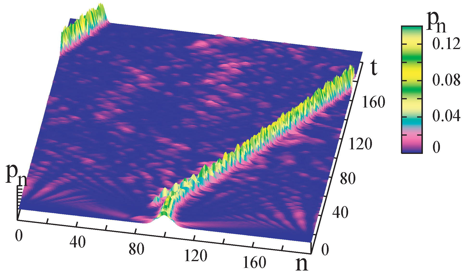
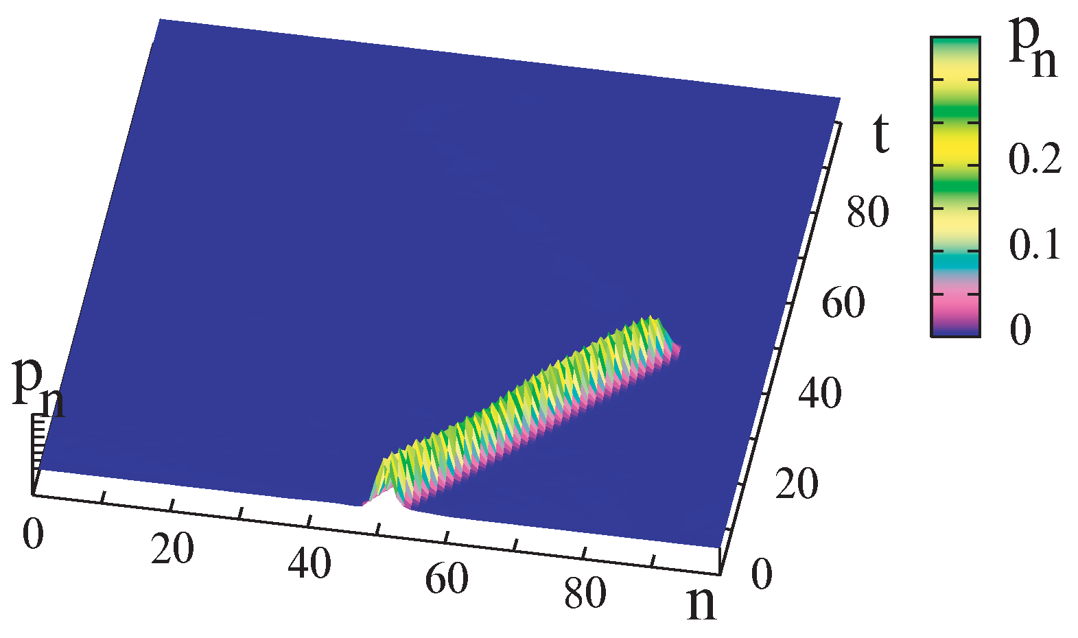
We shall estimate how the path of an electron may be influenced by a lattice soliton which was generated by an external perturbation of the lattice. The added, excess electron is placed at
at a donor located at site
at time
(
Figure 1). Due to the electron-lattice interaction (
), we observe soliton-assisted ET. The electron is dynamically bound to the soliton thus creating the travelling supersonic or slightly subsonic solectron excitation. Indeed when the electron-lattice interaction is operating, we see that the electron moves with the soliton with a slightly subsonic velocity
and is running to the right border of the square (
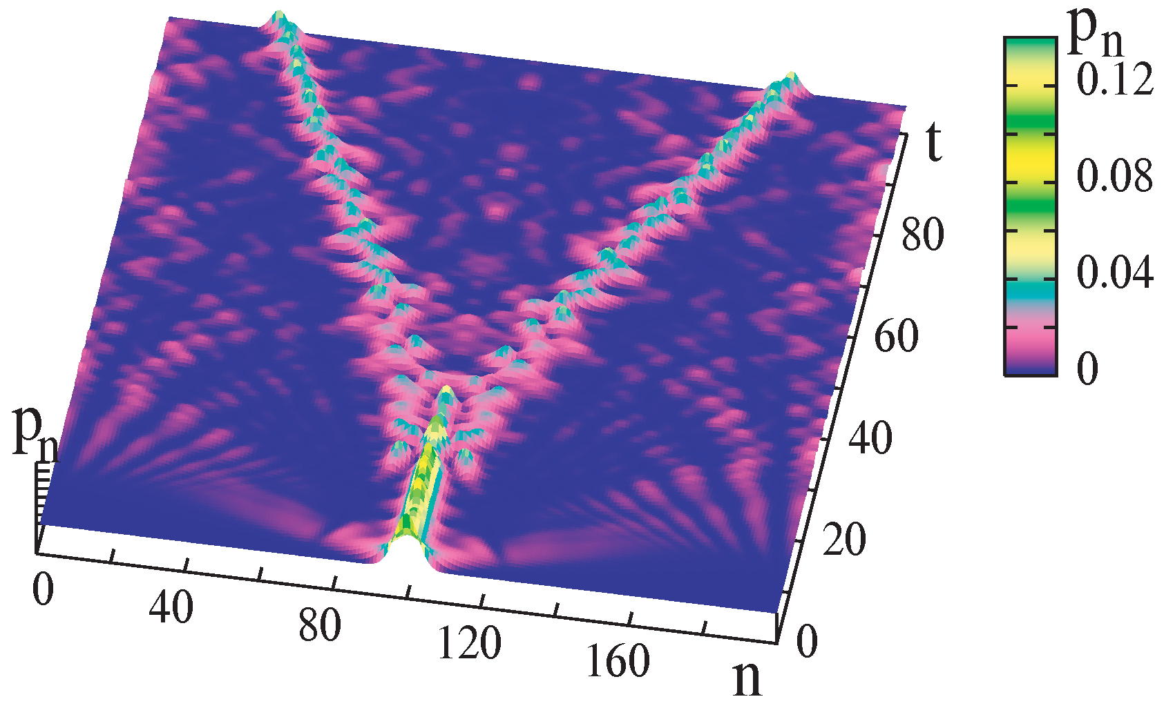
) plot. Let us assume that an acceptor is located there. This means that the electron is guided by the soliton from donor to acceptor. Note that, in transport processes, several solitons may be involved including those moving in opposite direction. Therefore, the above given soliton velocity is an upper bound for the soliton-assisted ET. In order to study the superposition of several solitons acting on one electron, we studied, in another experiment, the evolution of an electron in the presence of two solitons.
Figure 2 illustrates the splitting of the electron probability density. The existence of bound states between electrons and lattice deformations in 1d-lattices has been first studied in the continuous picture by Davydov and his school [
41,
44].
In principle, the above solectron effect may be used as a way to manipulate or otherwise to control the transport of electrons between donor and acceptor. Clearly, in our case, we may have a polaron-like effect due to the electron-phonon (or soliton) interaction coupled to a genuinely added lattice solitonic effect due to the anharmonicity of the lattice vibrations. This permits soliton rather than phonon-assisted long range hopping.
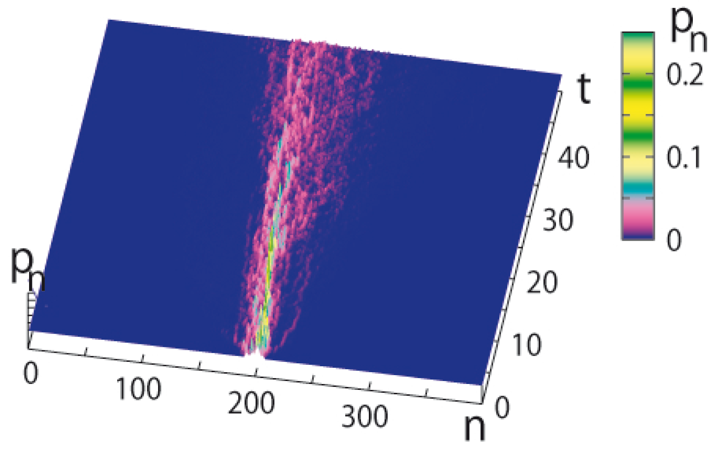
4. Dynamics of Electrons Interacting with Thermal Solitons
Let us study now a lattice heated to some temperature
T. Then, thermal solitons are excited due to the influence of thermal energy-rich collisions. However, we do not have just one or two solitons, but many of them are generated by the heat bath [
38,
39,
40]. To be expected is that this completely changes the picture. In previous work, we have shown that we do not find any more long-living soliton excitations in the chain [
24]. Instead, we see up to the range of physiological temperatures many small local soliton portions in the system which have a finite lifetime up to a few picoseconds. The electron probability density may split between all of them.
The general picture is now that the electron probability density is concentrated in the local “hot spots” created by the local soliton thermal excitations. In order to study the influence of this effect on donor-acceptor ET in more detail, we performed a series of computer simulations. In this series of experiments, we release an electron into an already heated lattice by means of the friction and noise sources. These sources are switched off at an instant that we now denote
. In
Figure 3, we represent the electron probability density developing in a lattice heated up to
. We see that the electron density is for
confined more or less in a cone. A similar picture is obtained for
, with a mere narrowing of the evolutionary cone. Clearly, the electron probability density splits into many small spots which are localized at thermally excited solitons. These “hot spots” comprise up to 10 lattice (take up to 50 Å) sites and have a short life time which is in the range of a few picoseconds. The little maximum of the electron density “dies” with the soliton or without destruction of the latter and moves eventually to the next nearby soliton. The whole process is time dependent as the “hot spots” are created and annihilated in the thermal process. Note that the spots denote only probabilities; in reality, the electron is localized at one of the spots.
Modeling the netto-transfer of the electrons theoretically is rather difficult due to the complexity of the life of an electron after injection. At first glance at the temperatures which we study here, it looks like a diffusion-like process. Let us discuss whether the ET is a proper diffusion process. As is well known, according to a linear Schrödinger equation, the electron probability density spreads in some respect similar to a diffusion process, meaning that the mean square displacement growths linearly in time. On the other hand, as shown by Brizhik and Davydov [
44], the nonlinear Schrödinger equation corresponds to processes which are much more complicated, e.g., the spreading of the density may be fractal-like and may depend on the initial conditions. This way, we cannot expect that the ET is at
or near to zero temperature a diffusion-like in all respects. Being aware of this complication, we take here a diffusion approach for temperatures
, or more precisely
(in units 2D), since we expect that the thermal motion smoothes the expansion processes. Possible complications at low
T including tunneling have been discussed elsewhere [
13,
14]. The quantum-mechanical processes at low temperatures, in particular the tunneling at
, is certainly not diffusion-controlled. In order to decide the question of whether the ET-processes at finite temperatures are diffusion-like, we have to study in more detail the mean square displacement of the spreading of a free electron on the heated lattice.
5. Mean Square Displacement of Electrons
For simplicity, we place the injected electron initially at
at
(for simplicity). The mean square displacement is given by
where the quantities
have to be calculated according to the discrete Schrödinger Equation (
6). This procedure gives, however, only the quantum-mechanical mean. Still, we need here a second average with respect to the stochastic trajectories of the lattice according to Equation (
10). This way, we define a diffusion-function of time
The outer bracket means that we have to take the average over many realizations (time evolutions) of the lattice dynamics. The result has to be drawn as a function of time. We expect that this function is linear in time at least in certain temperature range, that is,
. This is confirmed by computer simulations (
Figure 4). For the case of a linear lattice model, the linear dependence of the mean square displacement with time was obtained by Lakhno and collaborators [
45,
46].
The results of a stochastic simulation based on the master equation is shown by the thin line in
Figure 5 [
38,
39,
40] together with
derived using the Schrödinger equation (fat points). We see that both approaches disagree at low temperatures. As far as we see, the (theoretical) diffusion coefficient of the hopping process at
(no lattice dynamics) should be
τ (or may be proportional to
τ). Therefore, we believe that the calculation of
d Equation (
11) at low
with the Schrödinger equation is incorrect due to the problems of fractality and other difficulties with the Schrödinger equation [
8]. In order to avoid all these difficulties, as already said, we concentrate in this work only on
, where the two approaches go together. In the TBA, we model a heat bath corresponding to a temperature
T by introducing a Langevin source for the temperature and wait for complete thermalization. Then, we switch-off the heat bath,
i.e., the stochastic source and friction, and start with the initial conditions for velocities and positions the simulations of the coupled TBA-Hamiltonian system. This procedure guarantees for a short simulation time thermal conditions. In the case of using a master equation the method corresponds to a standard Monte-Carlo thermalization. For the diffusional regime, the diffusion theory is telling us that an electron initially concentrated at the position
has an evolving probability density described by
If we identify
with the donor, this formula shows how the electron probability density evolves at some distance, in particular, also at the place where the absorber is located. For diffusion processes, the mean square displacement is given by
This tells us that the distance travelled by the electron goes as the square root of time
t. This is still a relatively fast mechanism, though is slower than ballistic surfing on solitons. On the other hand, the density decays exponentially with the distance, this means the log of the density decays with the square of the distance from the source. As we will discuss later, many authors report a linear decay of the log of time with the distance. This remains still an open problem. Evidently, the ET donor-acceptor is not solely diffusion-controlled. Surely there are other contributions such as tunneling [
4,
14,
47].
Let us discuss now the findings (and conjectures) on ET presented so far. Electrons injected into the lattice may form very stable bound states which move with supersonic or slightly subsonic velocity along the lattice and may transfer the electron over hundreds of lattice sites. This affects points in the direction of the observation of electron transfer over long distances with only a small loss of energy [
17,
18]. The problem, however, remains how stable solitons may be excited. In principle, any fast mechanical deformation or structural reconformation could be responsible for the emission of solitons running along the lattice. This, however, requires some coincidence between the electron emission and the soliton emission. It seems to be more natural to use the assistance of thermal solitons, which are always present in the nonlinear lattice.
We have seen above that the electron probability density may spread freely according to the Schrödinger equation, and then it may be trapped in solectron bound states, a process which is not diffusion-like, described by a nonlinear Schrödinger equation. The most important step is, however, the decay of the hot spot and the occupation of the electron by another hot spot. Such charge trapping in vibrational hot spots was observed also in the work of Kalosakas, Rasmussen and Bishop [
34]. From the overall view, our process is diffusion-like in spite of the fact that it might be not diffusion-like in some steps. However, in the thermal average, it seems to be well approximated as “normal diffusion”. As a consequence of the fact that, at least in our model, the ET is diffusion-like it is characterized by a mean-square displacement and not by a well-defined speed. From this background (of a diffusion-like character), we will develop now an absorber model.
6. A Diffusion-Type Absorber Model of the ET Donor-Acceptor
The model which we will develop now is based on the concept developed by Smoluchowski and Chandrasekhar that an acceptor reaction can be modeled as a stochastic absorber problem [
48,
49]. Accordingly, we study a 1d model with periodic boundary conditions but containing an absorbing boundary. In fact, we consider the (1d) chain including a barrier consisting of some sites where electron probability density is absorbed, but these sites are fully transparent for the chain excitations. The absorbing coefficient is defined by a Gaussian function
We use as the number of particles and here (where that is maximal), (m defines the width of the absorbing barrier). To start, we used an absorbing gap at (that is at the right wall only), at other sites, but then the electron is reflected mainly from such a barrier. Therefore, we used a smooth absorbing barrier, preventing reflection of the wave function of an electron from the barrier. The procedure of computer simulation is the following. We make a step of integration as usual, then multiply the component of an electron wave function by the absorbing coefficient (more precisely by ). It means that the absorption process in an insertion is considered to be instantaneous, without inertia.
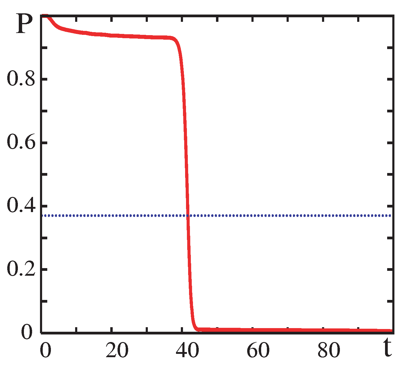
To demonstrate the influence of thermal effects, we studied first the absorption of the electron of a solectron in a cold lattice (
Figure 6) by following the electron probability density and the total probability (
Figure 7)
We observe that the solectron reaches the absorbing boundary at time , then the electron is absorbed almost entirely. Note that this corresponds in our model to the “time of arrival at the acceptor” or, in other words, as the “transition time donor-acceptor”. Note also that within the model a very small “part” of the electron probability density penetrates across the barrier. That the soliton keeps on moving is a specific feature of our model and may even increase its velocity when loosing its electron in the absorbing barrier. (Parameter values for the simulation are , , , , ). Next, we considered the heated lattice with the same parameter values for several temperature values. Initially, the electron is supposed to be localized (in the form of the Gaussian function) in the center of the chain.
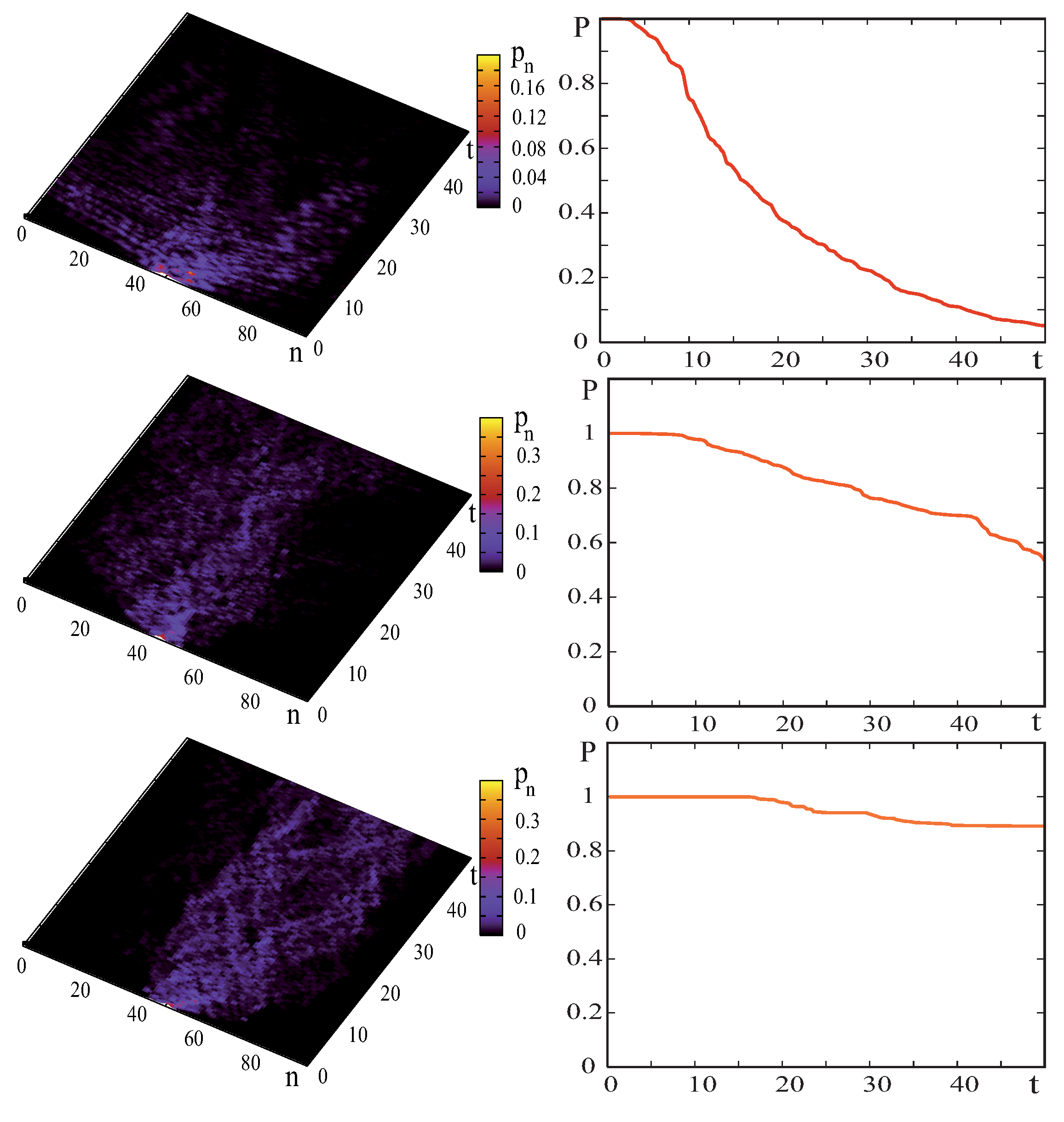
The results presented in
Figure 8 are based so far on one computer simulation for each temperature. Those figures show typical distributions of probability
(to find an electron at site “n”, the local electron density, left) and the total density P(t) (right). However, in order to estimate the transition time in a more correct way, we have to perform a set of computer simulations with different realizations of noise influence and then calculate an average characteristic value (
Figure 9).
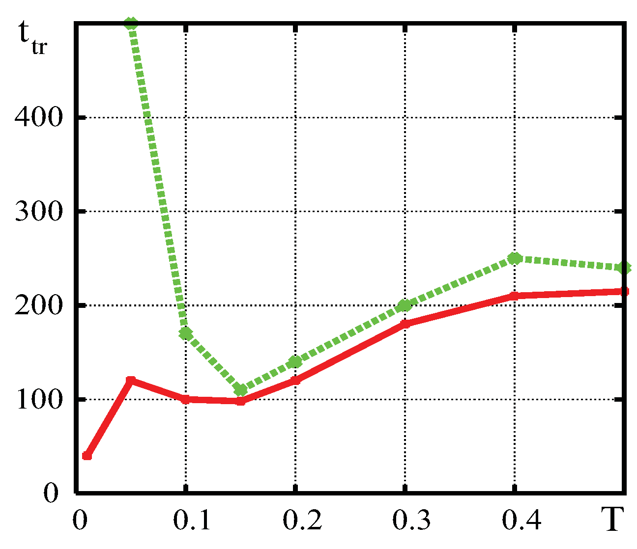
The averaged transition time as a function of temperature is presented in
Figure 10. The transition time is defined as a time when the total probability to fix an electron in a lattice becomes less than
(note that sometimes authors use as criterium “1/3” instead of 1/e). One may see that there is a minimum at temperature
, corresponding to the most effective interaction of the electron with solitons. Note that the transiton time is here a sum of two time intervals: first, the time to extract an electron from an “electron” potential well and, second, the travelling time of an electron along the lattice from the donor to the acceptor. Note also that the tunneling does not “work” at such long distances
, as the tunneling time is practically infinite [
13,
14]. In the case studied here, thermal transitions interfering with quantum effects dominate. The large values of the transition time
at low temperatures observed in
Figure 10 are to be explained by the fact that the first time interval grows sharply with temperature decreasing, although the electron travels along a lattice quickly. In contrast, at high temperature the electron is extracted from a well rapidly, but thermal solectrons become less stable.
To exclude the influence of characteristics of an initial potential well and exclude the contribution of “extracting” time to the transition time, a set of computer simulations have been performed for the initial state of an electron in the form of a narrow localized Gaussian bell in a non-deformed lattice consisting only of an absorber at the same position (
Figure 10). These results were obtained with a stochastic algorithm solver of master equations.
The results shown in
Figure 9 and
Figure 10 agree for high enough temperatures
but disagree somehow for lower temperatures
. This is due to the different behavior of the diffusion coefficient obtained in both formalisms (the purely quantum-mechanical and the quantum-statistical). In some sense, these two curves (
Figure 10) remind the two curves presented in
Figure 5; however, the details and the deeper reasons still remain unexplained. We have to take into account that the quantum mechanical diffusion (dispersion of the density) is not a physical diffusion process but just dispersion of wave functions. Our results strictly speaking are reliable only for
.
7. Discussion of the ET Donor-Absorber and the Transition Times
At very low temperature
, an initially localized wave function of the electron spreads along the lattice and the total probability P(t) to find the electron along the chain decreases in time approximately like an exponential function of time. Note that (1 − P(t)) is the probability of absorption. At
(weak nonlinearity), the total electron density P(t) decreases much slower and does not look like an exponential function of time. At
, several steps in the dependence P(t) are observed. In this case, the electron originally localized is quickly transformed to several solectronic maxima; the steps in P(t) correspond to the absorption of these solectronic maxima. At
, several solitons are excited which are moving oppositely carrying parts of the electron probability density. The probability of existence decreases rather slowly, it takes a very long time before the absorption occurs, and the electron may overcome a quite a long distance before absorption, provided the acceptor is placed far enough from the donor. In our diffusion model, the process is considered as a diffusion-controlled reaction. In the framework of the the Smoluchowski theory, the reaction rate of an electron with density
and one absorber with radius
at a fixed position is given by
We see that the rates are proportional to the diffusion coefficient of the electron,
. The electron probability density is decreasing with the distance and develops in time according to the diffusion law Equation (
12).
According to our estimate of the diffusion constant, reaction rates based on diffusion would first increase with temperature, then reach a maximum at
and then decay. The optimal temperature is somewhere around
in units of 2D. At this time, we are not aware of data which are in agreement with this prediction. Most data seem to show an exponential relation between distance and time. This point to the existence of other mechanisms for ET, such as tunneling [
4,
13,
14,
47,
50,
51].
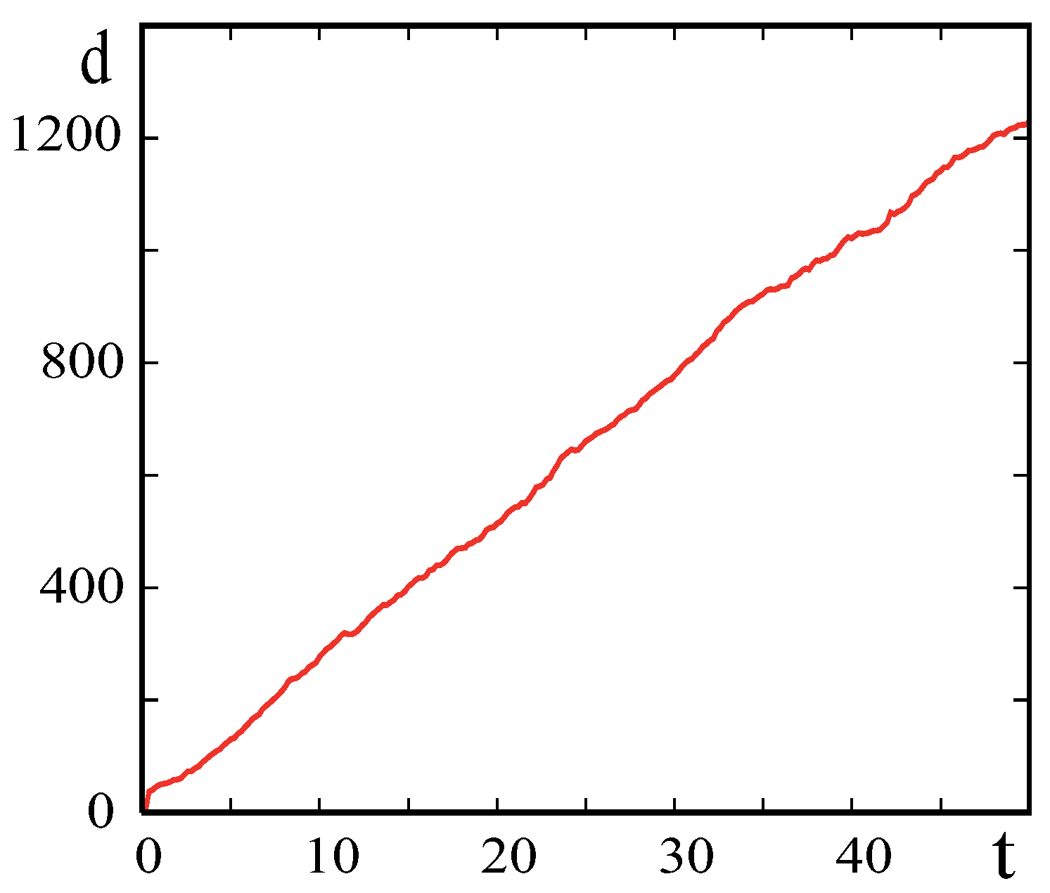
Nevertheless, let us try to give some estimates based on the two mechanisms studied here: surfing on external solitons and diffusion-like transport on thermal solitons.
Different computer simulations with absorbing boundary have been shown in
Figure 9. As shown by Chandrasekhar, diffusion transport is based on the mean square displacement which is given by Equation (
13) [
49]. He estimated the mean flow through an absorbing boundary located at
and found
Introducing here a dimensionless time
τ, we get
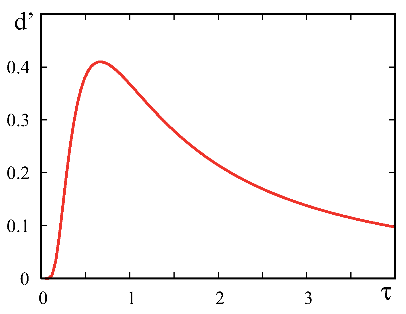
We show the flow d’ as a function of time according to the Chandrasekhar model in
Figure 11.
As
Figure 11 shows, the overwhelming amount of probability is absorbed within the (dimensionless) time
By returning to quantities with dimensions as Å and picoseconds,
This corresponds just to the mean square displacement which is
For the dimensionless effective diffusion coefficient
, we estimated a value around 30 close to to the maximum with respect to the temperature. This way, we estimate in dimensional quantities a value around 80 Å
/ps and, correspondingly, we find
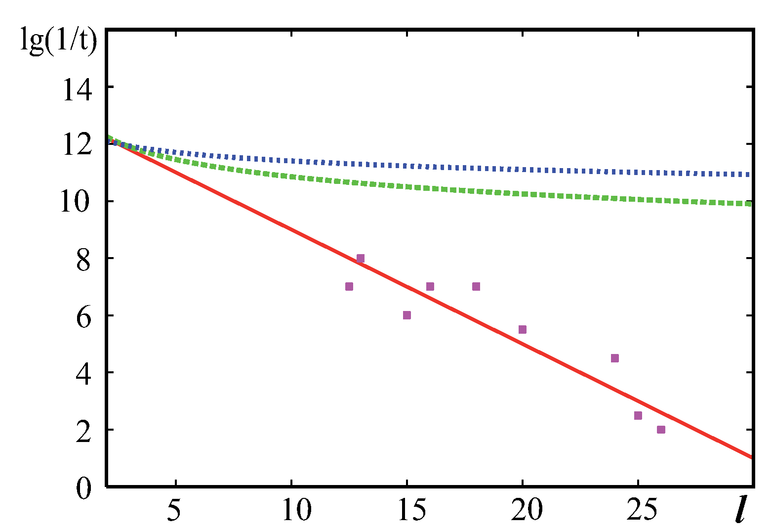
The empirical data are usually given as a log of the reciprocal time over the traveled distance given in Å [
18]. In our case, we get for the log of the reciprocal time the electron needs to travel the distance
the following estimate
This estimate in
Figure 12 is shown by the green curve (time is measured in seconds and the distance in Å, so the 12 (ordinate) corresponds to a picosecond, the six to a microsecond).
The estimate based on the diffusion mechanism is surely only a first rough result; in detail, things might be more complicated. Indeed, ET is more complicated than the simple diffusion-controlled reaction studied by Smoluchowski and Chandrasekhar [
48,
49]. Let us consider now the other mechanism of surfing on one externally excited soliton such that the electron will travel approximately with sound velocity from the donor to the acceptors:
. We estimate the sound velocity
c here as approximately 20 Å/ps. Let us mention that in some experimental work [
52] a sound velocity of 16.9 Å/ps was measured for DNA. We have
This is the blue curve we have drawn in
Figure 12. We see that the soliton-assisted mechanism (blue curve), which we discussed here is much faster than the estimated average of the observed data given by the lowest (red) curve where slower processes not yet understood seem to dominate in the overall balance.
8. Conclusions
We studied here several mechanisms of electron transfer in nonlinear lattices. We have shown that soliton-assisted electron transfer is one possible rather fast mechanism in a heated nonlinear lattice. We modeled the lattice dynamics with Morse interactions and the electron dynamics as well as the electron-lattice interaction in the quantum mechanical “tight binding” approximation. We have shown that, while the thermal solitons which comprise around 10 lattice sites provide the carrier, the electron “localization” on the lattice, strongly affects the ET-dynamics. The general tendency is that, due to this mechanism, the transfer is much slower and the living times of the solectrons are much higher than previously expected. A similar conclusion has been made based on a completely different method [
53]. These authors conclude, that “electronic coupling is most likely determined by nonequilibrium geometries beyond a critical distance (6–7 Å in proteins and 2–3 Å in water)”. In our work, some kind of “nonequilibrium geometries” are identified as local deformations due to thermal lattice soliton excitations.
In conclusion, regarding the role of solitons, we may say that electron surfing on lattice solitons generated by external sources provides an extremely fast way of ET (see the blue curve in
Figure 12); however, in this case, the source of solitons is yet to be identified. A possible candidate for the source for externally excited solitons are Volkenstein’s conformons [
54,
55,
56]. An alternative way of ET studied here, which is more natural, is the surfing on thermal solitons. The latter provides a slower transport mechanism, due to the quick change of thermal soliton directions. However, this surf is free since thermal solitons are always present. Note that this is a significant improvement relative to the less realistic model used in [
11]. A second mechanism, which is slower but still rather fast, is diffusion-based on thermal solitons (green curve in
Figure 12). We estimated here the needed times for donor-acceptor transitions based on the Smoluchowski–Chandrasekhar model of absorbing boundaries. The comparison with times observed in experiments (see lowest curve and data points in
Figure 12) shows that, under realistic conditions, the transition times are much longer, which means, in reality, the transitions are slowed down by other yet unknown mechanisms such as capturing by impurities. Indeed, as noted by Giese [
4] and others, the question of how electrons migrate over long distances was raised about thirty years ago and still is a matter of debate. One may assume that, in reality, one has a combination of several mechanisms, between them the very slow mechanism of tunneling may play quite a significant role [
4,
13,
14,
38,
39,
40,
47].
In conclusion, the computer simulations based on our simple models show that the real processes of donor-acceptor transitions may be very complex. It is to be understood with the interplay of several components such as tunneling, thermal activation, diffusion, electron surfing on lattice solitons and other effects. Clearly, the soliton-assisted transport is the fastest of them all eventually allowing the longest path (or shortest time). All this illustrates the rather difficult problem of dissipative quantum transport [
47].


