A Comparison of Classification Methods for Telediagnosis of Parkinson’s Disease

Abstract

Parkinson’s disease (PD) is a progressive and chronic nervous system disease that impairs the ability of speech, gait, and complex muscle-and-nerve actions. Early diagnosis of PD is quite important for alleviating the symptoms. Cost effective and convenient telemedicine technology helps to distinguish the patients with PD from healthy people using variations of dysphonia, gait or motor skills. In this study, a novel telemedicine technology was developed to detect PD remotely using dysphonia features. Feature transformation and several machine learning (ML) methods with 2-, 5- and 10-fold cross-validations were implemented on the vocal features. It was observed that the combination of principal component analysis (PCA) as a feature transformation (FT) and k-nearest neighbor (k-NN) as a classifier with 10-fold cross-validation has the best accuracy as 99.1%. All ML processes were applied to the prerecorded PD dataset using a newly created program named ParkDet 2.0. Additionally, the blind test interface was created on the ParkDet so that users could detect new patients with PD in future. Clinicians or medical technicians, without any knowledge of ML, will be able to use the blind test interface to detect PD at a clinic or remote location utilizing internet as a telemedicine application.

1. Introduction

New telecommunication technologies are increasingly being applied to healthcare resulting in better health outcomes. Telemedicine allows rapid and accurate detection of certain diseases. Computer-aided diagnosis has become common [1,2,3,4,5]. ML [6,7] and telemedicine has been implemented in diagnosis of diseases in several therapeutic areas including cardiology [8], chest disease [9], radiology [10], pathology [11], neurology [12], pediatrics [13], dermatology [14], and psychiatry [15]. Additionally cellphone, image sensor or Google Glass-based medical devices have been adapted for telemedicine and point of care applications [16,17,18,19,20,21].

Parkinson’s disease is a neurodegenerative disorder that has significant adverse effect on the lives of patients and their families [22,23,24]. Early and accurate diagnosis of PD is critical for effective treatment, but unfortunately PD diagnosis is not efficient. Computer-based smart systems can detect PD symptoms. Wavelet transformation through web interface was used to detect the difference between spirals drawn by PD patients and healthy participants using an ergonomic pen on a hand computer [25]. An automatic characterization of PD was developed by measuring the ipsilateral coordination and spatiotemporal gait patterns and using SVM [26]. Vegetative locomotor coordination, with an automatic step detection component and template matching algorithm, was used for the analysis of patients with PD [27].

Little et al. measured dysphonia from patients with PD [28]. They recorded an average of six phonations from each patient. A soundproof audiology booth produced by an industrial acoustics company was used to record the phonations by utilizing a microphone which is mounted on the head. Using a computerized speech laboratory, the human sound signals were recorded on a computer. After recording the phonations, they calculated the existing traditional and nonstandard measures and entropy of some variations. They discriminated healthy people and patients with PD using a kernel SVM classifier. Some researchers subsequently used Little et al.’s dataset and tried to improve the performance of their classifier. Bhattacharya et al. used the data mining tool Weka and SVM as classifiers [29]. Das tried to select features and applied four different classifiers including neural networks, DMneural, Regression and decision tree [30]. Sakar et al. also applied a feature selection method and used a SVM classification algorithm [31]. Ozcift selected the features with linear SVM then, applied IBk (a k-Nearest Neighbor variant) classifier [32]. Polat classified patients with PD using a feature weighting method named fuzzy c-means clustering-based feature weighting (FCMFW) and k-NN classifier [33]. Acevedo used an alpha-beta bidirectional associative memory (ABBAM) approach to differentiate between patients with PD and healthy people [34]. Gök selected features and used six different classifiers: Bayes net, linear SVM, radial basis SVM, k-NN, multilayer perceptron, and K-Star [35].

In this study, the PD dataset produced by Little et al. was used and a novel method for detection of PD was developed in a different way as compared to previous studies. A new program named the ParkDet 2.0 was created by using a MATLAB graphical user interface (GUI) to implement the ML process on the program. Then, using the ParkDet, different combinations of ML were applied to increase the accuracy of classifier. The principal purpose of the study is to allow clinicians or medical technicians to detect patients with PD utilizing the easy-to-use ParkDet program and not to require them to use complex engineering programs such as MATLAB and automatic detection methods. Through the ParkDet program several combinations of ML processes were applied such as PCA and factor analysis (FA) as FT, and seven classifiers such as Support Vector Machine (SVM), Boosting, k-NN, Naive Bayes (NB), Decision Tree (DT), Linear Discriminant Analysis (LDA) and Quadratic Discriminant Analysis (QDA) with 2-, 5- and 10-fold cross-validations and an additional blind test. The results are encouraging since the accuracy of classification reached 99.1%, which is the highest one reported compared to other techniques in the current literature.

2. Materials and Methods

2.1. Dataset

The dataset comprised 195 sustained vowel vocalizations from 31 people of which 23 have been diagnosed with PD. Nineteen of the 31 people are male and the rest are female. The dataset includes 195 phonations of participants consisting of 48 healthy and 147 diagnosed with PD. A microphone was mounted on the participant’s heads and the phonations were recorded. An average of six phonations was recorded from each candidate. The software Praat 4.3.14 [28,36] and Kay Pentax multidimensional voice program (MDVP), model 4337, [28,37] were used to calculate the traditional measures. Using a computerized speech laboratory, the voice signals were recorded on a computer. The dataset has 22 dimensional features as given in

Table 1. The 22 features and short definitions of the original PD dataset.

Features	Definitions
MDVP: Fo (Hz)	Average vocal fundamental frequency
MDVP: Fhi (Hz)	Max. vocal fundamental frequency
MDVP: Flo (Hz)	Min. vocal fundamental frequency
MDVP: Jitter (%)	Jitter as a percentage
MDVP: Jitter (Abs)	Absolute jitter in microseconds
MDVP: RAP	Relative amplitude perturbation
MDVP: PPQ	Five-point period perturbation quotient
MDVP: Shimmer	local shimmer
MDVP: Shimmer (dB)	local shimmer in decibels
MDVP: APQ	11-point amplitude perturbation quotient
Shimmer: APQ3	Three point amplitude perturbation quotient
Shimmer: DDA	Average absolute difference between consecutive differences between the amplitudes of consecutive periods
Shimmer: APQ5	Five point amplitude perturbation quotient
Jitter:DDP	Average absolute difference of differences between cycles, divided by the average period
NHR	Noise-to-harmonics ratio
HNR	Harmonics-to-noise ratio
RPDE	Recurrence period density entropy
DFA	Signal fractal scaling exponent
D2	Correlation dimension
PPE	Pitch period entropy
Spread1	Two nonlinear measures of fundamental frequency variation
Spread2

with their short definitions. The patients’ ages ranged from 46 to 85. The mean and standard deviation of the ages are 65.8 and 9.8, respectively. The dataset was recorded at the University of Oxford, in collaboration with the National Centre for Voice and Speech (Denver, CO, USA) and shared online in the UCI machine-learning archive [28].

Little et al. [28] demonstrated a practical assessment of existing traditional and nonstandard measures of dysphonia in the literature and additionally, they measured a new variation of dysphonia. They acquired pitch pattern of the vocalization and converted it to a logarithmic halftone measure and then built a discrete probability distribution of generation of relative halftone alteration. They then computed the entropy of this probability distribution. They denominated the new variation as pitch period entropy (PPE).

Entropy is used to calculate quantification of the uncertainness of a random variable X. Namely, the entropy quantifies -the difficulty of variable prediction. The mathematical expression of Shannon’s entropy is given by:

$$\mathit{H}\left(\mathit{X}\right)=-{\displaystyle \sum }_{\mathit{x}}\left[\mathit{p}\left(\mathit{x}\right)\log \left(\mathit{p}\left(\mathit{x}\right)\right)\right]$$

(1)

where p(x) is the probability distribution function belonging X. The unevenness of the probability distribution p is quantified by Equation (1) [38].

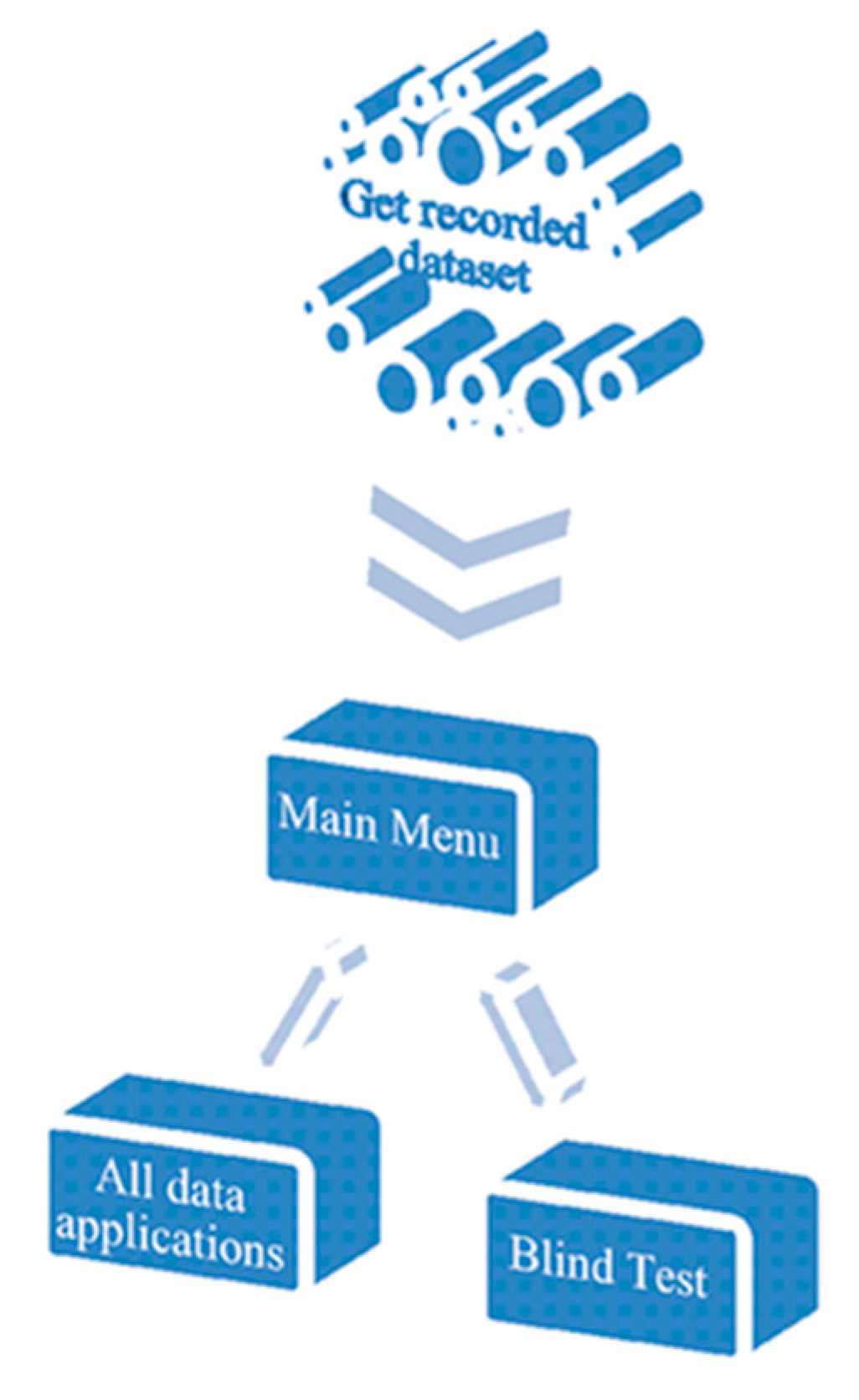
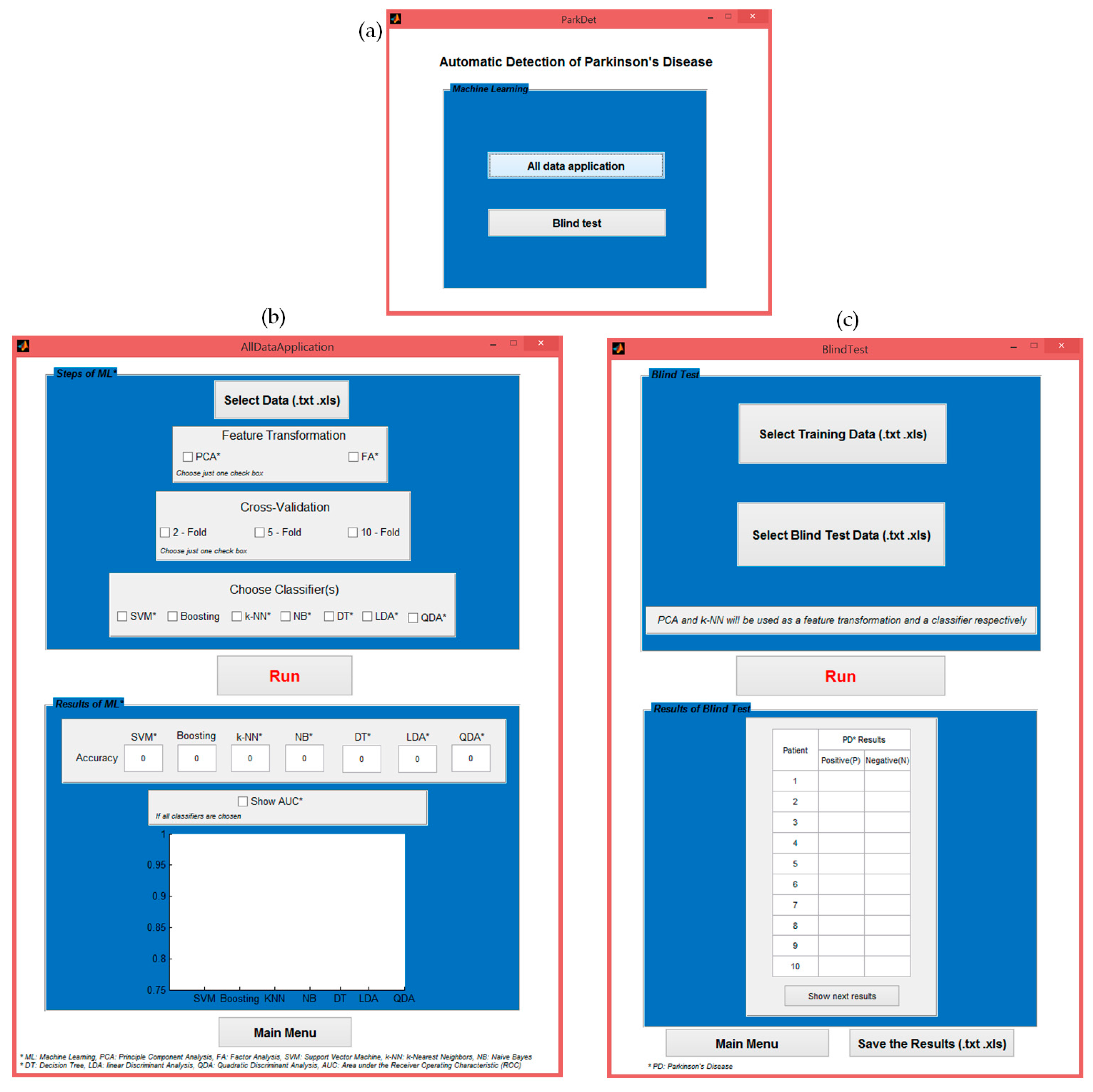
2.2. Telemedicine Application with the Created ParkDet 2.0

A new program called ParkDet was created to apply multiple ML algorithms to the dataset of prerecorded PD. Interfaces of the program, created in MATLAB GUI, were transformed to a user friendly program. The interfaces consist of three pages called “Main menu”, “All data application” and “Blind test”. The relationship between these interfaces is shown as Figure 1. Prerecorded dataset can be accessed through internet or USB memory, and then ML processes can be applied, using ParkDet, to distinguish patients with PD from healthy people. ParkDet was employed by installing it on a Windows-based tablet. When the program is run, the main menu interface is seen (Figure 2a), and users can switch to the other screens through the pushbuttons.

On the main screen there are two buttons named “All data application” and “Blind test”. In the meantime, users can return to the main menu screen from the other screens, using “Main Menu” pushbutton at the bottom of the all data application and blind test screens. When a user pushes the “All data application” button on the main menu interface, the screen shown in Figure 2b is seen. All data application interface consists of two sections called “Steps of ML”, “Results of ML” and also, “Run” and “Main Menu” buttons. The interface is designed as a flow chart to enable user-friendly use. Users will be able to use the ParkDet by starting from the top of the interface proceeding to the bottom. At the “Steps of ML” section, there are four sub-steps to apply ML process: 1. Select data. 2. The feature transformation methods. 3. The numbers of k-fold for cross-validation. 4. The classifier(s).

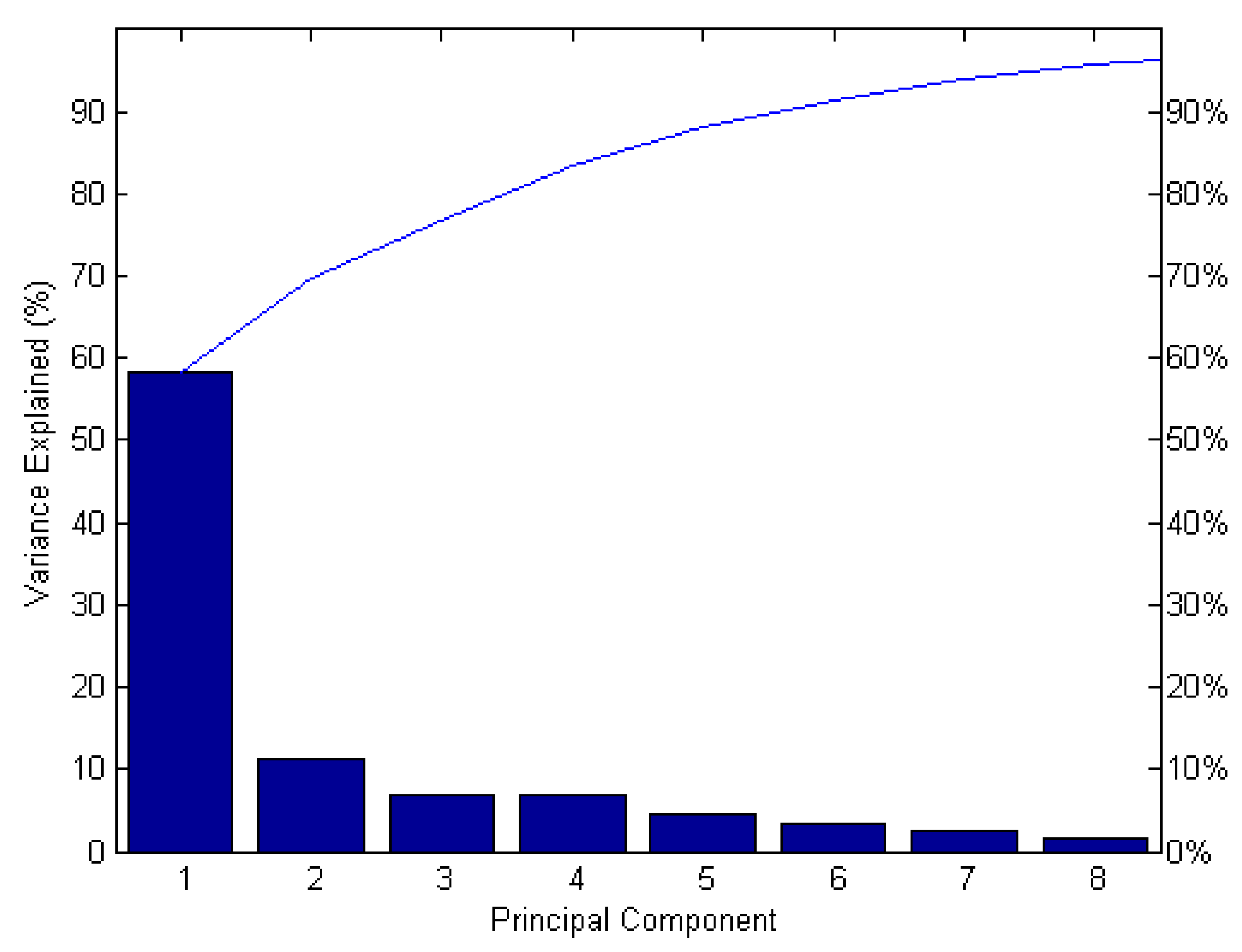
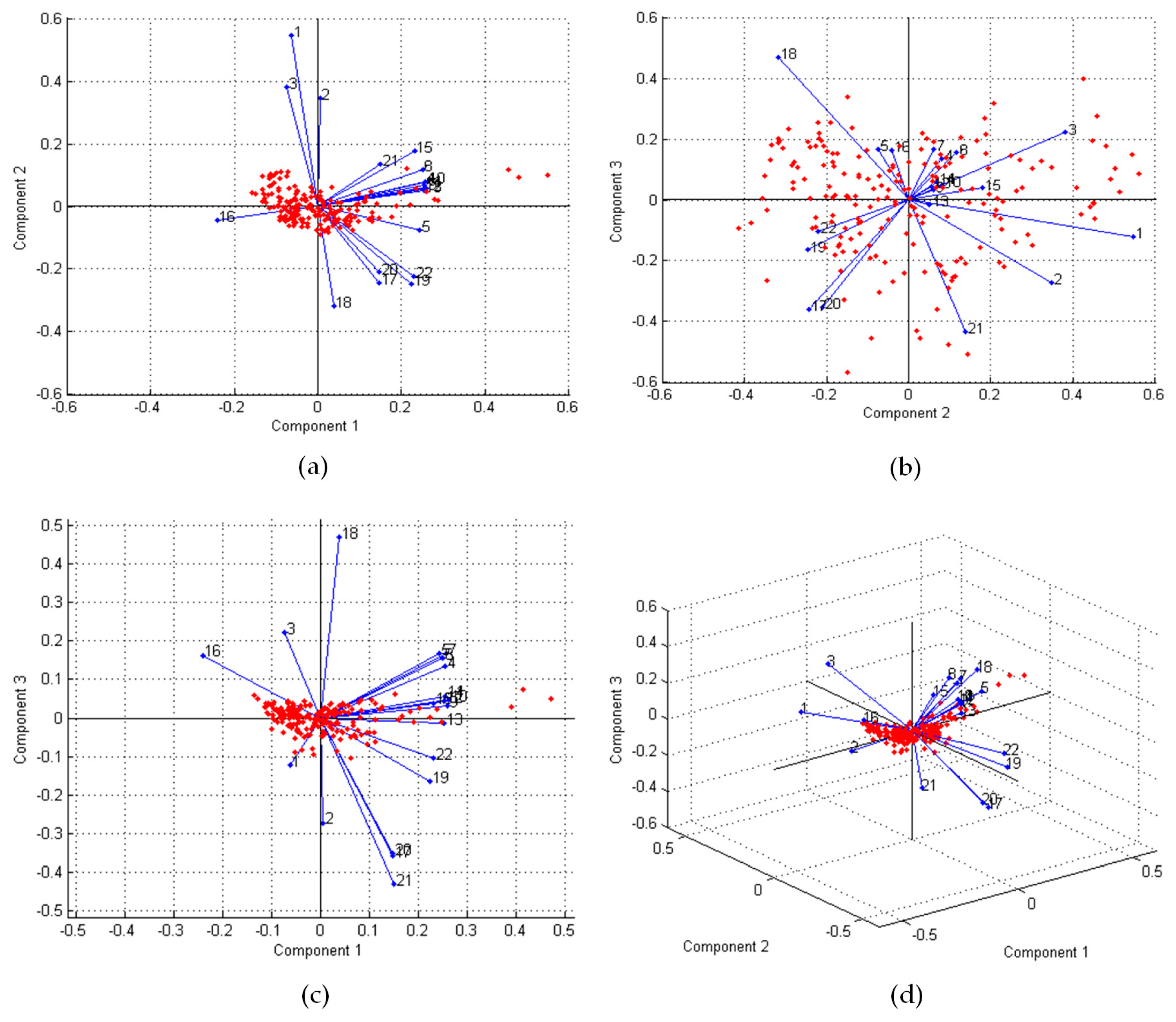
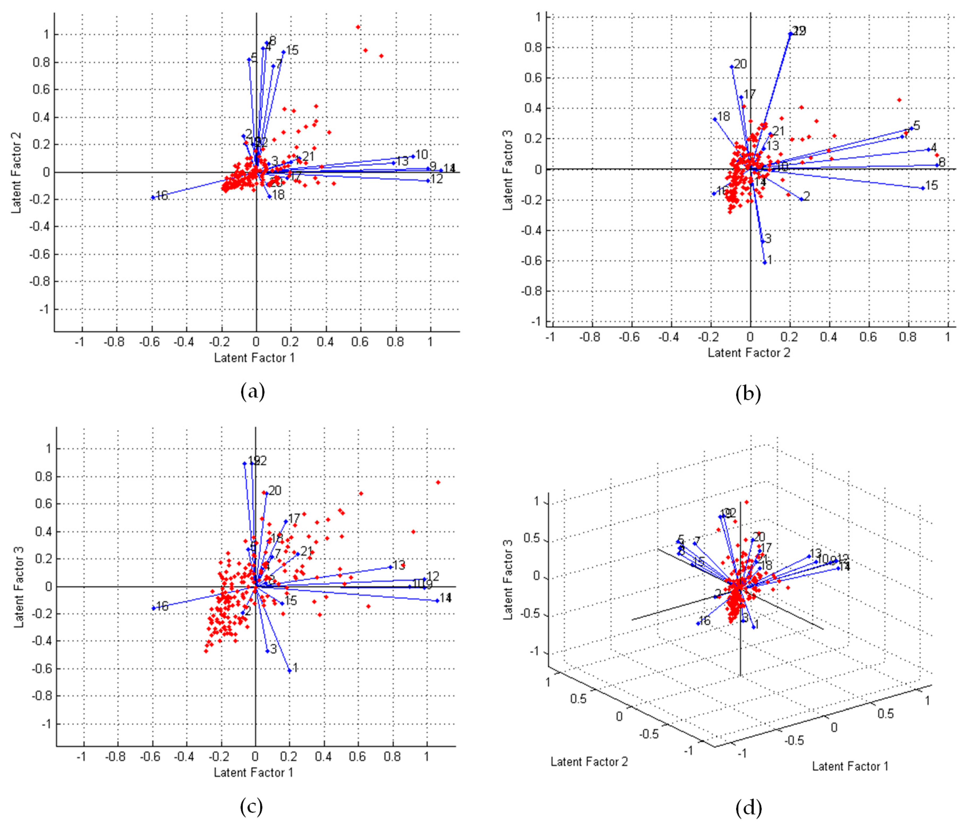
2.2.1. Feature Transformation

The user selects the prerecorded dataset in the tablet and PCA or FA can be chosen as a FT method. FT is useful for dimension reduction of features and creates new predictor features. FT is practiced on the PD dataset by creating new reduced features that represent information entropy of the original dataset. Principal Component Analysis (PCA) is a statistical method to transform variations from probably correlated features of the observations to the uncorrelated features called principal components. One of the utilization areas of PCA is reducing variations to create predictive new features [39]. Factor analysis is a statistical approach and a useful method to eliminate redundant of features. FA redesigns the features as linear combinations of the potential factors [40].

2.2.2. Cross-Validation

K-fold is created in the cross-validation. K-equal sized subsamples are created from the original samples. In this study, 2-, 5- and 10-fold can be selected using check boxes in the ParkDet interface. Test data is created using a single subsample of the k subsamples and the rest of subsamples constitute the training data. Throughout each of k times repetition of cross-validation procedure, individual k subsamples are used as the test data. To achieve a single prediction, k accuracy results, which are obtained from the all folds, of implemented classifiers in this study were averaged [41].

2.2.3. Classification Algorithms

Users can elect to apply SVM, boosting, k-NN, NB, DT, LDA or QDA as the classifiers using check box(es). The maximum margin hyperplane, which is defined by the SVM, is used for the purpose of differentiating between two classes of patterns. Margin means the width of the slab parallel to the hyperplane which has no interior data points [42]. In this study, radial basis SVM was used. Boosting reduces bias primarily and also variance as a machine learning ensemble meta-algorithm, the aim of boosting is to convert weak learners to strong ones [43]. There are many boosting algorithms. In this study the adaptive boosting (AdaBoost) algorithm was used. The k-NN classification is one of the most fundamental and simple classification methods and finds a group of k that is the number of nearest neighbor objects which are closest to the test object. The number of nearest neighbors, labeled objects and similarity measurements to calculate distance between the value of k, and objects, are significant parameters to gain high accuracy of k-NN. The distance between unlabeled objects and labeled object is calculated to determine the classes of unlabeled objects. After identifying the k-nearest neighbors, the class label of the objects are achieved by using the class labels of the k-nearest neighbors [44]. The Naive Bayesian classifier, which is based on Bayes Theorem, is simply realizable and includes no complexity of iterative parameter estimation which makes it ideal to use for sizeable datasets [45]. A decision tree is a prevalent method for decision analysis and classification in machine learning and comprises a root and a number of nodes, branches representing conjunctions of features and leaves representing class labels and the elements of decision tree constitute a tree-shaped schematic representation. Classification process is realized by starting at the root of the tree and proceeded to a leaf node [46]. Linear and quadratic discriminant analysis acquires a hyperplane to separate two classes. This method is based on the mean and pooled matrix of the data. It must be that all variables have a normal distribution. In the meantime, for all groups, the variance and covariance of matrix must be homogeneous to practice the discriminant analysis. QDA and LDA are similar methods. However, QDA of a covariance matrix must be predicted for each class as differently [47,48].

The “Results of ML” section has two sub-steps. After the check boxes of the ML steps are selected, if a user pushes the “Run” pushbutton, the accuracies of all classifiers instantaneously appear at the first step of the Results in the ML section. At the same time, the area under the Receiver Operating Characteristic (ROC) curve (AUC) can be seen at the second step of the Results of ML section if a user selects all classifiers and clicks the “Show AUC” check box. To plot ROC curves, true positive and false positive rates with different threshold values are used. By utilizing the area under the ROC curve, an AUC value is calculated and plotted. The AUC value is accepted to be a significant benchmark of comparison for performances of classification algorithms [49]. After all processes are finished, the user can close the program or go back to the main menu by pushing the “Main Menu” button.

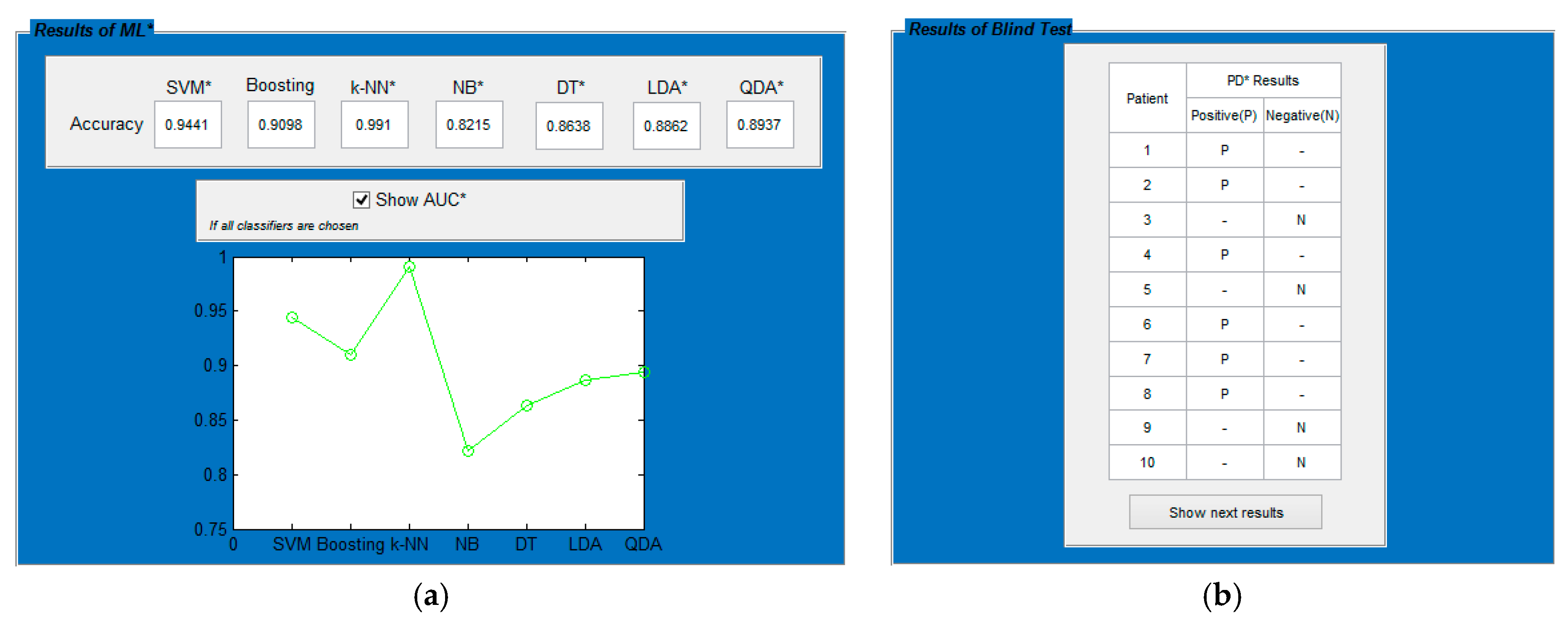
2.2.4. Experimental Implementations

Using the “All data application” interface of the ParkDet, the prerecorded dataset was selected and several ML combinations were applied. The original dataset without FT, 2-fold cross-validation and all classifiers were chosen and the program was run. Accuracies of results were saved and AUC was observed for comparison of classifications. This process was repeated choosing 5- and 10-fold cross-validation for original dataset and accuracies of all classifiers were saved.

After these three processes, PCA was applied to the dataset and feature reduction was performed. The relationship between random variables is observed with multivariate statistics. A multivariate data matrix of X is the set of observations of the random variables. The sample mean of the kth variable is as Equation (2):

$${\overline{\mathit{x}}}_{\mathit{k}}= \frac{1}{\mathit{n}}{\displaystyle \sum }_{\mathit{i}=1}^{\mathit{n}}{\mathit{x}}_{\mathit{i}\mathit{k} }, \mathit{k}=1,2,\dots ,22$$

(2)

where, k and n are the number of variations and observations respectively. The variance is defined by Equation (3) and covariance is calculated with Equation (4):

$${\sigma }_{\mathit{k}}{}^2= \frac{1}{\mathit{n}} {\displaystyle \sum }_{\mathit{i}=1}^{\mathit{n}}{\left({\mathit{x}}_{\mathit{i}\mathit{k}}-{\overline{\mathit{x}}}_{\mathit{k}}\right)}^2 , \mathit{k}=1,2,\dots ,22$$

(3)

$${\mathit{C}}_{\mathit{i}\mathit{k}= }\frac{1}{\mathit{n}} {\displaystyle \sum }_{\mathit{j}=1}^{\mathit{n}}\left({\mathit{x}}_{\mathit{j}\mathit{i}}-{\overline{\mathit{x}}}_{\mathit{i}}\right)\left({\mathit{x}}_{\mathit{j}\mathit{k}}-{\overline{\mathit{x}}}_{\mathit{k}}\right) , \mathit{i}=1,2,\dots ,22, \mathit{k}=1,2,\dots ,22$$

(4)

Figure 3 shows the total variance of the first eight components (instead of the total twenty two) as 95.68%.

First principal component (PC) possesses the biggest variance. Using PCA, 22 features were now reduced by eight principal components. When the new reduced features are used, only 4.32% of information is excluded since the total variance is 95.68%. Through PCA, the original data can be easily visualized. After reducing the data dimensions, a visual representation of the data is observed. The comparison of samples and variables for PC1 versus PC2, PC2 versus PC3, PC1 versus PC3 and PC1 versus PC2 versus PC3 as 3D are shown in Figure 4a–d, respectively.

All twenty two variables are represented by a vector in Figure 4. The contribution of each variable to the two or three principal components can be seen by the direction and magnitude of that vector. Each blue line represents the 22 corresponding features as labeled. The significance of that feature can be observed with the magnitude of the associated line. The most significant variable having the largest negative coefficient for PC1 is 16th variable corresponding to the HNR since the location of variable is far from origin. 1st variable MDVP Fo(Hz) is the most significant feature for PC2 and 18th feature DFA is the most significant variable for PC3 having the largest positive coefficients. Figure 4d as 3D image provides a good comparison of significant variables. 1st, 2nd, 3rd, 16th, 17th, 19th, 20th, 21st, 22nd variables as MDVP Fo(Hz), MDVP Fhi(Hz), MDVP Flo(Hz), HNR, RPDE, D2, PPE, Spread1, Spread2 are more significant separator than the other ones. When the 3D figure is viewed from other angles in Figure 4d, the 18th variable’s DFA is clearly seen to be a significant feature. Using the new predictor features achieved via PCA, all classifiers with 2-, 5-, 10-fold cross-validation were chosen on the ParkDet, respectively. For these new three processes, all accuracies of classifiers were saved and the AUC was analyzed for comparison of the classifiers.

After analyzing the original dataset and the reduced dataset with PCA, the new transformed dataset was created by applying factor analysis technique. Three principal factors are extracted from the PD dataset. The covariance matrix of the dataset is calculated via Equation (5):

$${{\displaystyle \sum }}^{\text{}}= \mathit{\Lambda }{\mathit{\Lambda }}^{\mathit{T}}+ \mathit{\Psi }$$

(5)

where Λ is the matrix of loadings that are coefficients, and Ψ is the specific variances. Each column of Λ is a factor. The estimated loadings and the estimated specific variances provide to analyze the variables. When the non-rotated factors are observed, the factors representation is found to be difficult to interpret. The factors are then rotated to find a solution of the representation problem. Factor rotation provides to compute new loadings in the rotated factor coordinate system to fit the variations on the factor axis. After rotating the factors, the visual representation of the fitted data is observed by plotting the latent factors (LF). In Figure 5a–d LF1 versus LF2, LF2 versus LF3, LF1 versus LF3 and LF1 versus LF2 versus LF3 as 3D are shown.

The magnitude and direction of the vectors line indicate how each variable depends on the factors. Especially, it is observed that the 9th, 10th, 12th 13th, 14th variations have positive, 16th has negative loadings on the LF1 and 4th, 5th, 6th, 15th features have positive loadings on the LF2. 19th, 20th, 22nd have positive, 1st, 3rd have negative loadings on the LF3. Rests are around the origin. Using these new reduced predictor features via FA, all processes were repeated one more time and all accuracies of the classifiers with 2-, 5-, and 10-fold cross-validation were saved observing AUC to compare the classifications.

2.2.5. Blind Test Implementation

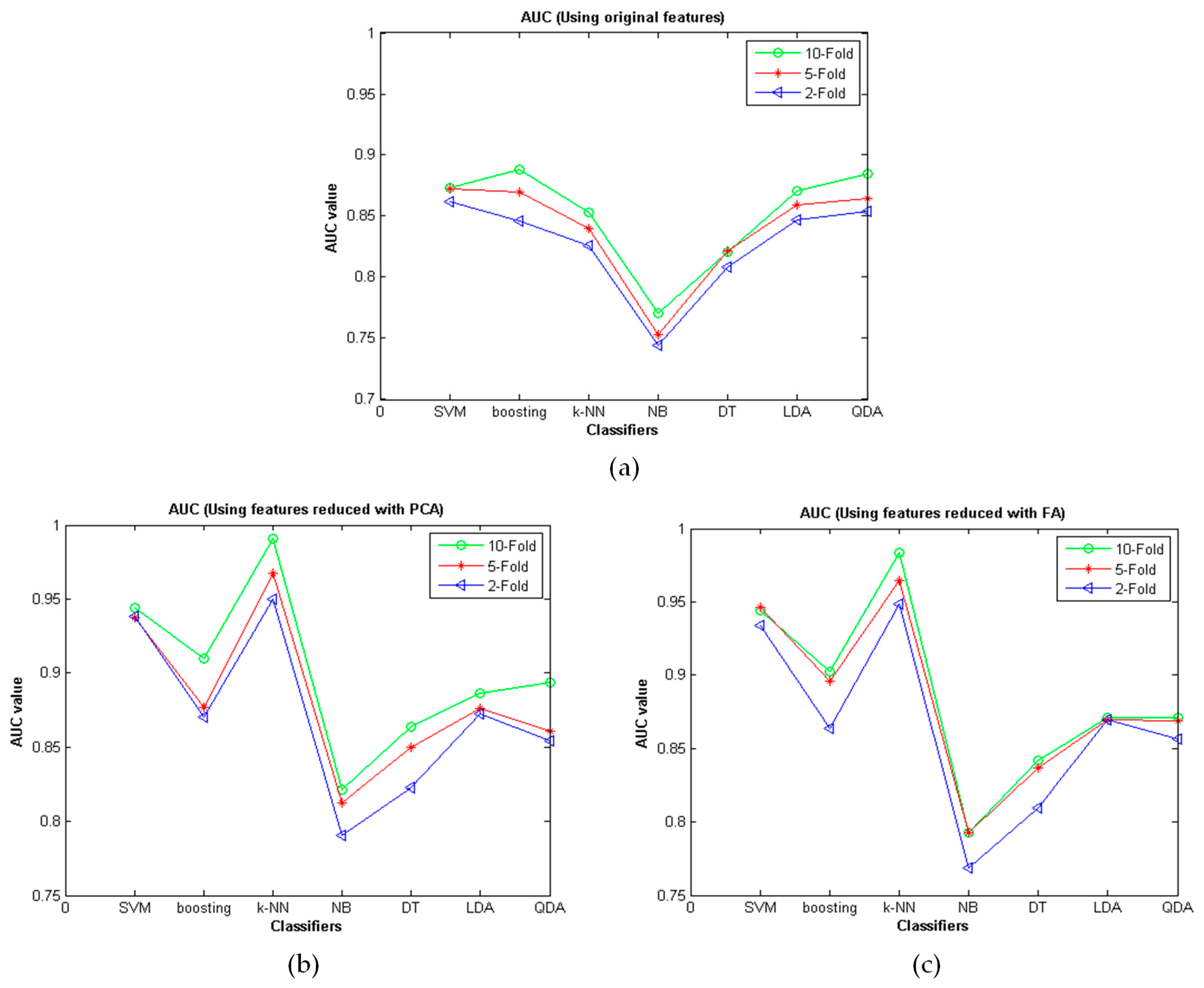
When users push the blind test button on the main menu interface, Figure 2c will be displayed. The blind test interface consists of two sections, named “Blind Test” and “Results of Blind Test”, in addition to, a “Run”, “Main Menu” and “Save the Results” buttons. In the blind test section, there are two pushbuttons. Using the first button, training data predetermined as the best is selected. Using the second button, test data is selected. When a user pushes the “Run” button, the results of ten patients can be seen as positive or negative in the “Results of Blind Test” section. For results of more than 10 patients, the user has to push “Show next results” button. The table was designed and limited to show ten patients because of screen size. However a user can process data for many more than ten patients and save the positive or negative results as a table in an Excel worksheet or notepad file.

In the all data application section the best training data was determined. The data with PCA and k-NN classifier with 10-fold cross-validation yielded the best accuracy. Cross-validation creates 10 different folds and uses all of them sequentially as a test dataset. Their obtained average accuracy is reported at 99.1% as the highest accuracy in the literature up to now. For the 10 different test data, 10 different accuracies were examined and the highest one, which was observed as 100%, was chosen. In the loop which has the highest accuracy, 176 of 195 data was saved and selected as the best training data, the remaining 19 of 195 data were saved as test data. The blind test interface was then used. The saved best training and test data were selected using the pushbuttons separately and the program was run. The results of patients were observed as positive or negative with 100% accuracy and were saved as an excel sheet (Figure 6b). Using the mentioned blind test interface with the best training data, it is thought that new candidates of patient with PD can be examined in future.

3. Results

Using the created three interfaces of ParkDet program, different combinations of ML were applied. All classifiers with 2-, 5-, and 10-fold cross-validations were applied to the original dataset, and the dataset were transformed using PCA and FA sequentially. Nine different combinations of ML processes were implemented and all accuracies of all classifiers were saved. 2-Fold cross-validation allows 50% of dataset to be used for training and 50% for test data. 2-Fold cross-validation accuracies of the datasets that are original, with PCA and FA, can be seen at

Table 2. Accuracies of classifiers with 2-fold cross-validation.

Dataset	SVM	Boosting	k-NN	NB	DT	LDA	QDA
Original	0.8615	0.8462	0.8258	0.7446	0.8087	0.8465	0.8539
with FA	0.9338	0.8636	0.9487	0.7690	0.8097	0.8696	0.8563
with PCA	0.9385	0.8705	0.9502	0.7903	0.8227	0.8723	0.8539

. There are no significant improvements among the accuracies of classifiers in the original dataset and reduced dataset except SVM and k-NN classifier. There is a significant improvement with the k-NN classifier. The accuracy is obtained as 82.58% when original dataset is used, it is 94.87% when FA feature transformation is used and 95.02% when PCA is used.

5-Fold cross-validation allows 80% of the dataset to be used for training and 20% for test data. The accuracies of classifiers with 5-fold cross-validation can be seen in

Table 3. Accuracies of classifiers with 5-fold cross-validation.

Dataset	SVM	Boosting	k-NN	NB	DT	LDA	QDA
Original	0.8728	0.8697	0.8395	0.7534	0.8215	0.8592	0.8642
with FA	0.9461	0.8961	0.9649	0.7930	0.8365	0.8698	0.8686
with PCA	0.9376	0.8765	0.9672	0.8125	0.8497	0.8764	0.8608

. Similarly, there is no improvement at this step, except for SVM and k-NN which are the best ones. The dataset with PCA has a higher accuracy at 96.72% than both original dataset and the dataset with FA. In the same way, it has higher accuracy than those of 2-fold experiments.

10-Fold cross-validation allows the use of 90% of the dataset for training and a 10% test dataset. The accuracies of classifiers with 10-fold cross-validation can be seen in

Table 4. Accuracies of classifiers with 10-fold cross-validation.

Dataset	SVM	Boosting	k-NN	NB	DT	LDA	QDA
Original	0.8735	0.8882	0.8532	0.7702	0.8210	0.8710	0.8847
with FA	0.9439	0.9026	0.9832	0.7928	0.8417	0.8713	0.8712
with PCA	0.9441	0.9098	0.9910	0.8215	0.8638	0.8862	0.8937

. This experiment has a best accuracy of 99.1% using PCA, k-NN classifier with 10-fold cross-validation.

In this experiment, PCA, 10-fold cross-validation, all classifiers and “Show AUC” were chosen and the program was run. All classifier results can be observed on the first step of “Result of ML” section and at the same time the AUC plot can be seen to compare the accuracy results as shown in Figure 6a. Additionally, to see the difference between 2-, 5- and 10-fold cross-validation results, the AUCs were created as shown in Figure 7a–c using all classifiers via the original dataset, reduced dataset with PCA and FA, respectively.

When the Original PD dataset is used, achieved accuracy values of classifiers are less than 90% (Figure 7a). After feature reduction with both FA and PCA, it is observed that the accuracies of SVM and k-NN show a significant improvement. There are also slight accuracy improvements for boosting, NB, LDA and QDA after feature reduction, but the best one is k-NN. Additionally, Figure 7b,c enable comparison of the FA and PCA feature reduction methods with respect to the PD dataset. PCA gave the best reduced features and FA also gave good reduced features. Their performance is similar, but is not the same as they are related to each other but are not identical.

Using the best combinations of ML, the blind test interface was created. The best training data and test data were chosen from the experiment using PCA, k-NN with 10-fold cross-validation. The reported best accuracy, 99.1%, is the average of the results from 10-fold cross-validation. Some of the 10-fold results had 100% accuracy. One of them was chosen and its training and test datasets were saved as the best ones. Using the blind test interface, saved training and test data were selected and the program was run. The results of 10 patients were seen as positive or negative as shown in Figure 6b. There were 19 test data so, the next results of nine patients were observed by pushing “Show next results” button and the results were saved as a excel sheet having 100% accuracy by pushing “Save the Results”.

4. Discussions

A comparison of the accuracy of the method proposed in this study and the accuracy of the previous studies is provided in

Table 5. The comparison of the previous studies.

Reference	Classifier	Accuracy (%)
Developed method	k-NN using the created ParkDet 2.0	99.1
Little [28]	Kernel SVM	91.4
Battacharya [29]	SVM	65.22
Das [30]	Neural Network	92.9
Sakar [31]	SVM	92.75
Polat [33]	FCMFW	97.93
Acevedo [34]	ABBAM	97.17
Ozcift [32]	IBk	96.93
Gök [35]	k-NN	98.46

. Little et al. [28] recorded the voice of PD candidates and using kernel SVM, they distinguished the patients with PD from healthy people with 91.4% accuracy. Using their dataset, several researchers have tried to improve the accuracy of the ML classifier. Battacharya et al. [29] and Sakar et al. [31] have used SVM and achieved 65.22% and 92.75% accuracies, respectively, Das [30] achieved 92.9% accuracy using a neural network. Polat [33] tried a new method named fuzzy c-means clustering-based feature weighting and Acevedo et al. [34] tried an alpha-beta bidirectional associative memory approach and they reported the accuracies of their classifiers as 97.93% and 97.17%, respectively. Ozcift [32] applied the IBk (a k-Nearest Neighbor variant) method and attained 96.93% and Gök [35] used k-NN classifier and reached 98.46% accuracy. The accuracy of this study is the highest at 99.1% when 10-fold cross-validation was used with PCA. Using FA feature reduction technique with 10-fold cross-validation, 98.32% accuracy was achieved. This accuracy value is also greater than some other studies in the literature [28,29,30,31,32,33,34]. Moreover, when 2-fold cross validation with PCA and k-NN are implemented, it is observed that the accuracy at 95.02% is better than some studies [28,29,30,31]. The 2-fold cross-validation process uses 50% training and 50% test data. For ML, classifying the features with 50% training and 50% test data is more difficult than with 90% training and 10% test data achieved by using 10-fold cross-validation. When this condition is considered, the result of this study is better than the studies in the literature. Additionally, using the automatic detection program ParkDet via an easy-to-use blind test interface, clinicians or medical technicians can run ML without any codes to distinguish the patient with PD from the healthy people.

5. Conclusions

In this study, a novel telemedicine technology for automatic detection of PD was developed by creating a new program named ParkDet 2.0. The main goal of the ParkDet program is for clinicians or medical technicians (without knowing ML code) to easily apply ML processes, to distinguish patients with PD from healthy people using prerecorded voice features. In order to be a user friendly program, ParkDet was designed as a flow chart. The user proceeds through the program by starting from the top of the interface to the bottom sequentially. Using the ParkDet, several ML combinations were applied to the prerecorded PD dataset. The highest accuracy achieved was 99.1%. Additionally, via the blind test interface, new patients with PD can be distinguished from healthy people during real-time medical examinations as soon as the data is recorded at a clinic or remote location utilizing the internet as a telemedicine application. As a distinctive and novel application program ParkDet is an ongoing project for future improvements and updates. Two new interfaces can be added. One of them might provide that the voices of patients are recorded to the tablet directly. Another one can process regression methods to be analyzed gait or motor skill variations differently. It is thought that the developed automatic PD detection technique with created telemedicine application named ParkDet will help the clinicians to diagnose the patients with PD.

References

1. Calle-Alonso, F.; Pérez, C.J.; Arias-Nicolás, J.P.; Martín, J. Computer-aided diagnosis system: A Bayesian hybrid classification method. Comput. Methods Programs Biomed. 2013, 112, 104–113. [Google Scholar] [CrossRef] [PubMed]
2. Elizabeth, D.S.; Nehemiah, H.K.; Raj, C.S.R.; Kannan, A. Computer-aided diagnosis of lung cancer based on analysis of the significant slice of chest computed tomography image. IET Image Process. 2012, 6, 697–705. [Google Scholar] [CrossRef]
3. Choi, W.J.; Choi, T.S. Automated pulmonary nodule detection based on three-dimensional shape-based feature descriptor. Comput. Methods Programs Biomed. 2014, 113, 37–54. [Google Scholar] [CrossRef] [PubMed]
4. Tan, T.; Mordang, J.J.; van Zelst, J.; Grivegnée, A.; Mérida, A.G.; Melendez, J.M.; Mann, R.; Zhang, W.; Platel, B.; Karssemeijer, N. Computer-aided detection of breast cancers using Haar-like features in automated 3D breast ultrasound. Med. Phys. 2015, 42, 1498–1504. [Google Scholar] [CrossRef] [PubMed]
5. Özkan, H.; Osman, O.; Şahin, S.; Boz, A.F. A Novel method for pulmonary embolism detection in CTA images. Comput. Methods Programs Biomed. 2014, 113, 757–766. [Google Scholar] [CrossRef] [PubMed]
6. Goker, I.; Osman, O.; Ozekes, S.; Baslo, M.B.; Ertas, M.; Ulgen, Y. Classification of Juvenile Myoclonic Epilepsy Data Acquired Through Scanning Electromyography with Machine Learning Algorithms. J. Med. Syst. 2012, 36, 2705–2711. [Google Scholar] [CrossRef] [PubMed]
7. Ozekes, S.; Osman, O. Computerized Lung Nodule Detection Using 3D Feature Extraction and Learning Based Algorithms. J. Med. Syst. 2010, 34, 185–194. [Google Scholar] [CrossRef] [PubMed]
8. Backman, W.; Bendel, D.; Rakhit, R. The telecardiology revolution: Improving the management of cardiac disease in primary care. J. R. Soc. Med. 2010, 103, 442–446. [Google Scholar] [CrossRef] [PubMed]
9. McLean, S.; Chandler, D.; Nurmatov, U.; Liu, J.; Pagliari, C.; Car, J.; Sheikh, A. Telehealthcare for asthma: A Cochrane review. Can. Med. Assoc. J. (CMAJ) 2011, 183, E733–E742. [Google Scholar] [CrossRef] [PubMed]
10. Johnson, N.D. Teleradiology 2010: Technical and organizational issues. Pediatr. Radiol. 2010, 40, 1052–1055. [Google Scholar] [CrossRef] [PubMed]
11. Evans, A.J.; Kiehl, T.R.; Croul, S. Frequently asked questions concerning the use of whole-slide imaging telepathology for neuropathology frozen sections. Semin. Diagn. Pathol. 2010, 27, 160–166. [Google Scholar] [CrossRef] [PubMed]
12. Demaerschalk, B.M. Telestrokologists: Treating stroke patients here, there, and everywhere with telemedicine. Semin. Neurol. 2010, 30, 477–491. [Google Scholar] [CrossRef] [PubMed]
13. Herendeen, N.E.; Schaefer, G.B. Practical applications of telemedicine for pediatricians. Pediatr. Ann. 2009, 38, 567–569. [Google Scholar] [CrossRef] [PubMed]
14. Tsang, M.W.; Kovarik, C.L. The role of dermatopathology in conjunction with teledermatology in resource-limited settings: Lessons from the African Teledermatology Project. Int. J. Dermatol. 2011, 50, 150–156. [Google Scholar] [CrossRef] [PubMed]
15. Diamond, J.M.; Bloch, R.M. Telepsychiatry assessments of child or adolescent behavior disorders: A review of evidence and issues. Telemed. J. E Health 2010, 16, 712–716. [Google Scholar] [CrossRef] [PubMed]
16. Berg, B.; Cortazar, B.; Derek, T.; Ozkan, H.; Feng, S.; Wei, Q.; Chan, R.Y.-L.; Burbano, J.; Farooqui, Q.; Lewinski, M.; et al. Cellphone-Based Hand-Held Microplate Reader for Point-of-Care Testing of Enzyme-Linked Immunosorbent Assays. ACS Nano 2015, 9, 7857–7866. [Google Scholar] [CrossRef] [PubMed]
17. Feng, S.; Caire, R.; Cortazar, B.; Turan, M.; Wong, A.; Ozcan, A. Immunochromatographic Diagnostic Test Analysis Using Google Glass. ACS Nano 2014, 8, 3069–3079. [Google Scholar] [CrossRef] [PubMed]
18. Mudanyali, O.; Dimitrov, S.; Sikora, U.; Padmanabhan, S.; Navruz, I.; Ozcan, A. Integrated rapid-diagnostic-test reader platform on a cellphone. Lab Chip 2012, 12, 2678–2686. [Google Scholar] [CrossRef] [PubMed]
19. Navruz, I.; Coskun, A.F.; Wong, J.; Mohammad, S.; Tseng, D.; Nagi, R.; Phillipsac, S.; Ozcan, A. Smart-phone based computational microscopy using multi-frame contact imaging on a fiber-optic array. Lab Chip 2013, 13, 4015–4023. [Google Scholar] [CrossRef] [PubMed]
20. Arpali, S.A.; Arpali, C.; Coskun, A.F.; Chianga, H.H.; Ozcan, A. High-throughput screening of large volumes of whole blood using structured illumination and fluorescent on-chip imaging. Lab Chip 2012, 12, 4968–4971. [Google Scholar] [CrossRef] [PubMed]
21. Wei, Q.; Luo, W.; Chiang, S.; Kappel, T.; Mejia, C.; Tseng, D.; Chan, R.Y.L.; Yan, E.; Qi, H.; Shabbir, F.; et al. Imaging and Sizing of Single DNA Molecules on a Mobile Phone. ACS Nano 2014, 8, 12725–12733. [Google Scholar] [CrossRef] [PubMed]
22. Drotár, P.; Mekyska, J.; Rektorová, I.; Masarová, L.; Smékal, Z.; Fundez-Zanuy, M. Analysis of in-air movement in handwriting: A novel marker for Parkinson’s disease. Comput. Methods Programs Biomed. 2014, 117, 405–411. [Google Scholar] [CrossRef] [PubMed]
23. Oung, Q.W.; Muthusamy, H.; Lee, H.L.; Basah, S.N.; Yaacob, S.; Sarillee, M.; Lee, C.H. Technologies for Assessment of Motor Disorders in Parkinson’s Disease: A review. Sensors 2015, 15, 21710–21745. [Google Scholar] [CrossRef] [PubMed]
24. Hariharan, M.; Polat, K.; Sindhu, R. A new hybrid intelligent system for accurate detection of Parkinson’s disease. Comput. Methods Programs Biomed. 2014, 113, 904–913. [Google Scholar] [CrossRef] [PubMed]
25. Westin, J.; Ghiamata, S.; Memedi, M.; Nyholm, D.; Johansson, A.; Dougherty, M.; Groth, T. A new computer method for assessing drawing impairment in Parkinson’s disease. J. Neurosci. Methods 2010, 190, 143–148. [Google Scholar] [CrossRef] [PubMed]
26. Sarmiento, F.; Martínez, F.; Romero, E. Automatic characterization of the Parkinson disease by classifying the ipsilateral coordination and spatiotemporal gait patterns. In Proceedings of the 10th International Symposium on Medical Information Processing and Analysis, Cartagena de Indias, Colombia, 14–16 October 2014.
27. Ying, H.; Silex, C.; Schnitzer, A.; Leonhardt, S.; Schiek, M. Automatic Step Detection in the Accelerometer Signal. IFMBE Proc. 2007, 13, 80–85. [Google Scholar]
28. Little, M.A.; McSharry, P.E.; Hunter, E.J.; Ramig, L.O. Suitability of dysphonia measurements for telemonitoring of Parkinson’s disease. IEEE Trans. Biomed. Eng. 2009, 56, 1015–1022. [Google Scholar] [CrossRef] [PubMed]
29. Bhattacharya, I.; Bhatia, M.P.S. SVM Classification to Distinguish Parkinson Disease Patients. In Proceedings of the 1st Amrita ACM-W Celebration on Women in Computing, Coimbatore, India, 16–17 September 2010; pp. 1–6.
30. Das, R. A Comparison of Multiple Classification Methods for Diagnosis of Parkinson Disease. Expert Syst. Appl. 2010, 37, 1568–1572. [Google Scholar] [CrossRef]
31. Sakar, C.O.; Kursun, O. Telediagnosis of Parkinson’s Disease Using Measurements of Dysphonia. J. Med. Syst. 2010, 34, 591–599. [Google Scholar] [CrossRef] [PubMed]
32. Ozcift, A. SVM Feature Selection Based Rotation Forest Ensemble Classifiers to Improve Computer-Aided Diagnosis of Parkinson Disease. J. Med. Syst. 2012, 36, 2141–2147. [Google Scholar] [CrossRef] [PubMed]
33. Polat, K. Classification of Parkinson’s Disease Using Feature Weighting Method on the Basis of Fuzzy C-Means Clustering. Int. J. Syst. Sci. 2011, 43, 597–609. [Google Scholar] [CrossRef]
34. Acevedo, E.; Acevedo, A.; Felipe, F. Associative Memory Approach for the Diagnosis of Parkinson’s Disease. Lect. Notes Comput. Sci. 2011, 6718, 103–117. [Google Scholar]
35. Gök, M. An ensemble of k-nearest neighbours algorithm for detection of Parkinson’s disease. Int. J. Syst. Sci. 2015, 46, 1108–1112. [Google Scholar] [CrossRef]
36. Boersma, P.; Weenink, D. Praat, a system for doing phonetics by computer. Glot Int. 2001, 5, 341–345. [Google Scholar]
37. KayPENTAX. Kay Elemetrics Disordered Voice Database, Model 4337; Kay Elemetrics: Lincoln Park, NJ, USA, 2005. [Google Scholar]
38. Shannon, C.E. A mathematical theory of communication. Bell Syst. Tech. J. 1948, 27, 379–423. [Google Scholar] [CrossRef]
39. Abdi, H.; Williams, L.J. Principal component analysis. Wiley Interdiscip. Rev. Comput. Stat. 2010, 2, 433–459. [Google Scholar] [CrossRef]
40. Bartholomew, D.J.; Steele, F.; Galbraith, J.; Moustaki, I. Analysis of Multivariate Social Science Data, 2nd ed.; Statistics in the Social and Behavioral Sciences Series; Taylor Francis: Oxford, UK, 2008. [Google Scholar]
41. McLachlan, G.; Do, K.-A.; Ambroise, C. Analyzing Microarray Gene Expression Data; Wiley: New York, NY, USA, 2004. [Google Scholar]
42. Duda, R.O.; Hart, P.E.; Stork, D.G. Pattern Classification, 2nd ed.; John Wiley & Sons: New York, NY, USA, 2000. [Google Scholar]
43. Zhou, Z.-H. Ensemble Methods: Foundations and Algorithms; CRC Press: Boca Raton, FL, USA, 2012. [Google Scholar]
44. Wu, X.; Kumar, V.; Ross, Q.J.; Ghosh, J.; Yang, Q.; Motoda, H.; McLachlan, G.; Ng, A.; Liu, B.; Yu, P.; et al. Top 10 Algorithms in Data Mining. Knowl. Inf. Syst. 2008, 14, 1–37. [Google Scholar] [CrossRef]
45. Stuart, R.; Norvig, P. Artificial Intelligence: A Modern Approach, 2nd ed.; Prentice Hall: Upper Saddle River, NJ, USA, 2003. [Google Scholar]
46. Sakthivel, N.R.; Sugumaran, V.; Nair, B.B. Comparison of decision tree-fuzzy and rough set-fuzzy methods for fault categorization of mono-block centrifugal pump. Mech. Syst. Signal Process. 2010, 24, 1887–1906. [Google Scholar] [CrossRef]
47. Davis, J.C. Statistics and Data Analysis in Geology, 3rd ed.; Wiley: New York, NY, USA, 2002. [Google Scholar]
48. Croux, C.; Joossens, K. Influence of observations on the misclassification probability in quadratic discriminant analysis. J. Multivar. Anal. 2005, 96, 384–403. [Google Scholar] [CrossRef]
49. Huang, J.; Ling, C. Using AUC and accuracy in evaluating learning algorithms. IEEE Trans. Knowl. Data Eng. 2005, 17, 299–310. [Google Scholar] [CrossRef]
Figure 1. The relationship among interfaces of ParkDet.
Entropy 18 00115 g001
Figure 2. Three interfaces of ParkDet 2.0 (a) Main menu (b) All data application (c) Blind test.
Entropy 18 00115 g002
Figure 3. Variance corresponding to the first eight principal components.
Entropy 18 00115 g003
Figure 4. The comparisons between PCs (a) PC1 versus PC2 (b) PC2 versus PC3 (c) PC1 versus PC3 (d) 3D PC1 versus PC2 versus PC2.
Entropy 18 00115 g004
Figure 5. The comparisons of LFs (a) LF1 versus LF2 (b) LF2 versus LF3 (c) LF1 versus LF3 (d) 3D LF1 versus LF2 versus LF2.
Entropy 18 00115 g005
Figure 6. Views of the ML results (a) All data application (b) Blind test.
Entropy 18 00115 g006
Figure 7. The AUC achieved of classifiers (a) When the original dataset is used (b) When reduced features via FA is applied (c) When reduced features via PCA is used for classifications with 2-, 5-, and 10-fold cross-validations.
Entropy 18 00115 g007