
Non-Asymptotic Confidence Sets for Circular Means †

Institut für Mathematik, Technische Universität Ilmenau, 98684 Ilmenau, Germany
*
Author to whom correspondence should be addressed.
†
This paper is an extended version of our paper published in Proceedings of the 2nd International Conference on Geometric Science of Information, Palaiseau, France, 28–30 October 2015; Nielsen, F., Barbaresco, F., Eds.; Lecture Notes in Computer Science, Volume 9389; Springer International Publishing: Cham, Switzerland, 2015; pp. 635–642.
‡
These authors contributed equally to this work.
Entropy 2016, 18(10), 375; https://0-doi-org.brum.beds.ac.uk/10.3390/e18100375
Submission received: 15 July 2016
/
Revised: 10 October 2016
/
Accepted: 13 October 2016
/
Published: 20 October 2016
(This article belongs to the Special Issue Differential Geometrical Theory of Statistics)
Abstract
:The mean of data on the unit circle is defined as the minimizer of the average squared Euclidean distance to the data. Based on Hoeffding’s mass concentration inequalities, non-asymptotic confidence sets for circular means are constructed which are universal in the sense that they require no distributional assumptions. These are then compared with asymptotic confidence sets in simulations and for a real data set.
Keywords:
directional data; circular mean; universal confidence sets; non-asymptotic confidence sets; mass concentration inequalities; Hoeffding’s inequalityMSC:
62H11; 62G151. Introduction
In applications, data assuming values on the circle, i.e., circular data, arise frequently, examples being measurements of wind directions, or time of the day that patients are admitted to a hospital unit. We refer to the literature, e.g., [1,2,3,4,5], for an overview of statistical methods for circular data, in particular the ones described in this section.
Here, we will concern ourselves with the arguably simplest statistic, the mean. However, given that a circle does not carry a vector space structure, i.e., there is neither a natural addition of points on the circle nor can one divide them by a natural number, what should the meaning of “mean” be?
In order to simplify the exposition, we specifically consider the unit circle in the complex plane, , and we assume the data can be modelled as independent random variables which are identically distributed as the random variable Z taking values in . In the literature, however, the circle is often taken to lie in the real plane , i.e., while we denote the point on the circle corresponding to an angle by one may take it to be .
Of course, C is a real vector space, so the Euclidean sample mean is well-defined. However, unless all take identical values, it will (by the strict convexity of the closed unit disc) lie inside the circle, i.e., its modulus will be less than 1. Though cannot be taken as a mean on the circle, if , one might say that it specifies a direction; this leads to the idea of calling the circular sample mean of the data.
Observing that the Euclidean sample mean is the minimiser of the sum of squared distances, this can be put in the more general framework of Fréchet means [6]: define the set of circular sample means to be
and analoguously define the set of circular population means of the random variable Z to be
Then, as usual, the circular sample means are the circular population means with respect to the empirical distribution of .
The circular population mean can be related to the Euclidean population mean by noting that (in statistics, this is called the bias-variance decomposition), so that
is the set of points on the circle closest to . It follows that μ is unique if and only if in which case it is given by , the orthogonal projection of onto the circle; otherwise, i.e., if , the set of circular population means is all of . We consider the information of whether the circular population mean is not unique, e.g., but not exclusively because Z is uniformly distributed over the circle, to be relevant; it thus should be inferred from the data as well. Analogously, is either all of or uniquely given by according to whether is 0 or not. Note that a.s. if Z is continuously distributed on the circle, even if . is what is known as the vector resultant, while is sometimes referred to as the mean direction.
The expected squared distances minimised in Equation (2) are given by the metric inherited from the ambient space C; therefore, μ is also called the set of extrinsic population means. If we measured distances intrinsically along the circle, i.e., using arc-length instead of chordal distance, we would obtain what is called the set of intrinsic population means. We will not consider the latter in the following, see e.g., [7] for a comparison and [8,9] for generalizations of these concepts.
Our aim is to construct confidence sets for the circular population mean μ that form a superset of μ with a certain (so-called) coverage probability that is required to be not less than some pre-specified significance level for .
The classical approach is to construct an asymptotic confidence interval where the coverage probability converges to when n tends to infinity. This can be done as follows: since Z is a bounded random variable, converges to a bivariate normal distribution when identifying C with . Now, assume so μ is unique. Then, the orthogonal projection is differentiable in a neighbourhood of , so the δ-method (see e.g., [1] (p. 111) or [4] (Lemma 3.1)) can be applied and one easily obtains
where denotes the argument of a complex number (it is defined arbitrarily at ), while multiplying with rotates such that is mapped to , see e.g., [4] (Proposition 3.1) or [7] (Theorem 5). Estimating the asymptotic variance and applying Slutsky’s lemma, one arrives at the asymptotic confidence set provided is unique, where the angle determining the interval is given by
with denoting the -quantile of the standard normal distribution .
There are two major drawbacks to the use of asymptotic confidence intervals: firstly, by definition, they do not guarantee a coverage probability of at least for finite n, so the coverage probability for a fixed distribution and sample size may be much smaller. Indeed, Simulation 2 in Section 4 demonstrates that, even for , the coverage probability may be as low as when constructing the asymptotic confidence set for . Secondly, they assume that , so they are not applicable to all distributions on the circle. Since in practice it is unknown whether this assumption hold, one would have to test the hypothesis , possibly again by an asymptotic test, and construct the confidence set conditioned on this hypothesis having been rejected, setting otherwise. However, this sequential procedure would require some adaptation taking the pre-test into account (cf. e.g., [10])—we come back to this point in Section 5—and it is not commonly implemented in practice.
We therefore aim to construct non-asymptotic confidence sets for μ, guaranteeing coverage with at least the desired probability for any sample size n, which in addition are universal in the sense that they do not make any distributional assumptions about the circular data besides them being independent and identically distributed. It has been shown in [7] that this is possible; however, the confidence sets that were constructed there were far too large to be of use in practice. Nonetheless, we start by varying that construction in Section 2 but using Hoeffding’s inequality instead of Chebyshev’s as in [7]. Considerable improvements are possible if one takes the variance “perpendicular to ” into account; this is achieved by a second construction in Section 3. Of course, the latter confidence sets will still be conservative but Proposition 2(iv) shows that they are (for ) only a factor longer than the asymptotic ones when the sample size n is large. We further illustrate and compare those confidence sets in simulations and for an application to real data in Section 4, discussing the results obtained in Section 5.
2. Construction Using Hoeffding’s Inequality
We will construct a confidence set as the acceptance region of a series of tests. This idea has been used before for the construction of confidence sets for the circular population mean [7] (Section 6); however, we will modify that construction by replacing Chebyshev’s inequality—which is too conservative here—by three applications of Hoeffding’s inequality [11] (Theorem 1): if are independent random variables taking values in the bounded interval with Then, with fulfills
for any . The bound on the right-hand side—denoted —is continuous and strictly decreasing in t (as expected; see Appendix A) with and whence a unique solution to the equation exists for any . Equivalently, is strictly decreasing in Furthermore, is strictly increasing in ν (see Appendix A again), which is also to be expected. While there is no closed form expression for , it can without difficulty be determined numerically.
Note that the estimate
is often used and called Hoeffding’s inequality [11]. While this would allow to solve explicitly for t, we prefer to work with β as it is sharper, especially for ν close to b as well as for large t. Nonetheless, it shows that the tail bound tends to zero as fast as if using the central limit theorem which is why it is widely applied for bounded variables, see e.g., [12].
Now, for any , we will test the hypothesis that ζ is a circular population mean. This hypothesis is equivalent to saying that there is some such that . Multiplication by then rotates onto the non-negative real axis: .
Now, fix ζ and consider , for which may be viewed as the projection of onto the line in the direction of ζ and onto the line perpendicular to it. Both are sequences of independent random variables taking values in with and under the hypothesis. They thus fulfill the conditions for Hoeffding’s inequality with , and or 0, respectively.
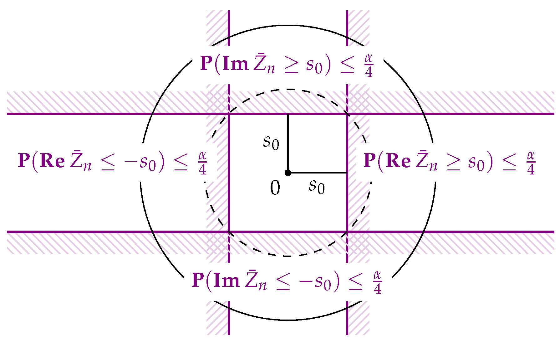
We will first consider the case of non-uniqueness of the circular mean, i.e., , or equivalently . Then, the critical value is well-defined for any and we get , and also, by considering , that . Analogously, . We conclude that
Rejecting the hypothesis , i.e., , if thus leads to a test whose probability of false rejection is at most α (see Figure 1). Of course, one may work with and as criterions for rejection; however, we prefer working with since it is independent of the chosen
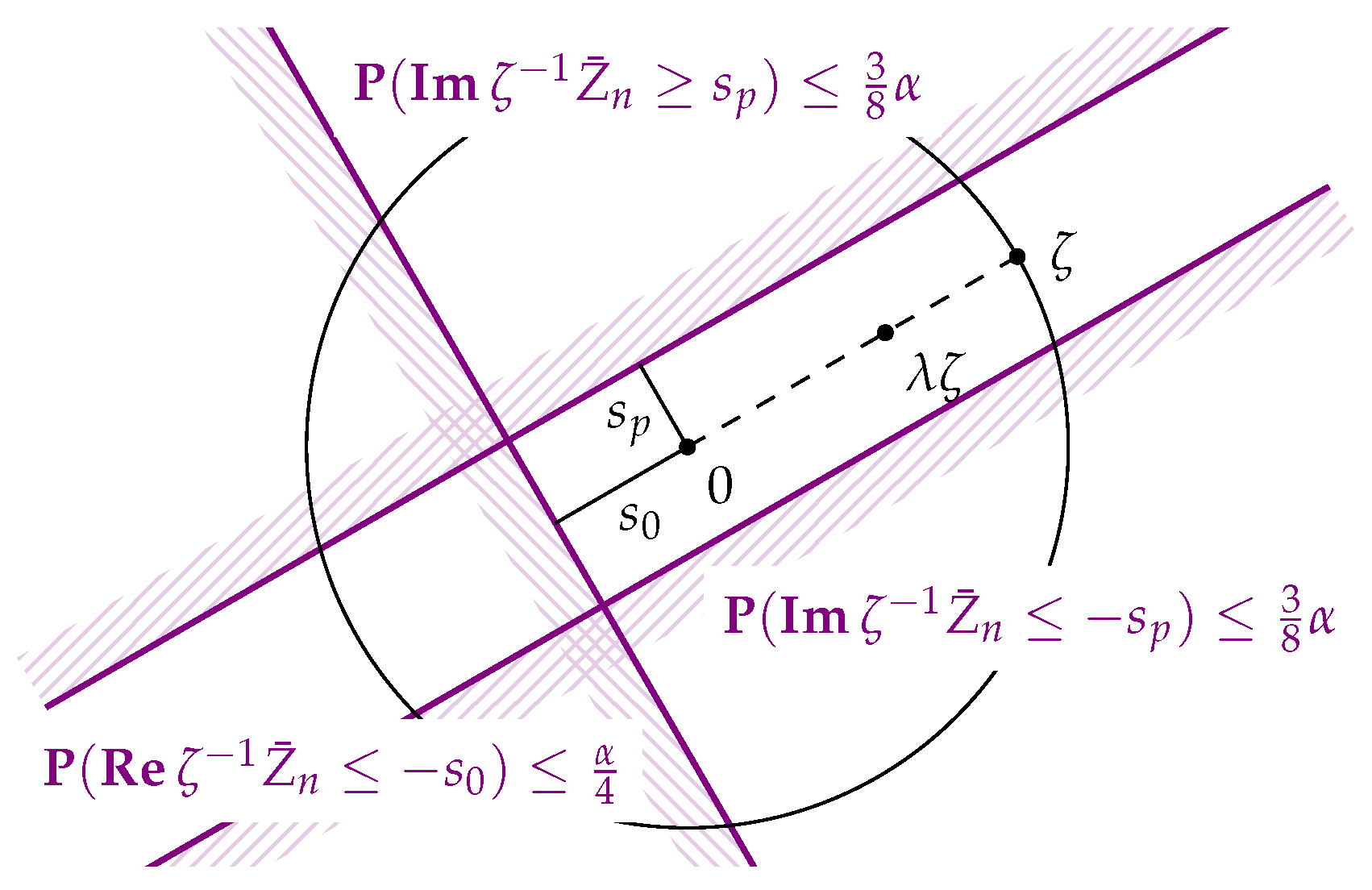
In the case of uniqueness of the circular mean, i.e., for the hypothesis , we use the monotonicity of in ν and obtain
as well. For the direction perpendicular to the direction of ζ (see Figure 2), however, we may now work with , so for —which is well-defined whenever is since —we obtain
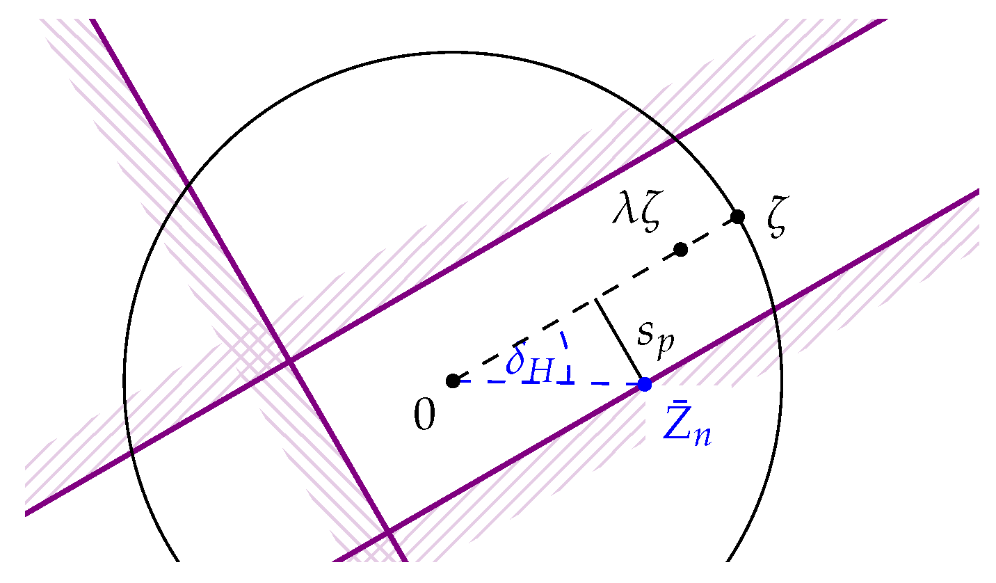
Rejecting if or , then, will happen with probability at most under the hypothesis . In case that we already rejected the hypothesis , i.e., if , ζ will not be rejected if and only if and which is then equivalent to (see Figure 3).
Define as all ζ which we could not reject, i.e.,
Then, we obtain the following result:
Proposition 1.
Let be random variables taking values on the unit circle , and let be defined as in Equation (8).
- (i)
- is a -confidence set for the circular population mean set. In particular, if , i.e., the circular population mean set equals , then with probability at most so indeed with probability at least
- (ii)
- and are of order .
- (iii)
- If then in probability and the probability of obtaining the trivial confidence set, i.e., , goes to 0 exponentially fast.
Proof.
(i) holds by construction.
For (ii), recall Equation (7), from which we obtain the estimates resp. , implying that and are of order the same holds stochastically for since a.s. Regarding the second statement of (iii), if μ is unique, consider ; then, and is eventually less than and also eventually. Hence, the probability of obtaining the trivial confidence set is eventually bounded by , and thus will go to zero exponentially fast as n tends to infinity. ☐
3. Estimating the Variance
From the central limit theorem for in case of unique μ, cf. Equation (4), we see that the aymptotic variance of gets small if is close to 1 (then is close to the boundary of the unit disc, which is possible only if the distribution is very concentrated) or if the variance in the direction perpendicular to μ is small (if the distribution were concentrated on , this variance would be zero and would equal μ with large probability). While ( being the denominator of its sine) takes the former into account, the latter has not been exploited yet. To do so, we need to estimate .
Consider that is under the hypothesis that the corresponding ζ is the unique circular population mean has expectation . Now, is the mean of n independent random variables taking values in and having expectation . By another application of Equation (6), we obtain for , the latter existing if . Since increases with , there is a minimal for which holds and becomes an equality; we denote it by . Inserting into Equation (6), it by construction fulfills
It is easy to see that the right-hand side depends continuously on and is strictly decreasing in (see Appendix A), thereby traversing the interval so that one can again solve the equation numerically. We then may, with an error probability of at most , use as an upper bound for . Note that exists if The latter is fulfilled for any since Equation (9) is equivalent to
For , let be the trivial bound.
With such an upper bound on its variance, we now can get a better estimate for . Indeed, one may use another inequality by Hoeffding [11] (Theorem 3): the mean of a sequence of independent random variables taking values in , each having zero expectation as well as variance fulfills
for any Again, an elementary calculation (analogous to Lemma A1) shows that the right-hand side of Equation (10) is strictly decreasing in w, continuously ranging between 1 and as w varies in , so that there exists a unique for which the right-hand side equals γ, provided . Moreover, the right-hand side increases with (as expected), so that is increasing in , too (cf. Appendix A).
Therefore, under the hypothesis that the corresponding ζ is the unique circular population mean, . Now, since , setting we get . Note that increases with , so in case exists, implies , i.e., the existence of .
Following the construction for from Section 2, we can again obtain a confidence set for μ with coverage probability at least as shown in our previous article [13]. In practice however, this confidence set is hard to calculate since has to be calculated for every Though these confidence sets can be approximated by using a grid as in [13], we suggest using a simultaneous upper bound for the variance of .
We obtain a (conservative) connected, symmetric confidence set by testing with as a common upper bound for the variance perpendicular to any . Note that can be obtained as the solution of Equation (9) with
Furthermore, we can shorten by iteratively redefining and recalculating (see Algorithm 1). The resulting opening angle will be denoted by
| Algorithm 1: Algorithm for computation of . |
 |
Proposition 2.
Let be random variables taking values on the unit circle and let
- (i)
- The set resulting from Algorithm 1 is a -confidence set for the circular population mean set. In particular, if , i.e., the circular population mean set equals , then with probability at most so indeed with probability of at least
- (ii)
- is of order .
- (iii)
- If i.e., if the circular population mean is unique, then in probability, and the probability of obtaining a trivial confidence set, i.e., , goes to 0 exponentially fast.
- (iv)
- If , thenwith denoting the -quantile of the standard normal distribution
Proof.
Again, (i) follows by construction, while (iii) is shown as in Proposition 1.
For (ii), note that since the bound in Equation (10) for agrees with the bound in Equation (6) for and thus and are at least of the order
For (iv), we will use the estimate in Equation (11). Recall that ; therefore, for large n and hence small a.s.
thus Additionally, for x close to 0 which gives a.s.
4. Simulation and Application to Real Data
We will compare the asymptotic confidence set , the confidence set constructed directly using Hoeffding’s inequality in Section 2, and the confidence set resulting from Algorithm 1 by reporting their corresponding opening angles , , and in degrees () as well as their coverage frequencies in simulations.
All computations have been performed using our own code based on the software package R (version 2.15.3) [14] .
4.1. Simulation 1: Two Points of Equal Mass at
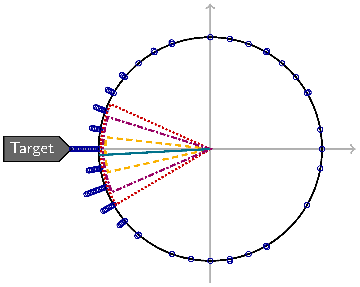
First, we consider a rather favourable situation: independent draws from the distribution with . Then, we have , implying that the data are highly concentrated, is unique, and the variance of Z in the direction of μ is 0; there is only variation perpendicular to μ, i.e., in the direction of the imaginary axis (see Figure 4).
Table 1 shows the results based on 10,000 repetitions for a nominal coverage probability of : the average is about times larger than , which is about twice as large as . As expected, the asymptotics are rather precise in this situation: did cover the true mean in about of the cases, which implies that the other confidence sets are quite conservative; indeed and covered the true mean in all repetitions. One may also note that the angles varied only a little between repetitions.
4.2. Simulation 2: Three Points Placed Asymmetrically
Secondly, we consider a situation which has been designed to show that even a considerably large sample size () does not guarantee approximate coverage for the asymptotic confidence set : the distribution of Z is concentrated on three points, , with weights chosen such that (implying a small variance and ), and , while . In numbers, , , and (in ) while , and (see Figure 5).
The results based on 10,000 repetitions are shown in Table 2 where a nominal coverage probability of was prescribed. Clearly, with its coverage probability of less than performs quite poorly while the others are conservative; still appears small enough to be useful in practice, though.
4.3. Real Data: Movements of Ants
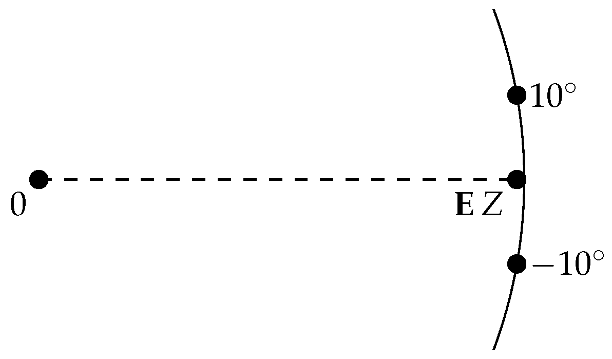
Fisher [3] (Example 4.4) describes a data set of the directions 100 ants took in response to an illuminated target placed at for which it may be of interest to know whether the ants indeed (on average) move towards that target (see [15] for the original publication). The data set is available as Ants_radians within the R package CircNNTSR [16].
The circular sample mean for this data set is about ; for a nominal coverage probability of , one gets , , and so that all confidence sets contain (see Figure 6). The data set’s concentration is not very high, however, so the circular population mean could—according to —also be or .
5. Discussion
We have derived two confidence sets, and , for the set of circular sample means. Both guarantee coverage for any finite sample size without making any assumptions on the distribution of the data (besides that they are independent and identically distributed) at the cost of potentially being quite conservative; they are non-asymptotic and universal in this sense. Judging from the simulations and the real data set, —which estimates the variance perpendicular to the mean direction—appears to be preferable over (as expected) and small enough to be useful in practice.
While the asymptotic confidence set’s opening angle is less than half (asymptotically about for ) of the one for in our simulations and application, it has the drawback that even for a sample size of , it may fail to give a coverage probability close to the nominal one; in addition, one has to assume that the circular population mean is unique. Of course, one could also devise an asymptotically justified test for the latter but this would entail a correction for multiple testing (for example working with each time), which would also render the asymptotic confidence set conservative.
Further improvements would require sharper “universal” mass concentration inequalities taking the first or the first two moments into account; however, this is beyond the scope of this article.
Acknowledgments
T. Hotz wishes to thank Stephan Huckemann from the Georgia Augusta University of Göttingen for fruitful discussions concerning the first construction of confidence regions described in Section 2. We acknowledge support for the Article Processing Charge by the German Research Foundation and the Open Access Publication Fund of the Technische Universität Ilmenau. F. Kelma acknowledges support by the Klaus Tschira Stiftung, gemeinnützige Gesellschaft, Projekt 03.126.2016.
Author Contributions
All authors contributed to the theoretical and numerical results as well as to the writing of the article. All authors have read and approved the final manuscript.
Conflicts of Interest
The authors declare no conflict of interest.
Appendix A. Proofs of Monotonicity
Lemma A1.
is strictly decreasing in
Proof.
We show the equivalent statement that is strictly decreasing in t:
Hence, and thus are strictly decreasing in ☐
Lemma A2.
Let be the solution to the equation Then, is strictly increasing in
Proof.
t is the solution of the equation
The derivatives of the left-hand side of Equation (A1) w.r.t. ν and t exist and are continuous. Furthermore, the derivative w.r.t. t does not vanish for any , cf. the proof of Lemma A1, whence the derivative exists by the implicit function theorem. When differentiating Equation (A1) with respect to one obtains
or equivalently
whence finishes the proof. ☐
Lemma A3.
The function
is strictly decreasing in
Proof.
We show the equivalent statement that is strictly decreasing in
☐
Lemma A4.
Let be the solution of the equation
Then, w is increasing in .
Proof.
w is the solution of the equation
The derivatives of the left-hand side of Equation (A2) w.r.t. and w exist and are continuous. Furthermore, the derivative w.r.t. w does not vanish for any : this derivative is
vanishing if and only if , i.e., if and only if which does not happen for Now, the derivative exists by the implicit function theorem. When differentiating Equation (A2) with respect to one obtains
or equivalently
Hence, if and only if , which holds since finishing the proof. ☐
References
- Mardia, K.V. Directional Statistics; Academic Press: London, UK, 1972. [Google Scholar]
- Watson, G.S. Statistics on Spheres; Wiley: New York, NY, USA, 1983. [Google Scholar]
- Fisher, N.I. Statistical Analysis of Circular Data; Cambridge University Press: Cambridge, UK, 1993. [Google Scholar]
- Jammalamadaka, S.R.; SenGupta, A. Topics in Circular Statistics; Series on Multivariate Analysis; World Scientific: Singapore, 2001. [Google Scholar]
- Mardia, K.V.; Jupp, P.E. Directional Statistics; Wiley: New York, NY, USA, 2000. [Google Scholar]
- Fréchet, M. Les éléments aléatoires de nature quelconque dans un espace distancié. Annales de l’Institut Henri Poincaré 1948, 10, 215–310. (In French) [Google Scholar]
- Hotz, T. Extrinsic vs. Intrinsic Means on the Circle. In Proceedings of the 1st Conference on Geometric Science of Information, Paris, France, 28–30 October 2013; Lecture Notes in Computer Science, Volume 8085. Springer-Verlag: Heidelberg, Germany, 2013; pp. 433–440. [Google Scholar]
- Afsari, B. Riemannian Lp center of mass: Existence, uniqueness, and convexity. Proc. Am. Math. Soc. 2011, 139, 655–673. [Google Scholar] [CrossRef]
- Arnaudon, M.; Miclo, L. A stochastic algorithm finding p-means on the circle. Bernoulli 2016, 22, 2237–2300. [Google Scholar] [CrossRef]
- Leeb, H.; Pötscher, B.M. Model selection and inference: Facts and fiction. Econ. Theory 2005, 21, 21–59. [Google Scholar] [CrossRef]
- Hoeffding, W. Probability Inequalities for Sums of Bounded Random Variables. J. Am. Stat. Assoc. 1963, 58, 13–30. [Google Scholar] [CrossRef]
- Boucheron, S.; Lugosi, G.; Massart, P. Concentration Inequalities : A Nonasymptotic Theory of Independence; Oxford University Press: Oxford, UK, 2013. [Google Scholar]
- Hotz, T.; Kelma, F.; Wieditz, J. Universal, Non-asymptotic Confidence Sets for Circular Means. In Proceedings of the 2nd International Conference on Geometric Science of Information, Palaiseau, France, 28–30 October 2015; Nielsen, F., Barbaresco, F., Eds.; Lecture Notes in Computer Science, Volume 9389. Springer International Publishing: Cham, Switzerland, 2015; pp. 635–642. [Google Scholar]
- R Core Team. R: A Language and Environment for Statistical Computing, version 2.15.3; R Foundation for Statistical Computing: Vienna, Austria, 2013. [Google Scholar]
- Jander, R. Die optische Richtungsorientierung der Roten Waldameise (Formica Rufa L.). Zeitschrift für Vergleichende Physiologie 1957, 40, 162–238. (In German) [Google Scholar] [CrossRef]
- Fernandez-Duran, J.J.; Gregorio-Dominguez, M.M. CircNNTSR: An R Package for the Statistical Analysis of Circular Data Using Nonnegative Trigonometric Sums (NNTS) Models, version 2.1. 2013.
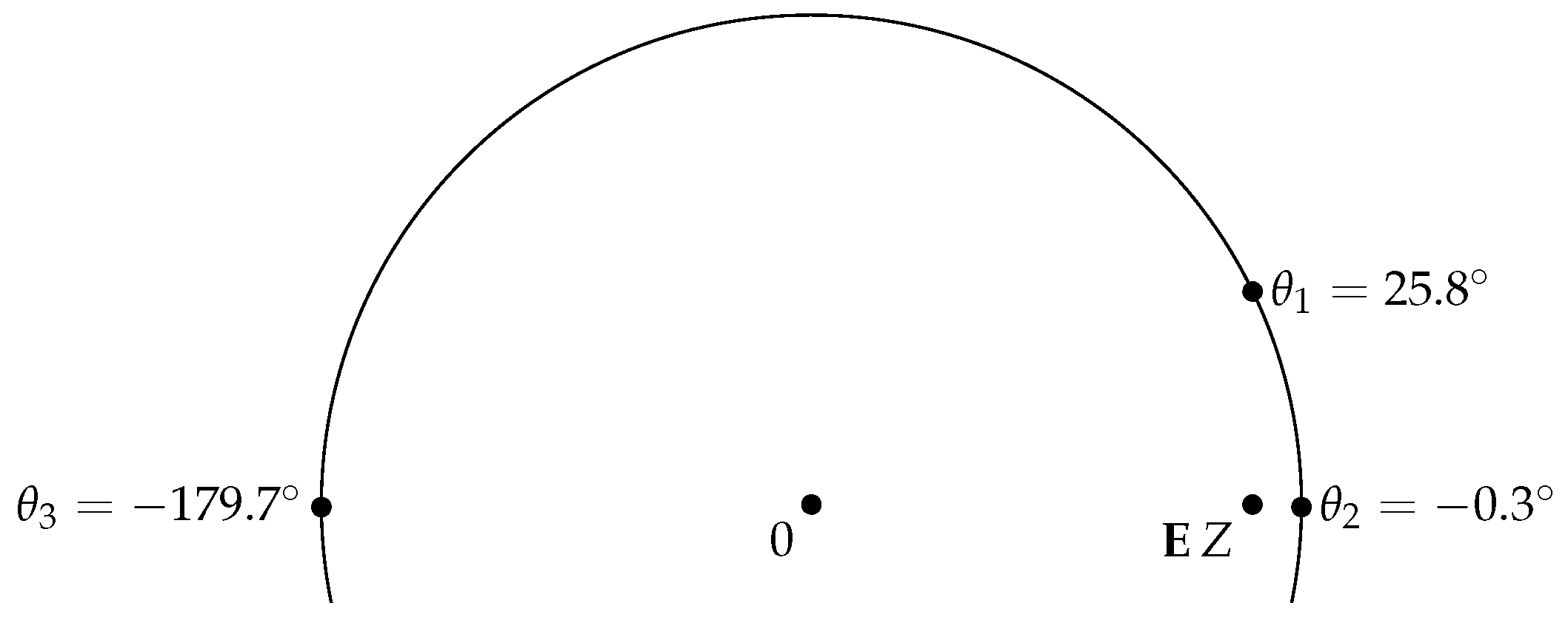
Figure 1.
The construction for the test of the hypothesis or equivalently

Figure 2.
The construction for the test of the hypothesis with .

Figure 3.
The critical regarding the rejection of ζ. bounds the angle between and any accepted

Figure 4.
Two points of equal mass at and their Euclidean mean.

Figure 5.
Three points placed asymmetrically with different masses and their Euclidean mean.

Figure 6.
Ant data ( ![Entropy 18 00375 i002]() ) placed at increasing radii to visually resolve ties; in addition, the circular mean direction (
) placed at increasing radii to visually resolve ties; in addition, the circular mean direction ( ![Entropy 18 00375 i003]() ) as well as confidence sets (
) as well as confidence sets ( ![Entropy 18 00375 i004]() ), (
), ( ![Entropy 18 00375 i005]() ), and (
), and ( ![Entropy 18 00375 i006]() ) are shown.
) are shown.
 ) placed at increasing radii to visually resolve ties; in addition, the circular mean direction (
  ) as well as confidence sets (
  ), (
), (  ), and (
  ) are shown.
Figure 6.
Ant data ( ![Entropy 18 00375 i002]() ) placed at increasing radii to visually resolve ties; in addition, the circular mean direction (
) placed at increasing radii to visually resolve ties; in addition, the circular mean direction ( ![Entropy 18 00375 i003]() ) as well as confidence sets (
) as well as confidence sets ( ![Entropy 18 00375 i004]() ), (
), ( ![Entropy 18 00375 i005]() ), and (
), and ( ![Entropy 18 00375 i006]() ) are shown.
) are shown.
) placed at increasing radii to visually resolve ties; in addition, the circular mean direction ( ) as well as confidence sets ( ), ( ), and ( ) are shown.

Table 1.
Results for simulation 1 (two points of equal mass at ) based on 10,000 repetitions with observations each: average observed , , and (with corresponding standard deviation), as well as frequency (with corresponding standard error) with which was covered by , , and , respectively; the nominal coverage probability was .
| Confidence Set | Mean δ (±s.d.) | Coverage Frequency (±s.e.) |
|---|---|---|
| () | () | |
| () | () | |
| () | () |
Table 2.
Results for simulation 2 (three points placed asymmetrically) based on 10,000 repetitions with observations each: average observed , , and (with corresponding standard deviation), as well as frequency (with corresponding standard error) with which was covered by , , and , respectively; the nominal coverage probability was .
| Confidence Set | Mean δ (±s.d.) | Coverage Frequency (±s.e.) |
|---|---|---|
| () | () | |
| () | () | |
| () | () |
© 2016 by the authors; licensee MDPI, Basel, Switzerland. This article is an open access article distributed under the terms and conditions of the Creative Commons Attribution (CC-BY) license (http://creativecommons.org/licenses/by/4.0/).
Share and Cite
MDPI and ACS Style
Hotz, T.; Kelma, F.; Wieditz, J. Non-Asymptotic Confidence Sets for Circular Means. Entropy 2016, 18, 375. https://0-doi-org.brum.beds.ac.uk/10.3390/e18100375
AMA Style
Hotz T, Kelma F, Wieditz J. Non-Asymptotic Confidence Sets for Circular Means. Entropy. 2016; 18(10):375. https://0-doi-org.brum.beds.ac.uk/10.3390/e18100375
Chicago/Turabian StyleHotz, Thomas, Florian Kelma, and Johannes Wieditz. 2016. "Non-Asymptotic Confidence Sets for Circular Means" Entropy 18, no. 10: 375. https://0-doi-org.brum.beds.ac.uk/10.3390/e18100375
Note that from the first issue of 2016, this journal uses article numbers instead of page numbers. See further details here.