Accelerating the Computation of Entropy Measures by Exploiting Vectors with Dissimilarity

Abstract

In the diagnosis of neurological diseases and assessment of brain function, entropy measures for quantifying electroencephalogram (EEG) signals are attracting ever-increasing attention worldwide. However, some entropy measures, such as approximate entropy (ApEn), sample entropy (SpEn), multiscale entropy and so on, imply high computational costs because their computations are based on hundreds of data points. In this paper, we propose an effective and practical method to accelerate the computation of these entropy measures by exploiting vectors with dissimilarity (VDS). By means of the VDS decision, distance calculations of most dissimilar vectors can be avoided during computation. The experimental results show that, compared with the conventional method, the proposed VDS method enables a reduction of the average computation time of SpEn in random signals and EEG signals by 78.5% and 78.9%, respectively. The computation times are consistently reduced by about 80.1~82.8% for five kinds of EEG signals of different lengths. The experiments further demonstrate the use of the VDS method not only to accelerate the computation of SpEn in electromyography and electrocardiogram signals but also to accelerate the computations of time-shift multiscale entropy and ApEn in EEG signals. All results indicate that the VDS method is a powerful strategy for accelerating the computation of entropy measures and has promising application potential in the field of biomedical informatics.

1. Introduction

In recent years, increasing attention has been paid to entropy measures for quantifying electroencephalogram (EEG) signals in neurological disease diagnosis and brain function assessment [1,2,3], including for monitoring of the depth of anesthesia [4,5], automatic detection of epileptic seizures [6,7] and estimation of cognitive workload [8,9], etc. Although numerous entropy measures have been proposed, such as approximate entropy (ApEn) [10], distribution entropy [11], bubble entropy [12], short-term Rényi entropy [13,14,15] and so on, many of them, such as ApEn, sample entropy (SpEn) [16], fuzzy entropy [17] and multiscale entropy (MSE) [18,19], require hundreds of data points for computation and involve high time costs. According to their definitions, their computational methods are based on phase space reconstruction by making use of many data points [20] and as such, arbitrary two vectors in the reconstructed phase space are required for distance calculation to determine whether the paired vectors are similar, leading to a great computational load.

In some specific applications of these entropy measures, if the computation is not performed fast enough, it is not practical for online neurological disease diagnosis or brain-state monitoring, especially for high-speed sampled data. To date, some advanced methods have been developed to achieve fast computation of entropy measures. On one hand, some fast algorithms have been proposed to accelerate the computation of entropy measures. Pan et al. developed a sliding k-dimensional tree (SKD) algorithm to speed up computation of SpEn and ApEn [21]. Although it was effective in a large number of data (for example, N > 2000), the SKD algorithm was observed to be inferior to the brute force algorithm for small values of N. Because when the data length N was short, both building and operating the tree involved a lot of overheads. Pan et al. also developed an adaptive SKD algorithm to overcome the shortcoming. The time complexity for SKD was O(N^3/2) as m = 2 for the real-type data. Manis et al. proposed a bucket-assisted algorithm for computation of ApEn [22]. The algorithm made use of the buckets of consecutive numbering to examine similar vectors only and it resembled the bucket-sort algorithm. The size of the required buckets was dependent on the actual data and algorithm parameter. In particular, when the data had outliers, the size of buckets would exceed the size of actual data. Sugisaki et al. introduced a recursive algorithm to perform online computation of SpEn [23] but the computational efficiency decreased with the decreasing overlap length of rolling windows. When the overlap length was zero, there was no improvement in computation time. Consider N data points with the overlap length N/2, the new N/2 data points were taken in and the old N/2 data points were removed at the new time. To perform the computation of SpEn, the recursive algorithm firstly removed only the information generated from the old data points, then took in only the information generated from the new data points and keeping the information generated from the other data points, consequently the calculation costs could be significantly reduced. Hong Bo et al. proposed a fast, practical algorithm of ApEn [24], which utilized a symmetrical distance matrix D and a binary matrix S to optimize the computational process and the distances between any two data points were considered. On the other hand, some entropy measures of low computational complexity have been developed [12,25,26] such as permutation entropy [25,26], which has been widely used in EEG signal analysis because of its simplicity and extremely fast computation [27,28,29].

By reviewing the available literature, we noticed that for ApEn, SpEn and MSE, most of research works directly calculated the distances of arbitrary two vectors to determine whether the paired vectors were similar according to their definitions of these entropy measures [30,31], ignoring vectors with dissimilarity. In this paper, we proposed a new method to accelerate computation of these entropy measures by exploiting vectors with dissimilarity (VDS). By adopting the proposed VDS method, the distance calculations of most of vectors were avoided because they were dissimilar as predetermined by the VDS decision and consequently the computation time was greatly reduced.

The remainder of this paper is organized as follows. Section 2 briefly introduces four typical entropy measures and their computation methods in accordance with their calculation steps. In addition, a detailed description of the VDS method is provided with respect to acceleration of the computation of these entropy measures and the details of method implementation and the testing program are given. Section 3 shows the experimental results and data analysis and provides a discussion. Finally, Section 4 summarizes our main points.

2. Methods

2.1. Approximate Entropy (ApEn) and Sample Entropy (SpEn)

ApEn was proposed by Pincus [10] and is widely applied in time series of physiological signals. SpEn is a modification of ApEn, introduced by Richman [16] and shows better performance with respect to consistency and dependence on data length. These entropy measures can quantify the system complexity as closely related to entropy. The computational methods are based on phase space reconstruction. Two sets of vectors with embedded dimensions m and m + 1 are constructed with hundreds of original data points and arbitrary two vectors are required to calculate their distances in order to determine their similarity. The computation methods of ApEn and SpEn are described in detail in the steps below.

Consider a time series X containing N data points:

$$X=\{x_1,x_2,x_3,\cdots ,x_N\},$$

(1)

A set of vectors is reconstructed from the time series X, denoted as ${\mathit{X}}_i^{(m)}$, whose embedded dimensions are m.

$${\mathit{X}}_i^{(m)}=(x_i,x_{i+2},x_{i+3},\cdots ,x_{i+m-1}),1\le i\le N-m,$$

(2)

The distance between two vectors is defined as

$$d\left({{\mathit{X}}_i}^{(m)},{{\mathit{X}}_j}^{(m)}\right)=\max \{\left|x_{i+k}-x_{j+k}\right|\},0\le k\le m-1,$$

(3)

The two vectors ${\mathit{X}}_i^{(m)}$ and ${\mathit{X}}_j^{(m)}$ are considered to be similar if the distance $d\left({\mathit{X}}_i^{(m)},{\mathit{X}}_j^{(m)}\right)$ is within r, where r is the tolerance for accepting matches,

For a given value of r, the counting variable C(i,j,r) is set to 1 when vectors ${\mathit{X}}_i^{(m)}$ and ${\mathit{X}}_j^{(m)}$ are similar to each other; otherwise, its value is set to zero.

$$C\left(i,j,r\right)=\{\begin{array}{l}1,d({\mathit{X}}_i^{(m)},{\mathit{X}}_j^{(m)})\le r\\ 0,otherwise\end{array},$$

(4)

For a given vector ${\mathit{X}}_i^{(m)}$, the number of vectors ${\mathit{X}}_j^{(m)}$ similar to vector ${\mathit{X}}_i^{(m)}$ is counted as $C^m\left(i,r\right)$.

$$C^m\left(i,r\right)={\displaystyle \sum _{j=1}^{N-m}{C}^m\left(i,j,r\right)},$$

(5)

Then, the probability of vector ${\mathit{X}}_i^{(m)}$ similar to any other vectors can be expressed as

$${P_i}^m\left(r\right)=\frac{1}{N-m}{C}^m\left(i,r\right),$$

(6)

Subsequently, as for ApEn, the first step is to take the natural logarithm of each $P_i^m(r)$ and then average it over i

$${\Phi }^m\left(r\right)=\frac{1}{N-m}{\displaystyle \sum _{i=1}^{N-m}\ln \left(P_i^m\left(i\right)\right)},$$

(7)

The second step is to increase the embedded dimension to m + 1 and to repeat the above calculation steps from Equations (2)–(7) to obtain $P_i^{m+1}(r)$ and Φ^m+1(r). Finally, the ApEn is computed as

$$ApEn\left(m,r\right)={\Phi }^m\left(r\right)-{\Phi }^{m+1}\left(r\right),$$

(8)

As for SpEn, there is a slight difference from the ApEn. It firstly averages $P_i^m(r)$ over i and then takes its natural logarithm.

$${\Psi }^m\left(r\right)=\ln \left(\frac{1}{N-m}{\displaystyle \sum _i^{N-m}{P}_i^m\left(r\right)}\right),$$

(9)

After that, the embedded dimension to m + 1 is increased and the above calculation steps are repeated to obtain $P_i^{m+1}(r)$ and ψ^m+1(r). Finally, the SpEn is given by

$$SpEn\left(m,r\right)={\Psi }^m\left(r\right)-{\Psi }^{m+1}\left(r\right)=\ln \left(\frac{{\displaystyle \sum _{i=1}^{N-m}{P_i}^m\left(r\right)}}{{\displaystyle \sum _{i=1}^{N-m}{P_i}^{m+1}\left(r\right)}}\right),$$

(10)

The SpEn differs from the ApEn mainly in the two ways [20]: (1) SpEn can remove the bias of self-matching; (2) SpEn performs additional operation prior to logarithmic operation so as to avoid the occurrence of the ln(0) in the calculations. Therefore, SpEn can require shorter data than ApEn and ApEn strongly depends on the length of data [16]. What’s more, SpEn has better relative consistency than ApEn [16].

2.2. Multiscale Entropy (MSE) and Time-Shift Multiscale Entropy (TSME)

The multiscale entropy (MSE) was introduced by Costa et al. and was developed to compute the corresponding SpEn in time series X over different scale factors [18,19]. The computation of MSE consists of two steps. Firstly, for the time series X of length N, a new coarse-grained time series is constructed by averaging the non-overlapping data points from X at a scale factor τ. Then, the SpEn is computed to obtain an entropy value for the coarse-grained time series. In general, the coarse-grained time series is obtained from X according to the following equation:

$$y_i^{(\tau )}=\frac{1}{\tau }{\displaystyle \sum _{i=(j-1)\times \tau +1}^{j\times \tau }{x}_i},1\le j\le \frac{N}{\tau },$$

(11)

Many modified versions of MSE have been developed to describe the multiscale properties of time series [32], such as composite multiscale entropy [33] and time-shift multiscale entropy (TSME) [34]. TSME was proposed by Pham [34], modifying the MSE over time series X of length N, with multiple time shifts at a given time interval kmax. The TSME is computed in the following three steps. Firstly, for a given time interval kmax, the k time-shift series is constructed from time series X by means of the known Higuchi’s fractal dimension [34,35]. Then, either the SpEn or ApEn is computed for all time-shift series, denoted as $TSM{E}_k^{\beta }$, β = 1, 2, ..., k. Finally, the TSME for each k is defined as the mean value of all $TSM{E}_k^{\beta }$ where k = 1, 2, ..., kmax [34]. With increasing k, the SpEn-based $TSM{E}_k^{\beta }$ can remain fairly constant, while the ApEn-based $TSM{E}_k^{\beta }$ tends to slightly decrease. The trend in the ApEn-based $TSM{E}_k^{\beta }$ should be due to the bias of self-matching in the computation of ApEn. Thus, the use of SpEn is more theoretically sound for computing TSME.

$$TSM{E}_k=\frac{1}{k}{\displaystyle \sum _{\beta =1}^{k}TSM{E}_k^{\beta }},$$

(12)

2.3. Vectors with Dissimilarity (VDS) Method

In order to accelerate the computation processes above, three strategies can be taken into consideration as shown below. First, the computational steps of Φ^m(r), Φ^m+1(r), ψ^m(r) and ψ^m+1(r) can be performed in parallel. Second, the distance $d({\mathit{X}}_i^{\left(m\right)},{\mathit{X}}_j^{\left(m\right)})$ is identical to $d({\mathit{X}}_j^{\left(m\right)},{\mathit{X}}_i^{\left(m\right)})$ and there is no need to calculate both distances. Third, the most time-consuming step is the distance calculation of $d({\mathit{X}}_i^{\left(m\right)},{\mathit{X}}_j^{\left(m\right)})$ and how to optimize this step is of the utmost importance for the overall computational load of the entropy measure. To the best of our knowledge, most of the published works adopted the first and the second strategies to reduce the computation time. Therefore, we focus on the third strategy to accelerate computation of entropy measures by exploiting VDS, which is referred to as the VDS method.

From a statistical point of view, according to the definitions and computation steps of entropy measures mentioned above, arbitrary two vectors with distances greater than r are generally superior in numbers. Thus, the number of the vectors with dissimilarity has a more obvious advantage than the number of the vectors with similarity and it is an extremely important to exploit a technique to determine whether the paired vectors are dissimilar before their distance calculations. Once the paired vectors are deemed to be dissimilar, there is no need to further calculate their distances, which can greatly reduce the computational time.

For SpEn and ApEn, two vectors of dimensions m are considered to be similar if their distances are within r, i.e.,

$$\left|x_{i+k}-x_{j+k}\right|\le r,\forall k,0\le k\le m-1,$$

(13)

Therefore, arbitrary two vectors of dimensions m are considered to be dissimilar if their scale components satisfy

$$\left|x_{i+k}-x_{j+k}\right|>r,\exists k,0\le k\le m-1,$$

(14)

We put forward a decision method to decide if the two vectors are dissimilar. The decision quantity, Decis(i,j), is defined as follows:

$$Decis(i,j)=\left|{\displaystyle \sum _{k=0}^{m-1}{x}_{i+k}}-{\displaystyle \sum _{k=0}^{m-1}{x}_{j+k}}\right|,$$

(15)

When the Decis(i,j) is greater than m × r, the corresponding paired vectors ${\mathit{X}}_i^{(m)}$ and ${\mathit{X}}_j^{(m)}$ are deemed to be dissimilar and this is referred to as the VDS decision. It can be proven as follows:

Assume that the Decis(i,j) is greater than m × r, it can be given by the formula:

$$\left|{\displaystyle \sum _{k=0}^{m-1}{x}_{i+k}-{\displaystyle \sum _{k=0}^{m-1}{x}_{j+k}}}\right|>m\times r,$$

(16)

$$\left|{\displaystyle \sum _{k=0}^{m-1}{x}_{i+k}-{\displaystyle \sum _{k=0}^{m-1}{x}_{j+k}}}\right|>m\times r\iff \left|{\displaystyle \sum _{k=0}^{m-1}(x_{i+k}-x_{j+k})}\right|>m\times r,$$

(17)

Because of |a| + |b| ≥ |a + b|, we can derive the following equation

$${\displaystyle \sum _{k=0}^{m-1}\left|(x_{i+k}-x_{j+k})\right|}>\left|{\displaystyle \sum _{k=0}^{m-1}(x_{i+k}-x_{j+k})}\right|,$$

(18)

From Equations (16) and (18), we can obtain

$${\displaystyle \sum _{k=0}^{m-1}\left|(x_{i+k}-x_{j+k})\right|}>m\times r,$$

(19)

In Equation (19), the sum of m absolute values, $\left|x_{i+k}-x_{j+k}\right|$ where k is 0, 1, ..., m − 1, is larger than m × r. For the m absolute values, assuming all absolute values of $\left|x_{i+k}-x_{j+k}\right|$ where k is 0, 1, ..., m − 1, are within r, then it can be deduced that

$$\max \{\left|(x_{i+k}-x_{j+k})\right|\}\le r,0\le k\le m-1\Rightarrow {\displaystyle \sum _{k=0}^{m-1}\left|(x_{i+k}-x_{j+k})\right|}\le m\times r,$$

(20)

By using reduction to absurdity, based on Equation (19), we can only deduce that

$$\max \{\left|(x_{i+k}-x_{j+k})\right|\}>r,0\le k\le m-1,$$

(21)

The maximum value of all absolute values is greater than r. Therefore, the paired vectors ${\mathit{X}}_i^{(m)}$ and ${\mathit{X}}_j^{(m)}$ are dissimilar.

By exploiting the VDS decision, some vectors can be predetermined to be dissimilar in the computation process and their distances are not necessary for further calculation for entropy measures. Furthermore, the vectors with dissimilarity are in fact superior in number, which also can be confirmed through experimental results in Section 3. Therefore, most of the time-consuming steps with regard to distance calculations between these paired vectors can be optimized during computation of entropy measures.

2.4. Implementation and Testing Method

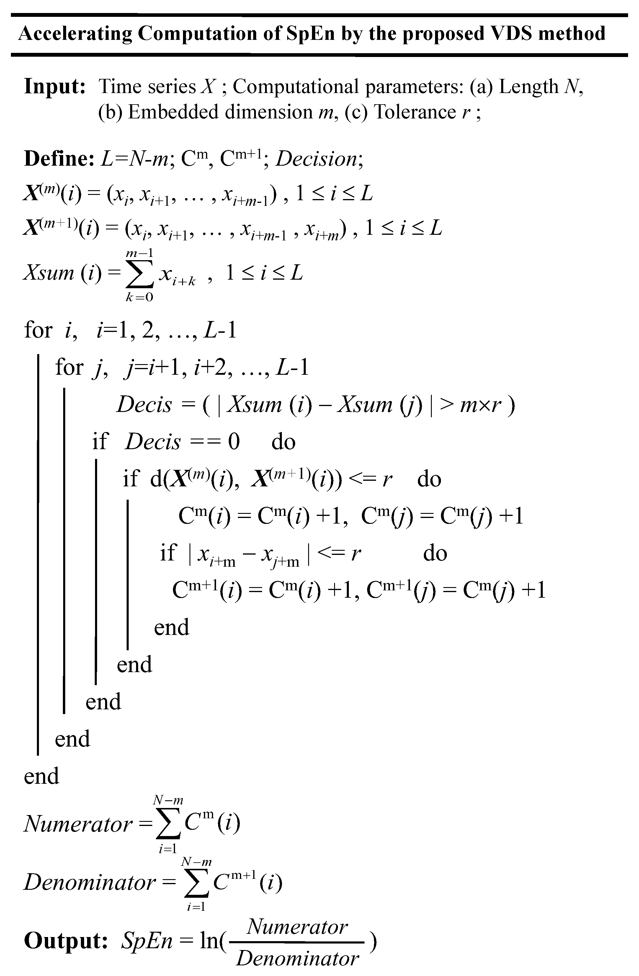
In order to test the performance of the proposed VDS method in accelerating the computation of entropy measures taking SpEn as an example, we implemented the VDS method for accelerating the computation of SpEn in Figure 1. The details of implementation of the proposed VDS method for accelerating computation of SpEn are explained as follows.

(1)

The input quantities are the time series X and computational parameters N, m, r.

(2)

Two sets of vectors ${\mathit{X}}^{(m)}$ and ${\mathit{X}}^{(m+1)}$ are reconstructed from the original time series X. Their embedded dimensions are m and m + 1, respectively and the sizes are both L = N − m.

(3)

All scalar components of each vector ${\mathit{X}}^{(m)}(i)$ are added to obtain the Xsum(i).

(4)

For arbitrary two vectors, if the absolute value of Xsum (i) − Xsum (j) is greater than m × r, the Decis for the paired vectors ${\mathit{X}}^{(m)}(i)$ and ${\mathit{X}}^{(m)}(j)$ is set to 1 and then there are no further steps to calculate their distance.

(5)

Otherwise, the Decis is set to 0 and for the paired vectors there are some calculation steps needed to further calculate their distance in order to determine whether they are similar. An array C^m is used for saving and updating the counting variable. If the distance of the paired vectors is within r, the C^m(i) and C^m(j) both increase by 1.

(6)

When the $d({\mathit{X}}^{(m)}(i),{\mathit{X}}^{(m)}(j))\le r$ holds, the paired vectors of embedded dimension m are deemed to be similar. Then we continue to check whether the distance of the paired vectors of embedded dimension m + 1 is within r. Another array C^m+1 is used for saving and updating the counting variable.

(7)

Finally, the SpEn is computed.

In order to better study the time efficiency of the VDS method, we also developed a conventional method to compute the SpEn as a contrast. For the conventional method, most of the calculation steps were the same as in the VDS method, only without the steps of the VDS decision.

Furthermore, for quantitative analysis of the VDS method to better understand the operation principle of accelerating computation, we developed a testing program to count the number of paired vectors for which Decis = 1 in Figure 1. The testing program added the some counting steps on the basis of the VDS method. We developed the testing program rather than directly using the VDS method to count, mainly because the counting steps would cause an increase in the running time of the VDS method, which was not conducive to evaluating the time efficiency correctly.

3. Results and Discussion

3.1. Experimental Data

We used two kinds of signals to evaluate time efficiency of computation of SpEn and TSME. One was random signal uniformly distributed in the interval (0, 1) and the other was the EEG signal. It is well known that most of physiological signals, for example EEG signals, have a characteristic of randomness in the time domain [36]. The EEG signals were obtained from the EEG motor movement/imagery dataset (EEGMMID) [37] found at http://www.physionet.org. The EEG signals were recorded using the BCI2000 system from 64 electrodes as per the international 10–10 system. The subjects performed different motor/imagery tasks while 64-channel EEG signals were recorded and sampled at 160 samples per second. We optionally selected some subjects’ EEG signals to use for computation of SpEn and TSME.

3.2. Accelerating Computations of Sample Entropy (SpEn) in Random Signals and White Noises

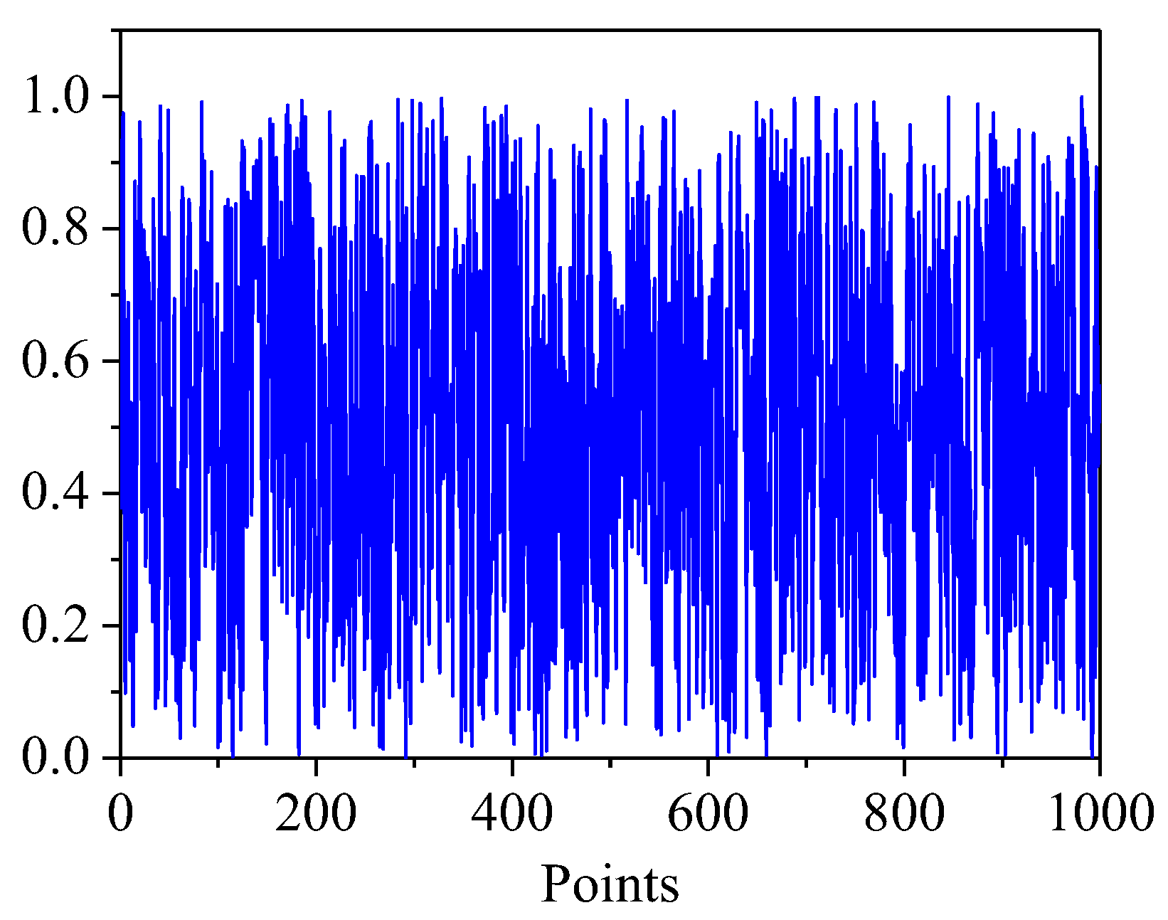
First of all, we used ten random signals to assess the VDS method in the accelerating computation of SpEn. Each random signal has 1000 data points uniformly distributed in the interval (0, 1), as shown in Figure 2.

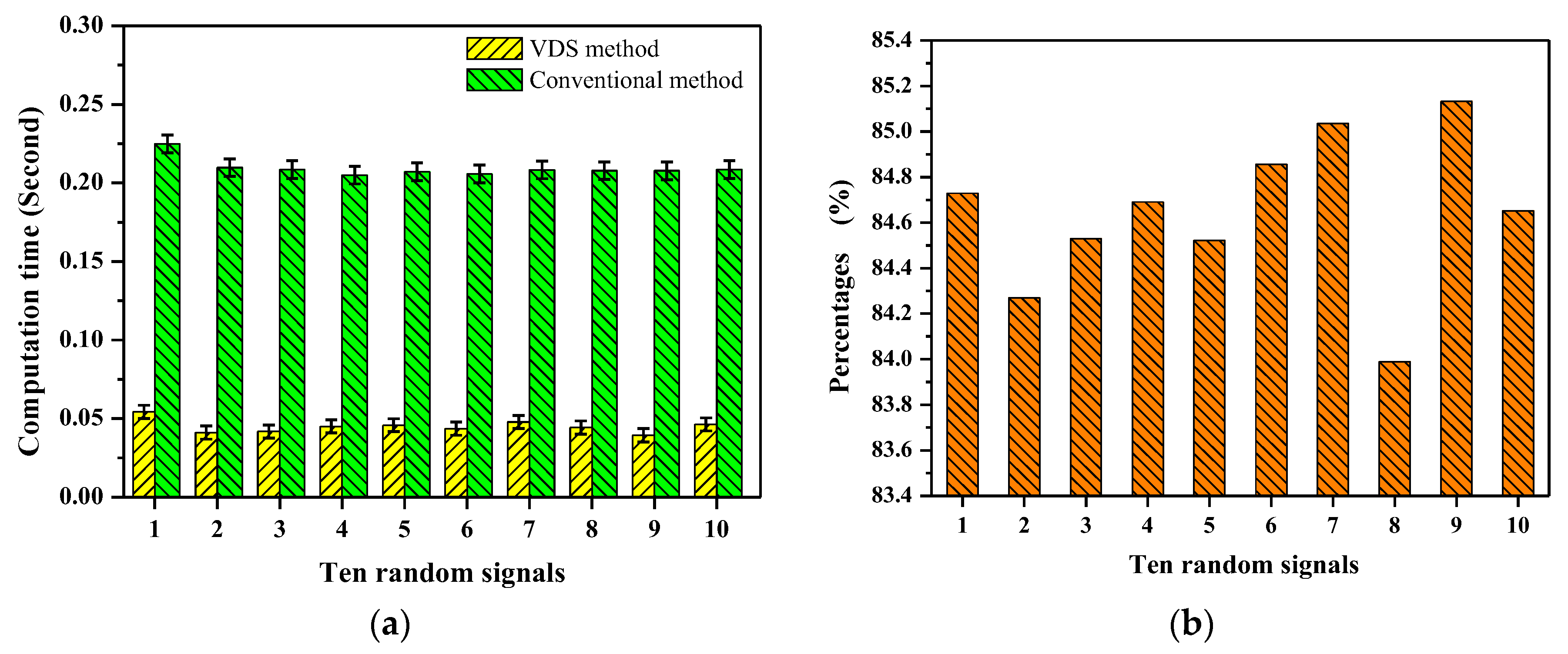
To evaluate time efficiency of computation, we adopted both the VDS method and the conventional method to compute SpEn in the ten random signals and measured the computation time. The computational parameters of SpEn are N = 1000, m = 2 and r = 0.2 × STD, where STD is the standard deviation of each random signal. The measurement values of SpEn by the adoption of the VDS and conventional method are identical. Figure 3a presents the computation time of SpEn in the ten random signals. It is clearly observed that the computation of SpEn is greatly accelerated by the adoption of the VDS method. The mean computation time is calculated by averaging the ten random signals. For the conventional method the mean computation time of SpEn is 0.209 s but for the VDS method it is only 0.045 s. Consequently, the computation time of SpEn is significantly (p < 0.005) reduced, by 78.5%. The standard deviations of the computation time for the VDS and conventional method are 0.0042 and 0.0056, respectively.

For quantitative analysis, it is necessary to study how many vectors are determined to be dissimilar by the VDS decision in the computation process. Utilizing the testing program, the SpEn in the ten random signals was computed once again and the number of the paired vectors which were dissimilar as determined by the VDS decision was counted. Then, the percentages of these paired vectors were calculated. Figure 3b shows that the percentages of the paired vectors which are dissimilar as determined by the VDS decision are 84.7%, 84.3%, 84.5%, 84.7%, 84.5%, 84.9%, 85.1%, 84.0%, 85.1% and 84.7% for the ten random signals during computation. The paired vectors which are dissimilar indicate that their distances are greater than r. This experimental result reveals the fact that arbitrary two vectors with dissimilarity are superior in numbers for the computation of entropy measures.

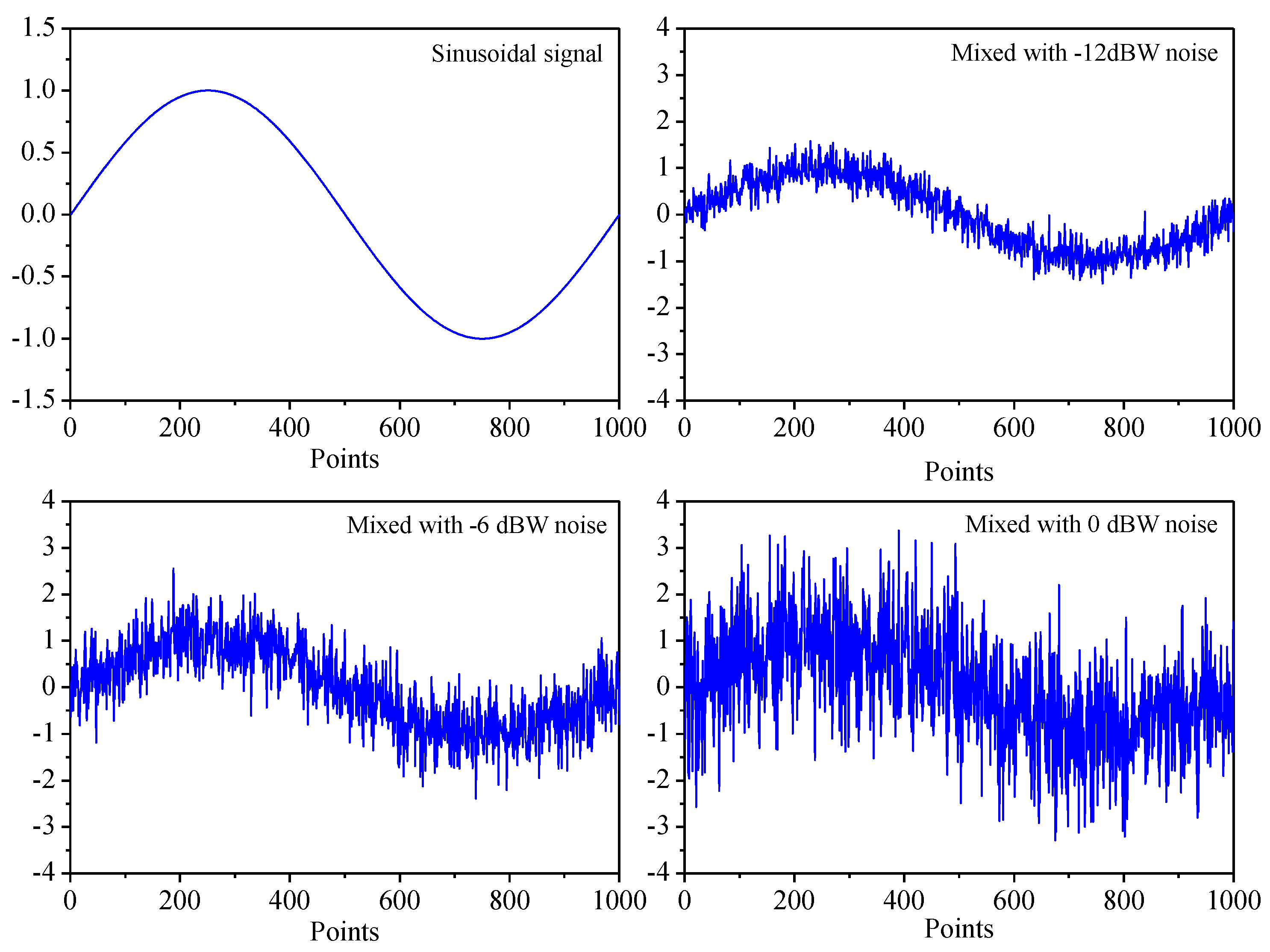
Furthermore, we analyzed several types of white noises of different power and mixed them with sinusoidal signal to evaluate the VDS method and compare against the conventional method. Six white noises’ powers, −12 dBW, −9 dBW, −6 dBW, −3 dBW, 0 dBW and 3 dBW, respectively, were investigated and mixed with sinusoidal signal. Figure 4 presents the sinusoidal signal and the mixed-signals with white noises of power −12 dBW, −6 dBW and 0 dBW, respectively.

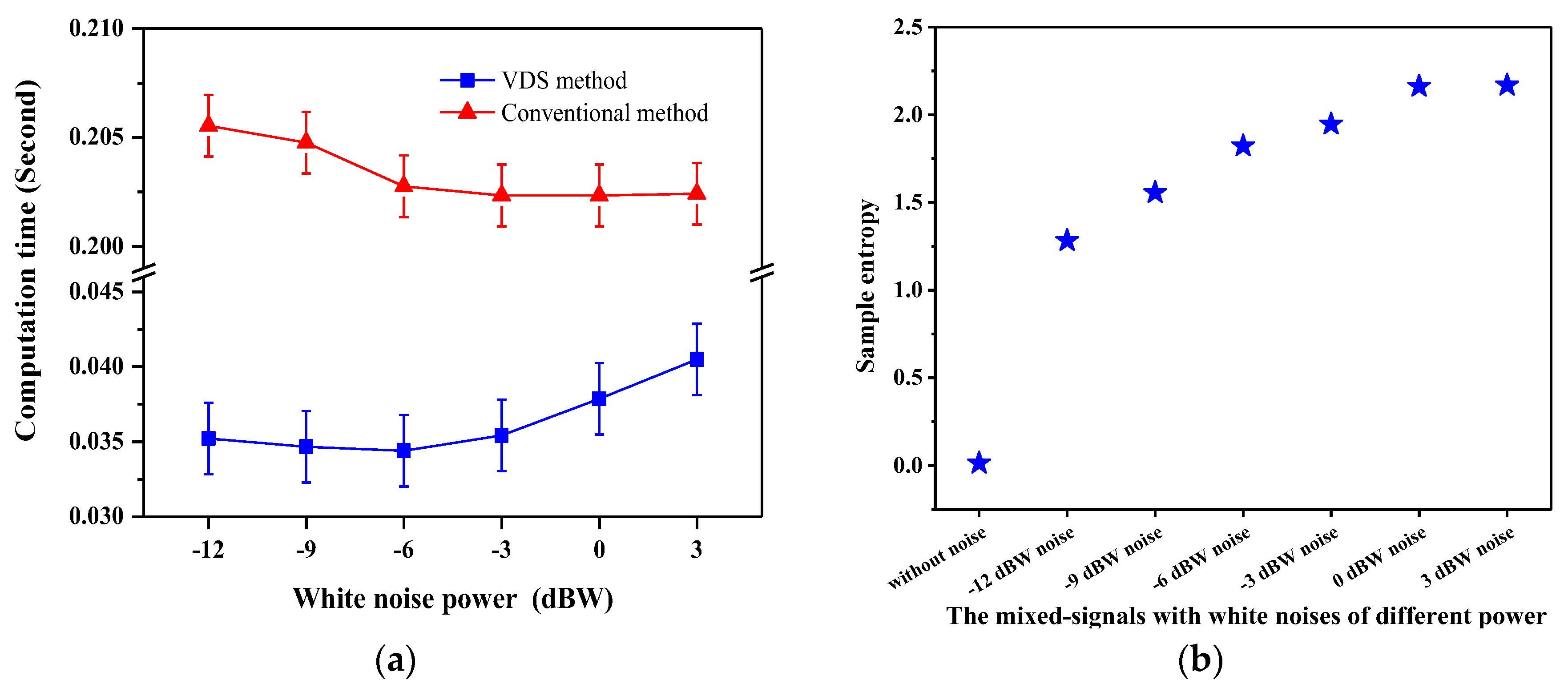
Figure 5a shows the computation times of SpEn in the six mixed-signals using the VDS and conventional method with the computational parameters N = 1000, m = 2 and r = 0.2 × STD, where STD is the standard deviation of each mixed-signal. It is clearly observed that the computation time of the VDS method is significantly (p < 0.005) lower than that of the conventional method. For the VDS method the changing trend of the computation time increases with the white noise’s power increase. Figure 5b shows the measurement values of SpEn in the sinusoidal signal and six mixed-signals. The measurement values of SpEn by the adoption of the VDS and conventional method are identical. The larger power of the white noise the mixed-signal is mixed with, the greater value of SpEn in the mixed-signal is and the value of SpEn in the mixed-signal would reach a certain limit with the increase of the white noise’s power.

3.3. Accelerating Computation of Sample Entropy (SpEn) in EEG Signals

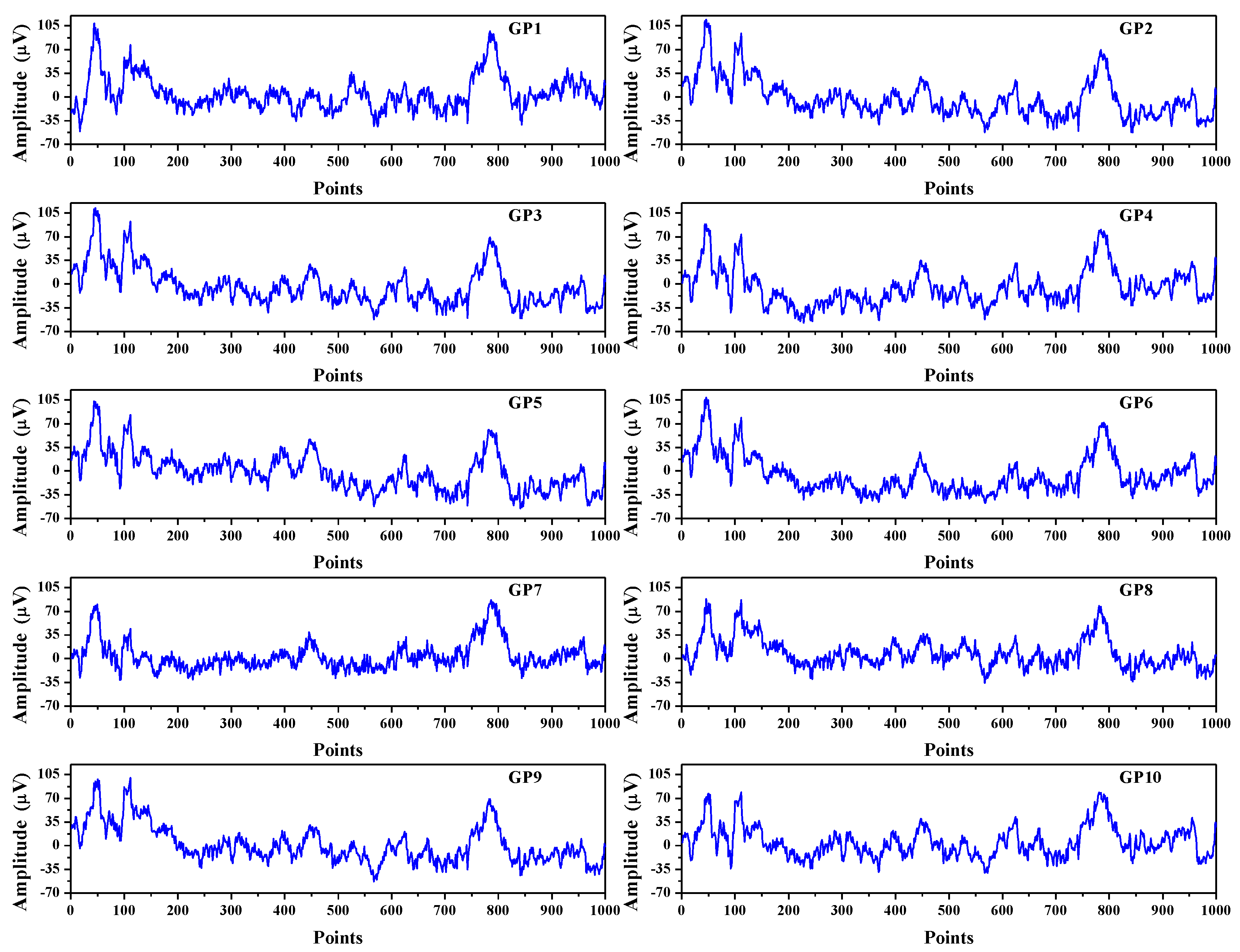
In order to demonstrate practical application of the VDS method in entropy measures, the computation of SpEn in EEG signals was investigated. The EEG signals were from the EEGMMID, which corresponded to the first set of experimental data of the subject labeled S011. Although the signals were of 64 channels in the records, the first ten channels of signals were used to compute SpEn. Figure 6 shows the ten channels’ EEG signals and the lengths of EEG signals are N = 1000. The vertical axis indicates the amplitude of EEG signals; the units are microvolts.

By adopting the VDS and conventional method, we computed the SpEn in the EEG signals and measured the computation time with the computational parameters N = 1000, m = 2, r = 0.2 × STD, where STD was the standard deviation of each EEG signal.

Table 1. The measurement of SpEn in the ten channels’ EEG signals. The computational parameters are N = 1000, m = 2, r = 0.2 × STD, where STD is the standard deviation of each EEG signal. The channel numbers from CH1 to CH10 correspond to the ten channels’ EEG signals.

Channel Number	SpEn	Channel Number	SpEn
CH1	0.9152	CH6	0.8501
CH2	0.8178	CH7	1.0800
CH3	0.8109	CH8	1.0609
CH4	0.8298	CH9	0.7931
CH5	0.8491	CH10	0.9785

gives the measurement results of SpEn in the ten channels’ EEG signals. The measurement values of SpEn by the adoption of the VDS and conventional method are identical.

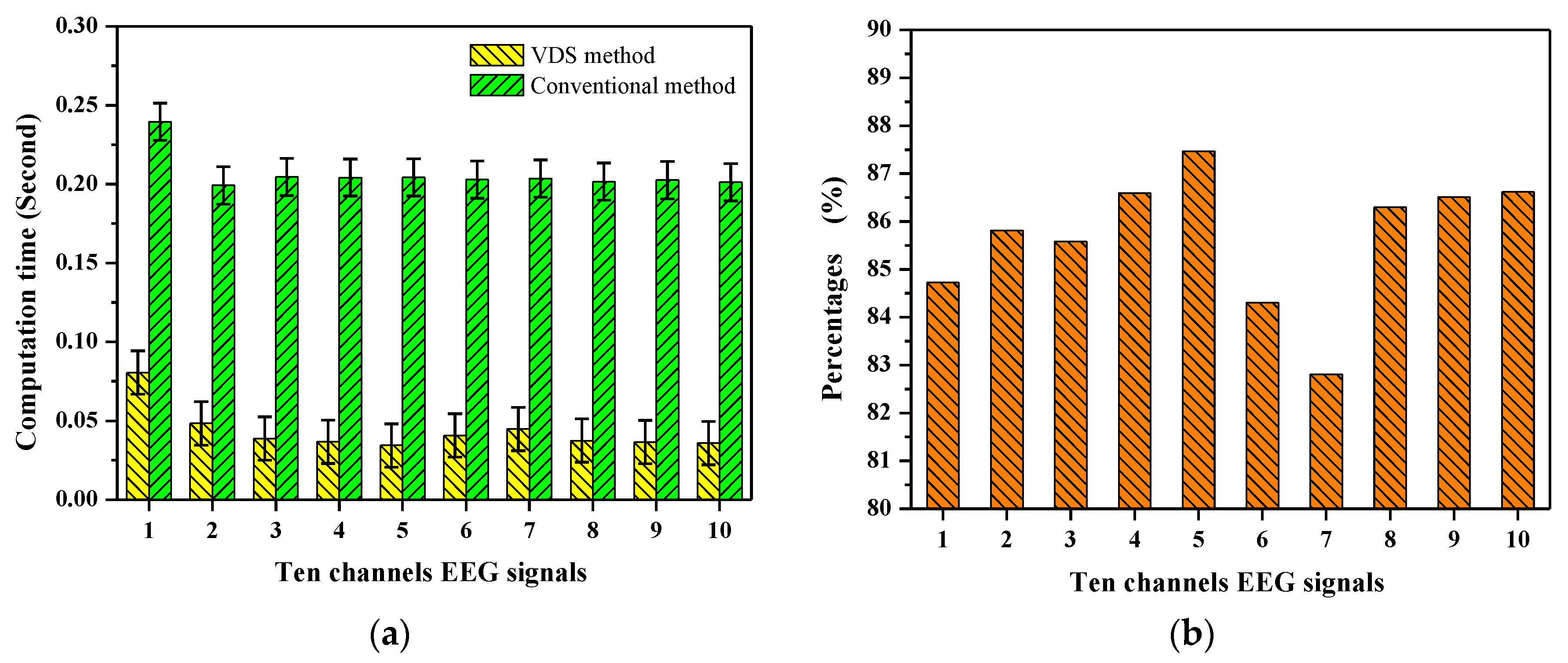
Figure 7a presents the computation time of SpEn in the ten channels’ EEG signals. The mean computation times are 0.0434 s and 0.2063 s for the VDS and conventional method, respectively. The standard deviation of the computation time for the VDS method is greater than that for the conventional method. These experimental results indicate that the mean computation time of SpEn is greatly (p < 0.005) reduced using the VDS method, by 78.96%.

To count the number of vectors which were determined to be dissimilar by the VDS decision during computation, the SpEn in the ten channels’ EEG signals was computed once again by the testing program. The percentages of vectors which are dissimilar as determined by the VDS decision in the computation process are calculated as shown in Figure 7b. The results are 84.7%, 85.8%, 85.6%, 86.6%, 87.5%, 84.3%, 82.8%, 86.3%, 86.5% and 86.6% for the ten channels’ EEG signals. The experimental results reveal that about 85.6% of arbitrary two vectors are deemed to be dissimilar for the ten channels’ EEG signals, as determined by the VDS decision. Their distances are avoided in calculations to determine whether or not they are similar during the computation of the SpEn.

We investigated the influence of parameter N and r on the time efficiency of computation. The computation of SpEn in the ten channels’ EEG signals with five kinds of lengths was performed by adopting the VDS method and the conventional method and involved measurement of the computation times. The five lengths selected were N = 500, N = 1000, N = 2000, N = 4000 and N = 8000 and the other computational parameters were m = 2 and r = 0.2 × STD, where STD was the standard deviation of each EEG signal. For each given length’s EEG signals, the mean computation time of SpEn was calculated by averaging the ten channels’ EEG signals, as shown in

Table 2. The mean computation time of SpEn in EEG signals with five kinds of lengths. The five lengths are: N = 500, N = 1000, N = 2000, N = 4000, N = 8000, respectively; the other computational parameters are m = 2 and r = 0.2 × STD, where STD is the standard deviation of each EEG signal.

Mean Time (s)	N = 500	N = 1000	N = 2000	N = 4000	N = 8000
VDS method	0.0102	0.0399	0.1420	0.5585	2.2037
Conventional method	0.0514	0.2023	0.8012	3.2410	12.843
Time-reduced rate (%)	80.1	80.3	82.3	82.8	82.8

. For the lengths of N = 500, N = 1000, N = 2000, N = 4000, N = 8000, the time-reduced rates of computation of SpEn using the VDS method were 80.1%, 80.3%, 82.3%, 82.8% and 82.8%, respectively, as compared with the conventional method.

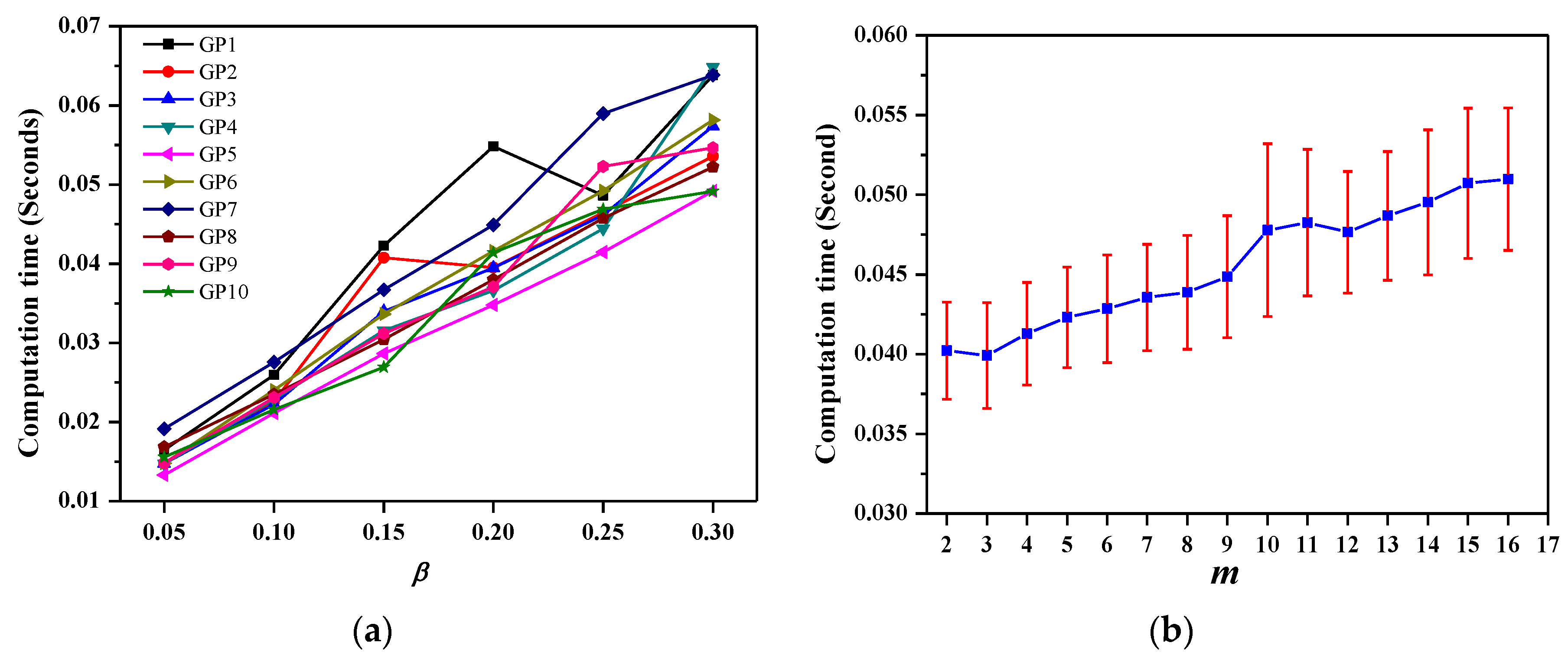
We investigated the computation time of SpEn in the ten channels’ EEG signals with different r parameters by the VDS method. The variable β was defined in the parameter r, r = β × STD. The value of β ranged from 0.05 to 0.3, with an increase by step length 0.05. The other computational parameters were N = 1000 and m = 2. We performed the computation of SpEn in ten channels’ EEG signals by adopting the VDS method and measured their computation times. Figure 8a shows the changes in computation times of SpEn over different r parameters. For each channel’s EEG signals, the computation time of SpEn increases to almost the same degree as the value of parameter r and the greater the value of parameter r is, the longer the computation time is.

We further checked the efficiency of the VDS method for different m parameters. The value of m ranged from 2 to 17 and the other computational parameters N = 1000 and r = 0.2 × STD. Figure 8b shows the computation time over different m parameters and the computation time is given as the means ± standard error. It is clearly observed that the mean computation time of SpEn increases with the increase of the value of parameter m.

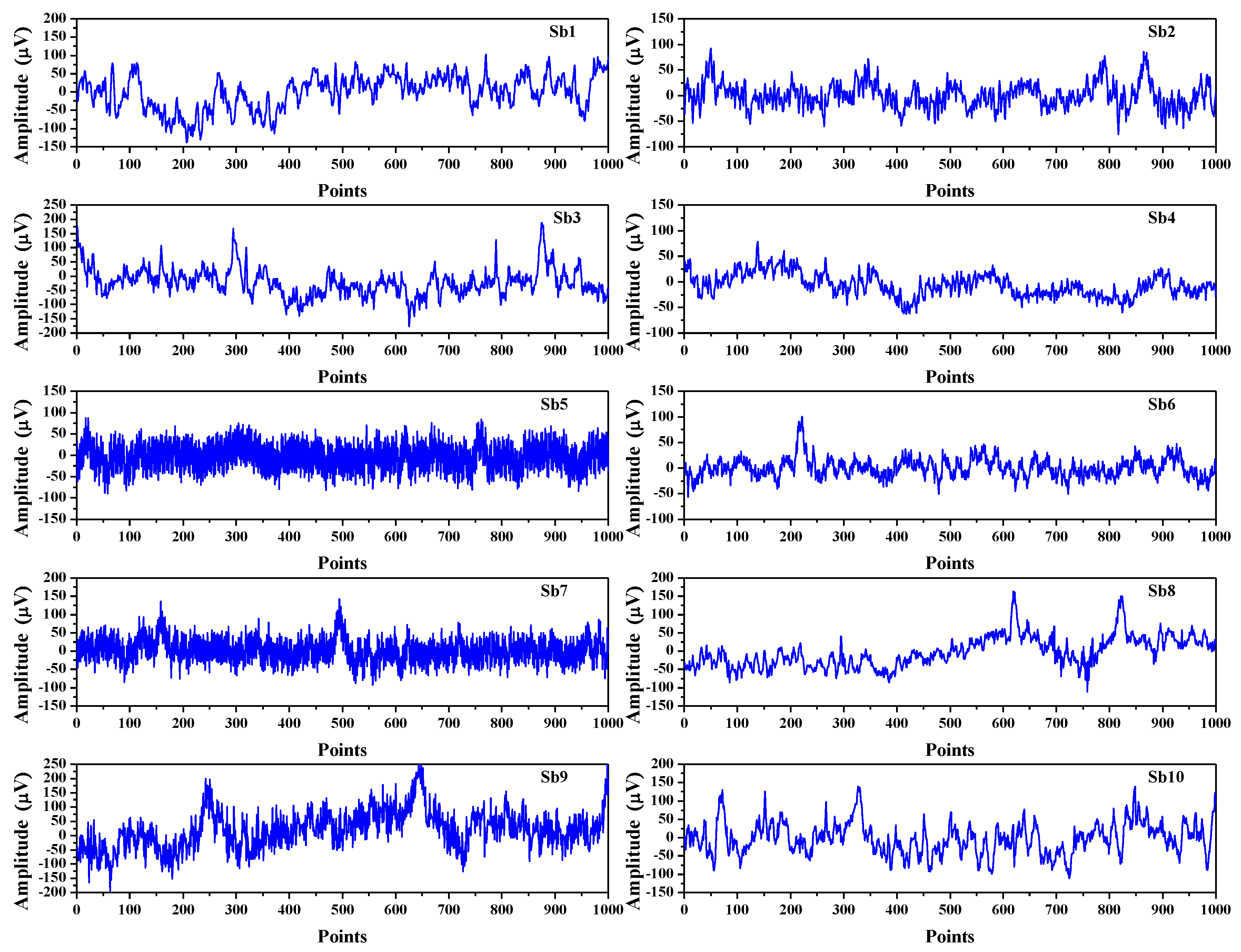
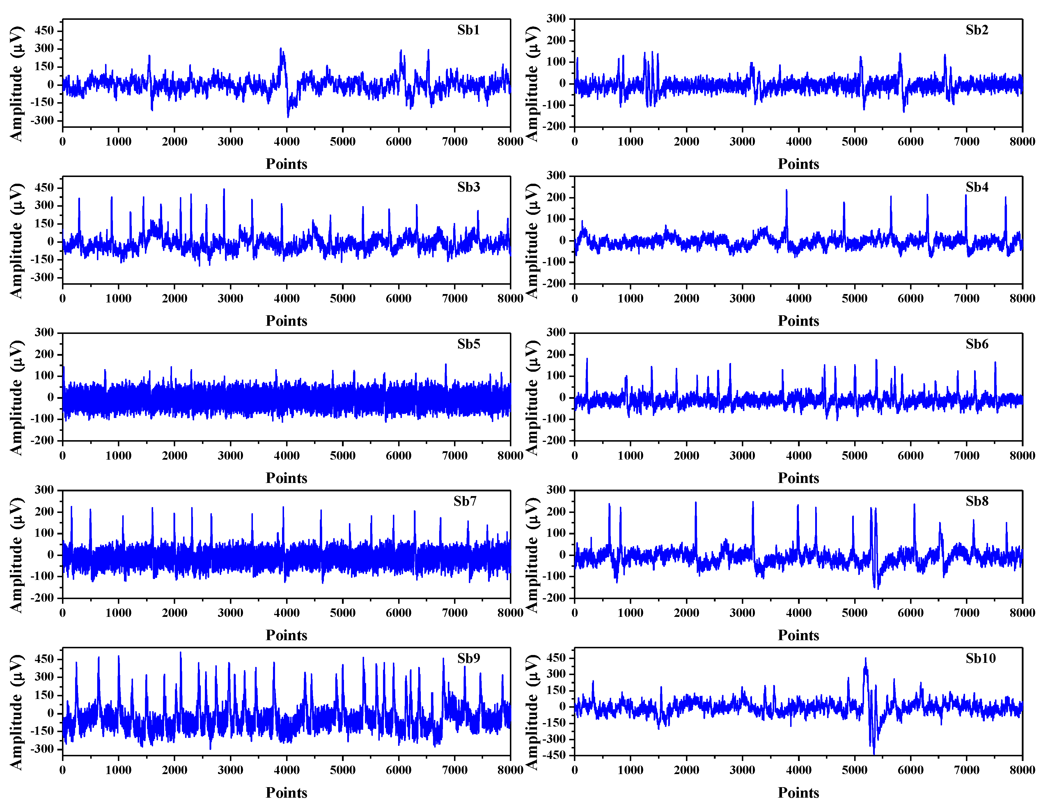
In order to evaluate the robustness of the VDS method, we carried out the computation of SpEn with the EEG signals of ten subjects. The ten subjects’ EEG signals were from the EEGMMID, which was the first set of experimental data of the subjects labeled from S001 to S010, corresponding to the electrode name Cz (numbering 11 in the records). The ten subjects’ EEG signals are shown in Figure 9.

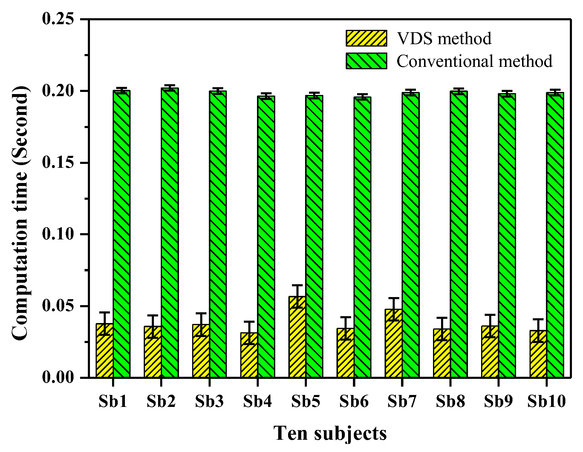
Figure 10 shows that the computation time of SpEn in the ten subjects’ EEG signals by the VDS and conventional method. For the conventional method, the mean computation time of SpEn in the ten subjects’ EEG signals is 0.199 s but for the VDS method the mean computation time of SpEn is 0.038 s, thus the computation time is significantly (p < 0.005) reduced by 80.9%. The standard deviation of the computation time for the VDS method is greater that for the conventional method. The measurement values of SpEns by adoption of the VDS and conventional method are identical and are 1.12, 1.52, 1.32, 1.40, 1.36, 1.80, 1.57, 0.97, 1.87 and 1.30, respectively. This experimental result indicates that the VDS method is sufficiently robust and effective for accelerating computation of SpEn in the EEG signals for different subjects.

3.4. Accelerating Computations of SpEn in Electromyography (EMG) and Electrocardiogram (ECG) Signals

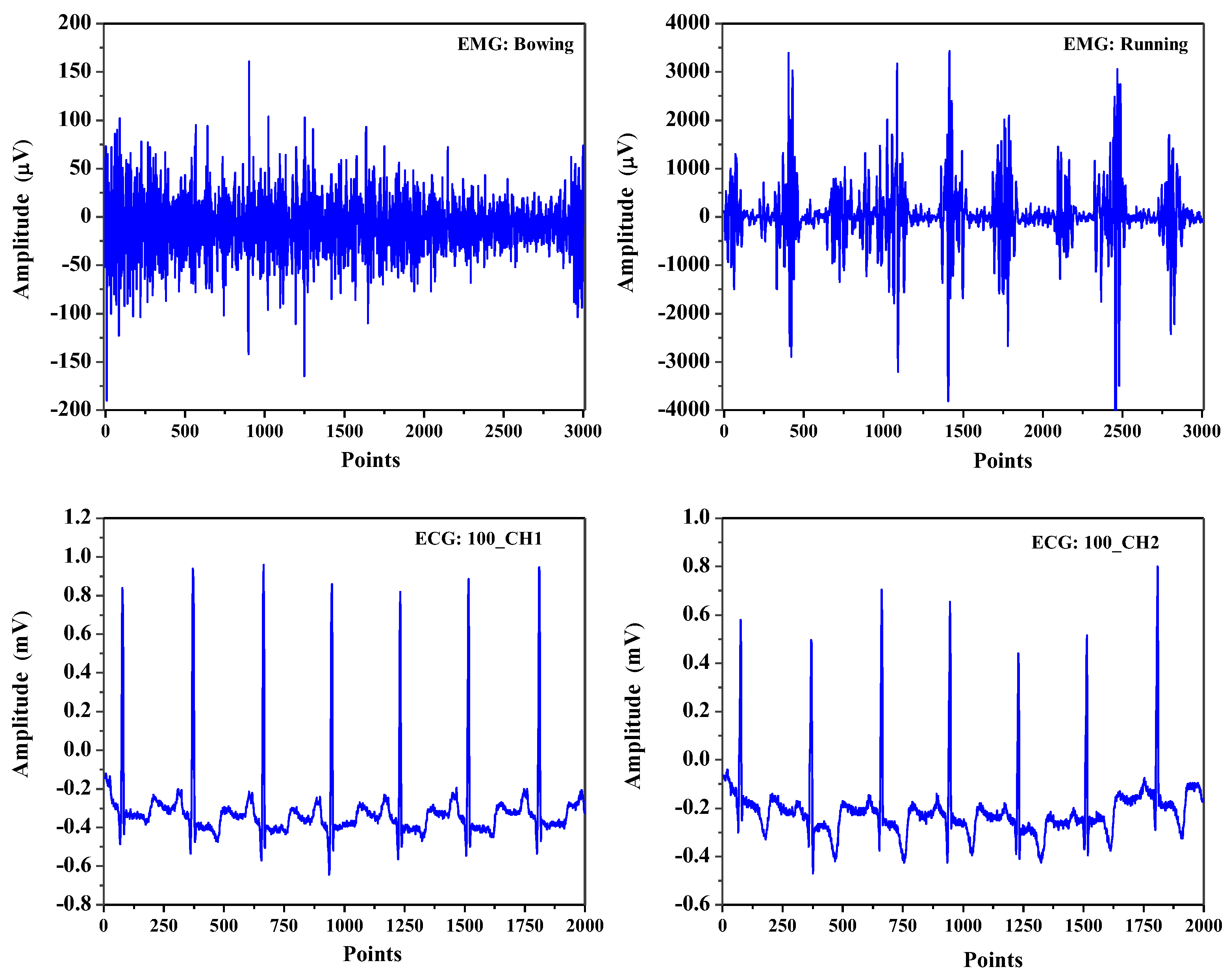
In order to demonstrate the robustness and data-dependent of the VDS method, we further analyzed the electromyography (EMG) and electrocardiogram (ECG) signals. The EMG signals were obtained from the Physical Action Data Set [38], which included 10 normal and 10 aggressive physical actions that measured the human activity from 4 subjects. In our study, the EMG signals were selected from the channel measured on the right bicep of the first subject and contained eight normal physical actions: (1) bowing; (2) handshaking; (3) hugging; (4) seating; (5) walking; (6) jumping; (7) standing; and (8) running. The ECG signals were obtained from the MIT-BIH Arrhythmia Database [37], where contained 48 half-hour excerpts of two-channel ambulatory ECG recordings and were digitized at 360 samples per second. In our study, the ECG signals used were the recording data numbering 100, 101, 112 and 217 in the records. Figure 11 shows the first 3000 samples of the EMG signals of two normal actions, bowing and running and the first 2000 samples of the ECG signals numbering 100 in the records.

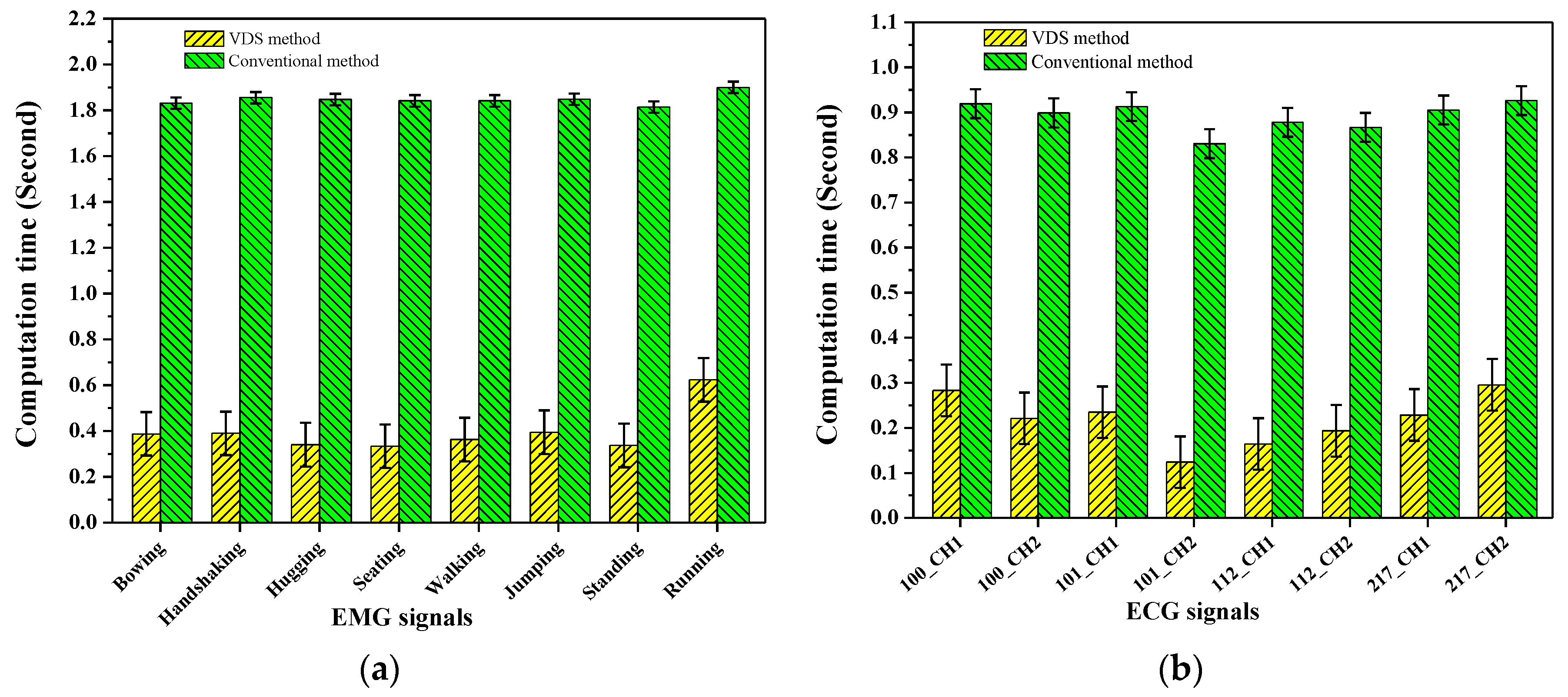
We computed the SpEn in the eight EMG signals using the VDS and conventional method with the computational parameters N = 3000, m = 2, r = 0.2 × STD, where STD was the standard deviation of each EMG signal. Figure 12a shows that the computation time of SpEn in the eight EMG signals. For the conventional method the mean computation time of SpEn is 1.848 s but for the VDS method the mean computation time of SpEn is 0.396 s. Therefore the computation time is significantly (p < 0.005) reduced using the VDS method. The standard deviation of the computation time for the VDS method is greater than that for the conventional method. The measurement values of SpEn in the eight EMG signals by the adoption of the VDS and conventional method are identical and are 1.79, 0.49, 0.85, 2.18, 1.76, 1.13, 2.16 and 0.27, respectively.

Figure 12b shows that the computation time of SpEn in the eight ECG signals with the computational parameters N = 2000, m = 2, r = 0.2 × STD, where STD is the standard deviation of each ECG signal. The mean computation times of SpEn are 0.892 s and 0.218 s corresponding to the VDS and the conventional method, respectively. For the ECG signals, the mean computation time is also significantly (p < 0.005) reduced using the VDS method and the standard deviation of the computation time for the VDS method is also greater that for the conventional method.

3.5. Accelerating Computations of Time-Shift Multiscale Entropy (TSME) and Approximate Entropy (ApEn)

In order to demonstrate application potential, we exploited the VDS method to achieve accelerating the computation of TSME in EEG signals. The TSME was proposed by Pham in 2017 [34] and the author has opened the original codes related to computation of TSME in his personal homepage [39]. The EEG signals were from the EEGMMID, representing the first set of experimental data of the subjects labeled from S001 to S010 corresponding to electrode name Fz (numbering 34 in the records) as shown in Figure 13.

In order to illustrate the time efficiency of computation, we compute the TSME in the ten groups’ EEG signals by adopting the VDS method and Pham’s method. Pham’s method is used to take advantage of the original codes provided by Pham to compute the TSMEs. With time intervals kmax from 1 to 8, we performed the computation of TSME and measured the computation time. The computational parameters were N = 8000, m = 2 and r = 0.2 × STD, where STD was the standard deviation of each EEG signal. The mean computation times were calculated by averaging the ten groups’ EEG signals, shown as

Table 3. The mean computation time of time-shift multiscale entropy (TSME) in the signals of ten groups’ signals using the VDS method and Pham’s method. The mean computation time with time intervals from kmax = 1 to kmax = 8 are calculated by averaging the ten groups’ EEG signals. The computational parameters are N = 8000, m = 2 and r = 0.2 × STD, where STD is the standard deviation of each EEG signal.

Mean Time (s)	kmax = 1	kmax = 2	kmax = 3	kmax = 4	kmax = 5	kmax = 6	kmax = 7	kmax = 8
VDS method	0.632	0.959	1.189	1.382	1.541	1.686	1.820	1.951
Pham’s method	1.209	1.884	2.339	2.685	2.983	3.250	3.495	3.723
Time-reduced rate (%)	47.7	49.1	49.2	48.5	48.3	48.1	47.9	47.6

. For the given time interval kmax = 8, the TSMEs for each k, k = 1, 2, ..., kmax, were computed as shown in

Table 4. For the given time interval kmax = 8, the TSME for each k, k = 1, 2, ..., kmax, in ten groups’ EEG signals is shown. The computational parameters are N = 8000, m = 2 and r = 0.2 × STD, where STD is the standard deviation of each EEG signal.

Subjects’ Label	${\mathit{T}\mathit{S}\mathit{M}\mathit{E}}_{\mathit{k}}$
	k = 1	k = 2	k = 3	k = 4	k = 5	k = 6	k = 7	k = 8
Sb1	1.06	1.35	1.48	1.58	1.63	1.66	1.69	1.74
Sb2	1.27	1.48	1.58	1.63	1.65	1.66	1.66	1.67
Sb3	1.13	1.35	1.44	1.50	1.56	1.62	1.66	1.67
Sb4	1.26	1.44	1.46	1.53	1.54	1.58	1.62	1.58
Sb5	1.48	1.41	1.35	1.36	1.43	1.45	1.68	1.36
Sb6	1.38	1.47	1.42	1.47	1.46	1.52	1.58	1.53
Sb7	1.67	1.60	1.58	1.52	1.74	1.69	1.84	1.44
Sb8	1.12	1.27	1.32	1.38	1.42	1.44	1.45	1.46
Sb9	1.43	1.48	1.43	1.44	1.50	1.57	1.58	1.43
Sb10	0.92	1.17	1.30	1.42	1.48	1.54	1.58	1.60

.

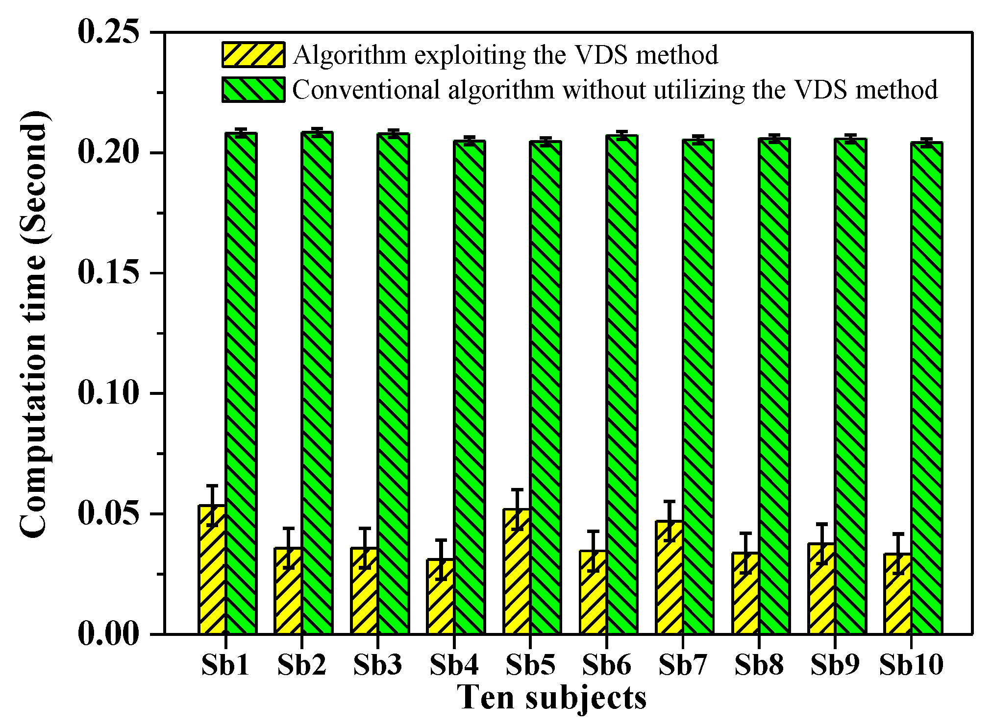
Finally, we further demonstrated the VDS method to accelerate the computation of ApEn in EEG signals. The EEG signals used were the ten subjects’ EEG signals in Figure 9. We calculated the ApEns by adopting two algorithms, one exploited the VDS method to accelerate the computation of the ApEn and the other was a conventional algorithm without utilizing the VDS method. Figure 14 shows the computation time of ApEn in the ten subjects’ EEG signals. The mean computation times are 0.0395 s and 0.206 s corresponding to the algorithm exploiting the VDS method and the conventional algorithm without exploiting VDS method, respectively. The computation time of ApEn is significantly (p < 0.005) reduced by utilizing the VDS method and the standard deviation of the computation time for the algorithm exploiting the VDS method is greater that for the conventional algorithm. These results indicate that the computation of ApEn can be greatly accelerated by exploiting the VDS method. The measurement values of ApEn by adoption of the two algorithms are identical.

Table 5. The measurement values of ApEn and SpEn in the ten subjects’ EEG signals. The computational parameters are N = 1000, m = 2, r = 0.2 × STD, where STD is the standard deviation of each EEG signal.

Subjects’ Label	SpEn	ApEn	Subjects’ Label	SpEn	ApEn
Sb1	1.12	1.12	Sb6	1.80	1.52
Sb2	1.52	1.43	Sb7	1.57	1.38
Sb3	1.32	1.30	Sb8	0.97	1.03
Sb4	1.40	1.35	Sb9	1.87	1.56
Sb5	1.36	1.24	Sb10	1.30	1.26

gives the measurement values of ApEn and SpEn in the ten subjects’ EEG signals.

There are some issues that need to be pointed out. The methods are implemented with MATLAB2016 (The Mathworks Inc., Natick, MA, USA) and run on an ordinary computer (Intel Core i7 CPU @ 3.2 GHz; 16 GB RAM; Windows 7). It is well-known that different programming languages and computing speeds of hardware can lead to different executing times. However, the changing trends of relative computation time of between the VDS method and the conventional method are consistent, no matter what kinds of programming language and hardware are used in experiment. Thus, the experimental conclusions with respect to time efficiency of computation by the VDS method are reliable.

There are some limitations to the VDS method. On one hand, the level of optimization of the computation time by the VDS method depends on the statistic property of the signal itself. The decision quantity, Decis(i,j), is defined as the absolute value of the sum of all components in vectors ${\mathit{X}}_i^{(m)}$ minus the sum of all components in vectors ${\mathit{X}}_j^{(m)}$ and has some kind of statistical characteristic. Only when the Decis(i,j) of arbitrary two vectors is greater than m × r can the computation time of entropy measures be optimized. On the other hand, for the VDS method, the time efficiency of computation by the VDS method may reach a certain limit. This fact can be observed from the experimental results in Section 3. For five kinds of EEG signals of different lengths, the time-reduced rate of computation of SpEn by the VDS method is about 82% compared with the conventional method. In practical applications, the longer the length of data, the greater the computation time. Thus, the computation time of SpEn may still be long for signals of long length, even though the VDS method is adopted.

Despite these limitations, the proposed VDS method is still considered to be promising. One advantage is that the VDS method may be jointly applied with other fast algorithms such as the existing SKD algorithm [21], recursive sample entropy algorithm [23] and so on, to further accelerate computation of entropy measures. There is no doubt that the proposed method is applicable to other entropy measures, such as ApEn and MSE. This implies a potential for extensive application, which is of important value.

4. Conclusions

In this study, we reported a reliable method capable of accelerating the computation of entropy measures such as ApEn, SpEn, TSME and so on. The experimental results demonstrate convincingly that the computation of entropy measures can be sped up by exploiting the VDS method. Taking advantage of the VDS method, the time-reduced rates of the computation of SpEn in random signals and EEG signals are low at 78.5% and 78.9%, respectively, compared with the conventional method. By quantitative analyses, we find that the percentage of vectors determined as being dissimilar by the VDS decision in the computation process is about 84.5% for the random signals and there is an average of 85.6% for the EEG signals. For EEG signals of different lengths (N = 500, N = 1000, N = 2000, N = 4000, N = 8000), the time-reduced rate of the computation of SpEn by the VDS method is about 80.1~82.8%. We further demonstrate the use of the VDS method for success in accelerating the computations of not only SpEn in EMG and ECG signals but also TSME and ApEn in EEG signals. We confirm that the VDS method is effective and practical for accelerating the computation of entropy measures and deem that it has promising applications in the area of biomedical informatics.

The Matlab codes with respect to the VDS method for accelerating computation of SpEn, the conventional method for computation of SpEn, the testing program for quantitative analysis and the VDS method for accelerating the computation of TSME are all available at the author’s personal homepage: https://sites.google.com/site/hitluyun/code/acemvds.

References

- Grandy, T.H.; Garrett, D.D.; Schmiedek, F.; Werkle-Bergner, M. On the estimation of brain signal entropy from sparse neuroimaging data. Sci. Rep. 2016, 6, 23073. [Google Scholar] [CrossRef] [PubMed]
- Cao, Y.; Cai, L.; Wang, J.; Wang, R.; Yu, H.; Cao, Y.; Liu, J. Characterization of complexity in the electroencephalograph activity of alzheimer’s disease based on fuzzy entropy. Chaos 2015, 25, 083116. [Google Scholar] [CrossRef] [PubMed]
- Arunkumar, N.; Ramkumar, K.; Venkatraman, V.; Abdulhay, E.; Fernandes, S.L.; Kadry, S.; Segal, S. Classification of focal and non focal EEG using entropies. Pattern Recognit. Lett. 2017, 94, 112–117. [Google Scholar]
- Su, C.; Liang, Z.; Li, X.; Li, D.; Li, Y.; Ursino, M. A comparison of multiscale permutation entropy measures in on-line depth of anesthesia monitoring. PLoS ONE 2016, 11, e0164104. [Google Scholar] [CrossRef] [PubMed]
- Liang, Z.; Wang, Y.; Sun, X.; Li, D.; Voss, L.J.; Sleigh, J.W.; Hagihira, S.; Li, X. EEG entropy measures in anesthesia. Front. Comput. Neurosci. 2015, 9, 16. [Google Scholar] [CrossRef] [PubMed]
- Patidar, S.; Panigrahi, T. Detection of epileptic seizure using Kraskov entropy applied on tunable-Q wavelet transform of EEG signals. Biomed. Signal Process. Control 2017, 34, 74–80. [Google Scholar] [CrossRef]
- Acharya, U.R.; Fujita, H.; Sudarshan, V.K.; Bhat, S.; Koh, J.E.W. Application of entropies for automated diagnosis of epilepsy using EEG signals: A review. Knowl.-Based Syst. 2015, 88, 85–96. [Google Scholar] [CrossRef]
- Li, X.; Jiang, Y.; Hong, J.; Dong, Y.; Yao, L. Estimation of cognitive workload by approximate entropy of EEG. J. Mech. Med. Biol. 2016, 16, 1650077. [Google Scholar] [CrossRef]
- Song, Y.; Zhang, J. Discriminating preictal and interictal brain states in intracranial EEG by sample entropy and extreme learning machine. J. Neurosci. Methods 2016, 257, 45–54. [Google Scholar] [CrossRef] [PubMed]
- Pincus, S.M. Approximate entropy as a measure of system complexity. Proc. Natl. Acad. Sci. USA 1991, 88, 2297–2301. [Google Scholar] [CrossRef] [PubMed]
- Li, P.; Liu, C.; Li, K.; Zheng, D.; Liu, C.; Hou, Y. Assessing the complexity of short-term heartbeat interval series by distribution entropy. Med. Biol. Eng. Comput. 2015, 53, 77–87. [Google Scholar] [CrossRef] [PubMed]
- Manis, G.; Aktaruzzaman, M.; Sassi, R. Bubble entropy: An entropy almost free of parameters. IEEE Trans. Biomed. Eng. 2017, 64, 2711–2718. [Google Scholar] [CrossRef] [PubMed]
- Lerga, J.; Saulig, N.; Lerga, R.; Milanović, Ž. Effects of TFD thresholding on EEG signal analysis based on the local Rényi entropy. In Proceedings of the 2nd International Multidisciplinary Conference on Computer and Energy Science SpliTech 2017, Split, Croatia, 12–14 July 2017; pp. 1–6. [Google Scholar]
- Lerga, J.; Saulig, N.; Lerga, R.; Štajduhar, I. TFD thresholding in estimating the number of EEG components and the dominant IF using the short-term Rényi Entropy. In Proceedings of the 10th International Symposium on Image and Signal Processing and Analysis—ISPA 2017, Ljubljana, Slovenia, 18–20 September 2017; pp. 80–85. [Google Scholar]
- Lerga, J.; Saulig, N.; Mozetič, V.; Lerga, R. Number of EEG signal components estimated using the short-term Rényi entropy. In Proceedings of the 1st International Multidisciplinary Conference on Computer and Energy Science SpliTech 2016, Split, Croatia, 13–15 July 2016; pp. 1–6. [Google Scholar]
- Richman, J.S.; Moorman, J.R. Physiological time-series analysis using approximate entropy and sample entropy. Am. J. Physiol. Heart Circ. Physiol. 2000, 278, H2039–H2049. [Google Scholar] [PubMed]
- Chen, W.; Wang, Z.; Xie, H.; Yu, W. Characterization of surface EMG signal based on fuzzy entropy. IEEE Trans. Neural Syst. Rehabil. Eng. 2007, 15, 266–272. [Google Scholar] [CrossRef] [PubMed]
- Costa, M.; Goldberger, A.L.; Peng, C.K. Multiscale entropy analysis of complex physiologic time series. Phys. Rev. Lett. 2002, 89, 068102. [Google Scholar] [CrossRef] [PubMed]
- Costa, M.; Goldberger, A.L.; Peng, C.K. Multiscale entropy analysis of biological signals. Phys. Rev. E 2005, 71, 021906. [Google Scholar] [CrossRef] [PubMed]
- Liang, Z.; Duan, X.; Li, X.L. Entropy measures in neural signals. In Signal Processing in Neuroscience; Li, X.L., Ed.; Springer: Singapore, 2016; pp. 125–166. ISBN 978-981-10-1822-0. [Google Scholar]
- Pan, Y.H.; Wang, Y.H.; Liang, S.F.; Lee, K.T. Fast computation of sample entropy and approximate entropy in biomedicine. Comput. Meth. Program Biomed. 2011, 104, 382–396. [Google Scholar] [CrossRef] [PubMed]
- Manis, G. Fast computation of approximate entropy. Comput. Meth. Programs Biomed. 2008, 91, 48–54. [Google Scholar] [CrossRef] [PubMed]
- Shohei, S.; Koichi, S.; Hiromitsu, O. Recursive sample-entropy method and its application for complexity observation of earth current. In Proceedings of the 2008 International Conference on Control, Automation and Systems (ICCAS 2008), Seoul, Korea, 14–17 October 2008; pp. 1250–1253. [Google Scholar]
- Hong, B.; Yang, F.; Tang, Q.; Tin-Cheung, C. Approximate entropy and its preliminary application in the field of EEG and cognition. In Proceedings of the 20th Annual International Conference of the IEEE Engineering in Medicine and Biology Society, Hong Kong, China, 29 October–1 November 1998; pp. 2091–2094. [Google Scholar]
- Bandt, C.; Pompe, B. Permutation entropy: A natural complexity measure for time series. Phys. Rev. Lett. 2002, 88, 174102. [Google Scholar] [CrossRef] [PubMed]
- Olofsen, E.; Sleigh, J.W.; Dahan, A. Permutation entropy of the electroencephalogram: A measure of anaesthetic drug effect. Br. J. Anaesth. 2008, 101, 810–821. [Google Scholar] [CrossRef] [PubMed]
- Wang, Y.; Xu, G.; Zhang, S.; Luo, A.; Li, M.; Han, C. EEG signal co-channel interference suppression based on image dimensionality reduction and permutation entropy. Signal Process. 2017, 134, 113–122. [Google Scholar] [CrossRef]
- Deng, B.; Liang, L.; Li, S.; Wang, R.; Yu, H.; Wang, J.; Wei, X. Complexity extraction of electroencephalograms in Alzheimer’s disease with weighted-permutation entropy. Chaos 2015, 25, 043105. [Google Scholar] [CrossRef] [PubMed]
- Azami, H.; Escudero, J. Improved multiscale permutation entropy for biomedical signal analysis: Interpretation and application to electroencephalogram recordings. Biomed. Signal Process. Control 2016, 23, 28–41. [Google Scholar] [CrossRef]
- Jian, Y.; Mao, D.; Xu, Y. A fast algorithm for computing sample entropy. Adv. Adapt. Data Anal. 2011, 3, 167–186. [Google Scholar] [CrossRef]
- Zurek, S.; Guzik, P.; Pawlak, S.; Kosmider, M.; Piskorski, J. On the relation between correlation dimension, approximate entropy and sample entropy parameters and a fast algorithm for their calculation. Phys. A Stat. Mech. Appl. 2012, 391, 6601–6610. [Google Scholar] [CrossRef]
- Wu, S.-D.; Wu, C.W.; Lee, K.Y.; Lin, S.G. Modified multiscale entropy for short-term time series analysis. Phys. A Stat. Mech. Appl. 2013, 392, 5865–5873. [Google Scholar] [CrossRef]
- Wu, S.D.; Wu, C.W.; Lin, S.G.; Wang, C.C.; Lee, K.Y. Time series analysis using composite multiscale entropy. Entropy 2013, 15, 1069–1084. [Google Scholar] [CrossRef]
- Pham, T.D. Time-shift multiscale entropy analysis of physiological signals. Entropy 2017, 19, 257. [Google Scholar] [CrossRef]
- Higuchi, T. Approach to an irregular time series on the basis of the fractal theory. Physica D 1988, 31, 277–283. [Google Scholar] [CrossRef]
- Lerga, J.; Saulig, N.; Mozetič, V. Algorithm based on the short-term Rényi entropy and IF estimation for noisy EEG signals analysis. Comput. Biol. Med. 2017, 80, 1–13. [Google Scholar] [CrossRef] [PubMed]
- Goldberger, A.L.; Amaral, L.A.N.; Glass, L.; Hausdorff, J.M.; Ivanov, P.C.; Mark, R.G.; Mietus, J.E.; Moody, G.B.; Peng, C.K.; Stanley, H.E. PhysioBank, PhysioToolkit and PhysioNet: Components of a New Research Resource for Complex Physiologic Signals. Circulation 2000, 101, e215–e220. [Google Scholar] [CrossRef] [PubMed]
- Lichman, M. UCI Machine Learning Repository. Available online: http://archive.ics.uci.edu/ml (accessed on 27 October 2017).
- Pham’s Personal Homepage. Available online: https://sites.google.com/site/professortuanpham/codes (accessed on 21 September 2017).
Figure 1.
Implementation of the vectors with dissimilarity (VDS) method for accelerating the computation of sample entropy (SpEn).
Figure 2.
The random signal of 1000 data points uniformly distributed in the interval (0, 1).
Figure 3.
(a) The computation time of SpEn in ten random signals using the VDS method and conventional method, the computation time of SpEn is significantly (p < 0.005) reduced using the VDS method; (b) The percentages of vectors determined to be dissimilar by the VDS decision, for the 10 random signals, the percentages are 84.7%, 84.3%, 84.5%, 84.7%, 84.5%, 84.9%, 85.1%, 84.0%, 85.1% and 84.7%, respectively, as determined by the VDS decision during computation.
Figure 4.
The sinusoidal signal and the mixed-signals with white noises of power −12 dBW, −6 dBW and 0 dBW, respectively.
Figure 5.
(a) The computation times of SpEn in the six mixed-signals using the VDS and conventional method; (b) The measurement values of SpEn in the sinusoidal signal and six mixed-signals.
Figure 6.
Electroencephalogram (EEG) signals of length N = 1000 from ten channels. The markers from GP1 to GP10 correspond to the ten different EEG signals. The vertical axis indicates the amplitude of the EEG signals.
Figure 7.
(a) The computation time of SpEn in the ten channels’ EEG signals of length N = 1000 using the VDS method and the conventional method, the computation time of SpEn is significantly (p < 0.005) reduced using the VDS method; (b) The percentages of vectors determined to be dissimilar by the VDS decision, for the ten channels’ EEG signals the percentages are 84.7%, 85.8%, 85.6%, 86.6%, 87.5%, 84.3%, 82.8%, 86.3%, 86.5% and 86.6%, respectively, as determined by the VDS decision in the computation process.
Figure 8.
(a) The changes in computation times of SpEn in the ten channels’ EEG signals over parameter β; (b) The mean computation time of SpEn in the ten channels’ EEG signals increases with the increase of the value of parameter m.
Figure 9.
EEG signals from ten different subjects corresponding to electrode name Cz (numbering 11 in the records). The markers from Sb1 to Sb10 correspond to different experimental subjects, labeled from S001 to S010.
Figure 10.
The computation time of SpEn in ten subjects’ EEG signals by adopting the VDS method and conventional method. The computational parameters are N = 1000, m = 2 and r = 0.2 × STD, where STD is the standard deviation of each EEG signal. The computation time of SpEn is significantly (p < 0.005) reduced using the VDS method.
Figure 11.
The electromyography (EMG) and electrocardiogram (ECG) signals.
Figure 12.
The computation times of SpEn in EMG and ECG signals using the VDS and conventional method, for the EMG and ECG signals the computation times of the VDS method are all significantly (p < 0.005) reduced using the VDS method. (a) The mean computation times of SpEn by adoption of the VDS and conventional method are 0.396 s and 1.848 s, respectively; (b) the mean computation times of SpEn by adoption of the VDS method and conventional method are 0.218 s and 0.892 s, respectively.
Figure 13.
EEG signals from ten different subjects corresponding to electrode name Fz (numbering 34 in the records). The markers from Sb1 to Sb10 correspond to different experimental subjects labeled from S001 to S010.
Figure 14.
The computation time of ApEn in the ten subjects’ EEG signals by the algorithm exploiting the VDS method and conventional algorithm without exploiting the VDS method. The computation time of ApEn is significantly (p < 0.005) reduced by exploiting the VDS method.