Model Order Reduction: A Comparison between Integer and Non-Integer Order Systems Approaches
by
 , ,
, ,
Riccardo Caponetto
1,* ,
,
José Tenreiro Machado
2 ,
,
Emanuele Murgano
1 and
Maria Gabriella Xibilia
3 1
Dipartimento di Ingegneria Elettrica Elettronica e Informatica, University of Catania, 95125 Catania, Italy
2
Institute of Engineering, Polytechnic of Porto, 4200-072 Porto, Portugal
3
Dipartimento di Ingegneria, University of Messina, 98121 Messina, Italy
*
Author to whom correspondence should be addressed.
Entropy 2019, 21(9), 876; https://0-doi-org.brum.beds.ac.uk/10.3390/e21090876
Submission received: 14 August 2019
/
Revised: 29 August 2019
/
Accepted: 6 September 2019
/
Published: 9 September 2019
(This article belongs to the Special Issue The Fractional View of Complexity)
Abstract
:In this paper, classical and non-integer model order reduction methodologies are compared. Non integer order calculus has been used to generalize many classical control strategies. The property of compressing information in modelling systems, distributed in time and space, and the capability of describing long-term memory effects in dynamical systems are two features suggesting also the application of fractional calculus in model order reduction. In the paper, an open loop balanced realization is compared with three approaches based on a non-integer representation of the reduced system. Several case studies are considered and compared. The results confirm the capability of fractional order systems to capture and compress the dynamics of high order systems.
1. Introduction
A relevant topic in automatic control is the Model Order Reduction (MOR). The MOR approximates a high-order Linear Time-Invariant (LTI) system with a low-order one, neglecting the less significant state-space variables, decreasing therefore the number of variables and parameters needed for its representation, and simplifying the controller design procedure. Other fields where the use of MOR is highly recommended are related to information compression applications and filters design.
Different strategies are presented in the literature, among which, in the case of asymptotically stable LTI systems, one of the most relevant is based on the open loop balanced realization [1]. Other techniques have been defined using either optimization algorithms such as Genetic Algorithm (GA) [2] and Particle Swarm Optimization [3], or using Artificial Neural Networks [4].
In parallel to these methods, new MOR strategies, see [5], have been investigated applying Fractional Order Calculus (FOC) [6], due to its capability for modelling complex physical phenomena with fractional differential equations. The strategy proposed in [5] looks at the norm of the error between the original and the approximated transfer function and it is restricted to systems with specific proprieties.
In this paper, a comparison between classical and fractional order MOR methodologies is presented. Different optimization algorithms, evolutionary and gradient based, have been applied for obtaining the fractional order reduced models. Suitable indexes for the approximation error in the frequency and time domains are considered. In particular, the open loop balanced realization is compared with three other procedures that provide fractional order reduced systems.
2. Some Notes on Fractional Calculus
The long-range temporal or spatial dependence phenomena inherent to fractional order systems present unique peculiarities, not supported by their integer order counterpart that allows for better models for the dynamics of complex processes. In many cases, these properties make fractional order systems more adequate than the standard integer order ones. Fractional (or non integer order) systems can be considered as a generalization of integer order formulation [6,7].
The integro-differential operator with as operation limits and is defined as follows:
To evaluate a fractional-order derivative or integral of a function, three different definitions are used: for continuous-time domain, these are the Riemann–Liouville (RL) and Caputo (C), while, in the discrete domain, the Grunwald-Letnikov (GL) [6,8].
The RL and C definitions for a time-varying function are defined, respectively, by:
and
where and is the Euler Gamma function [9].
The GL definition instead is given by:
where evaluates the integer part of its argument.
It is worth noticing that, using the Caputo definition, the initial conditions for fractional-order differential equations are in the same form as its integer-order counterpart, even if some adjustments are necessary [10].
Typical applications of FOC can be found in control [11,12,13,14,15,16,17,18,19,20], chaos [21], Fractional Order Element (FOE) [22,23,24,25,26], Fractional Order Impedance (FOI) characterization [27,28,29], and medical applications [30,31,32]. More recently, fractional calculus is being applied in the study of complex systems. The state of the art can be found in [33], where the broad impact of entropy and information theory-based techniques in complexity, nonlinearity, and fractionality has been shown. A further characterizing property of fractional systems is their capability to model systems with memory as in economy and finance [34,35]. Entropy is also investigated in the framework of the fractional calculus [36]. For example, in [37], a fractional order derivative was applied to the probability distribution function introducing a new perspective in entropy definition. In [38], the Rényi entropy, inspired in the concepts of fractional calculus, was compared with other fractional entropies showing a superior sensitivity to the characteristics exhibited by a distinct data set. Entropy, information theory and fractional calculus tools, have been also recently applied for studying the dynamics of a national soccer league. The complex system state, consisting of the goals scored by the teams, is processed by means of different tools, namely entropy, mutual information and Jensen–Shannon divergence [39].
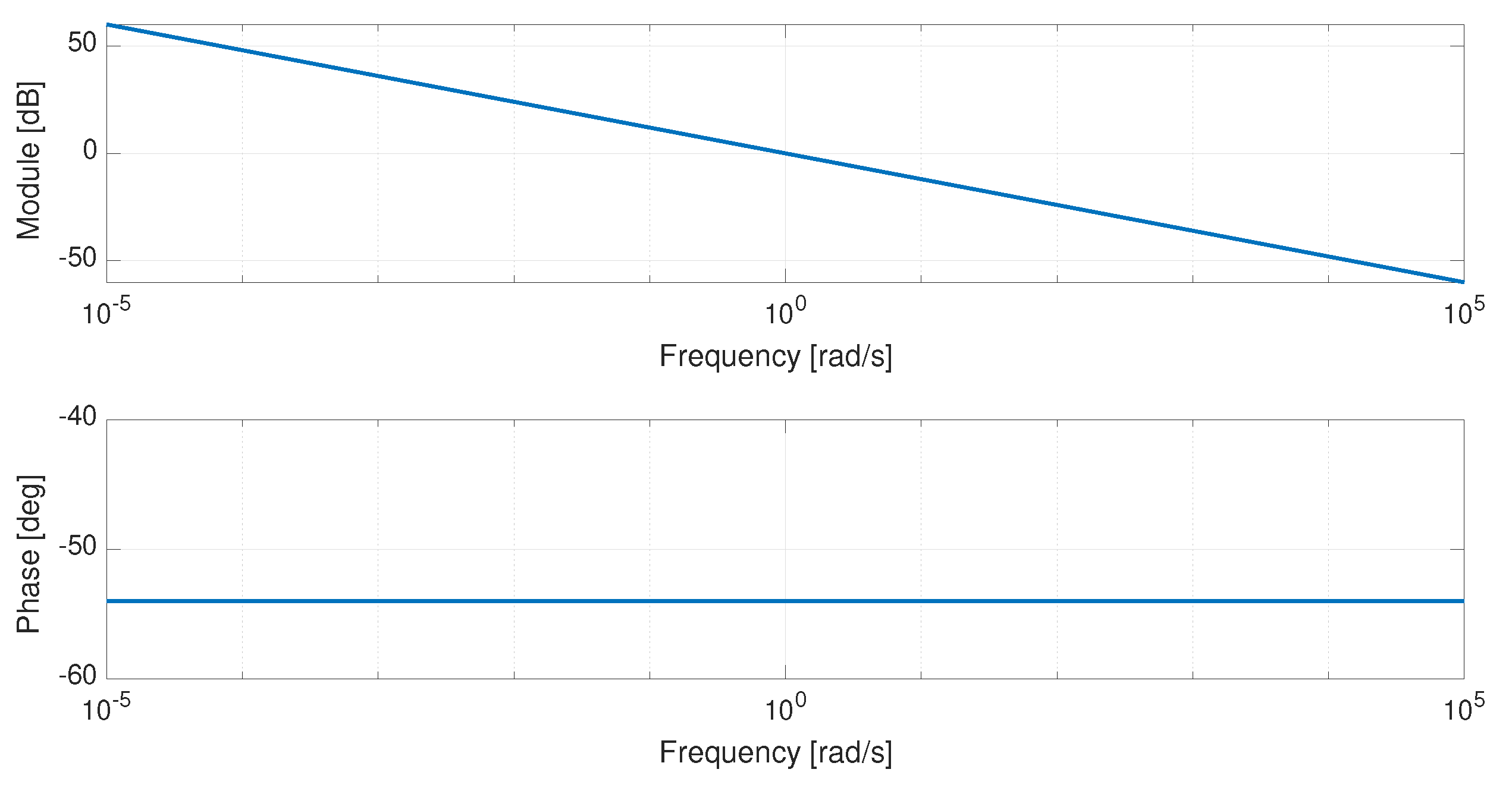
For a fractional order system, it is possible to define the Laplace transform—see [6]. The most common example of fractional-order system is the fractional-order integrator:
where .
As it is possible to observe in Figure 1, the behaviour of the fractional-order integrator is different from that of the integer order one. Evaluating module and phase of Equation (5), it follows that the module is equal to dB/dec, while the phase is constant in all the frequency domain and equal to . In the example, with , the module has a slope of dB/dec, whereas the phase is constant to . Therefore, selecting only one parameter, it is possible to obtain different dynamics. This property can be useful both in control and in system modelling.
3. Description of the Investigated MOR Techniques
In this section, the four different methodologies are presented and briefly discussed.
3.1. Open-Loop Balancing Reduction
The open-loop balancing reduction is one of the most relevant techniques used to reduce the model order of a LTI system because it deals directly with the state variables, evaluating the less significant state variables on the basis of their energy contribution. This technique was proposed in [1] and it is valid for asymptotically stable systems.
Given an LTI asymptotically stable system, with state-space matrices , completely controllable and observable, it is possible to define two matrices, namely the controllability and observability Gramians, and , respectively. These two matrices are positive definite and symmetrical. The singular values of the controllability Gramian are equal to those of the observability one and their product is a invariant system. The matrices can be evaluated as solutions of the following Lyapunov equations:
where Equations (6a) and (6b) are the controllability and observability Gramian equations, respectively. The practical computation of Gramian matrices for FOC-LTIs has been recently discussed in [40].
The system singular values are defined as the eigenvalues of the product of the two Gramians and play a fundamental role in the open-loop balancing reduction. In fact, it is possible to determine a particular representation where that is, where they are coincident and equal to a diagonal matrix, with values that are the square root of the system singular values. This representation is called Open Loop Balanced Realization (OLBR) [41] and allows us to analyse both the controllability and observability of the system looking at the same parameters and to select strong and weak observable and controllable state-space variables. Since the system singular values refer to state-space variables energy, if appropriately sorted, they allow neglecting the states whose contributions are less significant. In this way, model order reduction can be performed.
Assuming that the system under investigation is asymptotically stable, completely observable and controllable and represented in the OLBR form, if a singular value exists such that , then two clusters can be defined: the first one that represents the strongest controllable and observable variables, and the second one corresponding to the weakest ones. The system can be decomposed in the following way:
where and , correspond to the strongest and weakest controllable and observable state-space variables, respectively. If the direct truncation method is applied, then the equivalent reduced system will be the following one, supposing :
It means that the weakest part is neglected setting .
In the following, this method will be labelled with Method in [1], according to the related reference number.
3.2. Implicit Model Order Reduction via Fractional Order Calculus
In this section, the implicit model order reduction introduced in [5] is reported. The method differs from the open-loop balancing reduction because it deals with the system representation via transfer function instead of state-space matrices. The system transfer function must have all poles and zeros real and negative, and assumes the following form:
where , and K are the zeros, poles and gain of the system.
The system modelled in Equation (10) is reduced via the following implicit model:
where is the transitional frequency and is the integration order. As a first step of the model reduction, the poles and zeros are organized into two vectors, sorted in increasing order, respectively and and a unique vector is built. Defining the minimum number of parameters to be used in the compression, all possible combinations with at least elements are extracted from S. All of these vectors must have a zero in the even index and a pole in the odd one. Furthermore, the first and the last elements must be poles. The reduced system will be chosen starting from these combination and defining and according to the procedure introduced in [5]. The implicit model approach requires that the system must have the first pole smaller than the first zero; only a pair of complex conjugate poles and the poles and zeroes must be real and negative.
In the following, this method will be labelled with Method [5], according to the related reference number.
3.3. Fractional Order Transfer Function Fitting
The third approach starts from the choice of one of the following approximation functions:
where A, B and C are real constants.
Equations (12a) and (12b) can be chosen to obtain a fractional order approximation of an integer order system characterized by a low-pass behaviour. Equation (12c) can model not only low-pass systems, but also systems with more zeros because or can assume negative values. Finally, in Equation (12d), a first integer order term is added if the fractional order term is not sufficient to model the system behaviour.
After choosing the approximating function, two optimization procedures are applied, and compared to determine the coefficients of the approximation. In particular, the Genetic Algorithms [42] and the fminsearch [43] procedures are compared. Numerical stimulations were performed by using routines and procedures given in [44,45].
Given N samples of the Interger Order Transfer Function (IOTF), , and having specified the desired frequency window for the approximation, a reduced Fractional Order Transfer Funtion (FOTF), , is chosen and the following cost function c:
is minimized to determine the FOTF parameters.
In Equation (13), the sum of each term is evaluated and then averaged with respect to the number of samples. The optimization based on the GAs will be referred to as a Fractional Order Genetic Algorithm FO-GA, while the other one with Fractional Order FMINS FO-FMINS. The fminsearch approach, when converging to the minimum, reveals sensitivity of the choice of the initial conditions. In order to overcome this problem in the applied FO-FMINS, the initial conditions are chosen as the mean value of the domain interval defined in the GA, while in a further step the FO-FMINS algorithm is applied five times defining the initial conditions for the next iteration as the identified parameters x of the previous iteration, i.e., .
The parameters adopted for the GAs optimization are reported in Table 1.
4. Numerical Examples
In this section, three different IOTFs taken from literature [2,5,41], see Table 2, are considered, and, for each of them, the aforementioned techniques are applied in the frequency range f= Hz. The comparison analysis is performed fixing the same number of parameters for all the four different reduced models, minimizing the error given in Equation (13).
4.1. System with Transfer Function
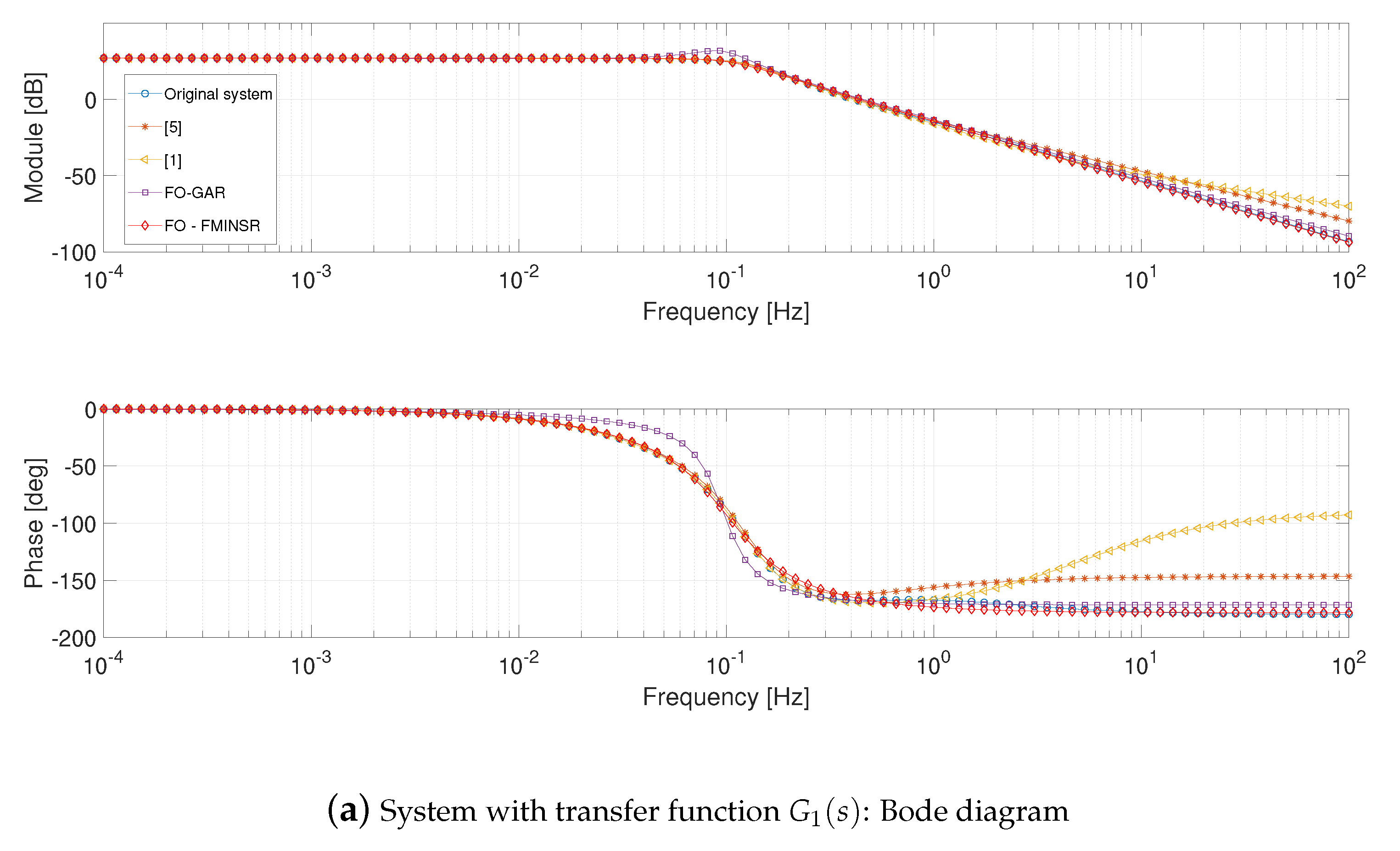
Considering the system, the frequency responses of the reduced models, see Figure 2a, show a better approximation in the cases of the two methodologies FO-GA and FO-FMINS. The approximating transfer functions are in the form of Equation (12c) for the FO-GA approach and in the form Equation (12d) for the FO-FMINS. Independently from the optimization algorithm and from the chosen approximating function, the fractional order models reveal themselves to be quite versatile in the approximation.
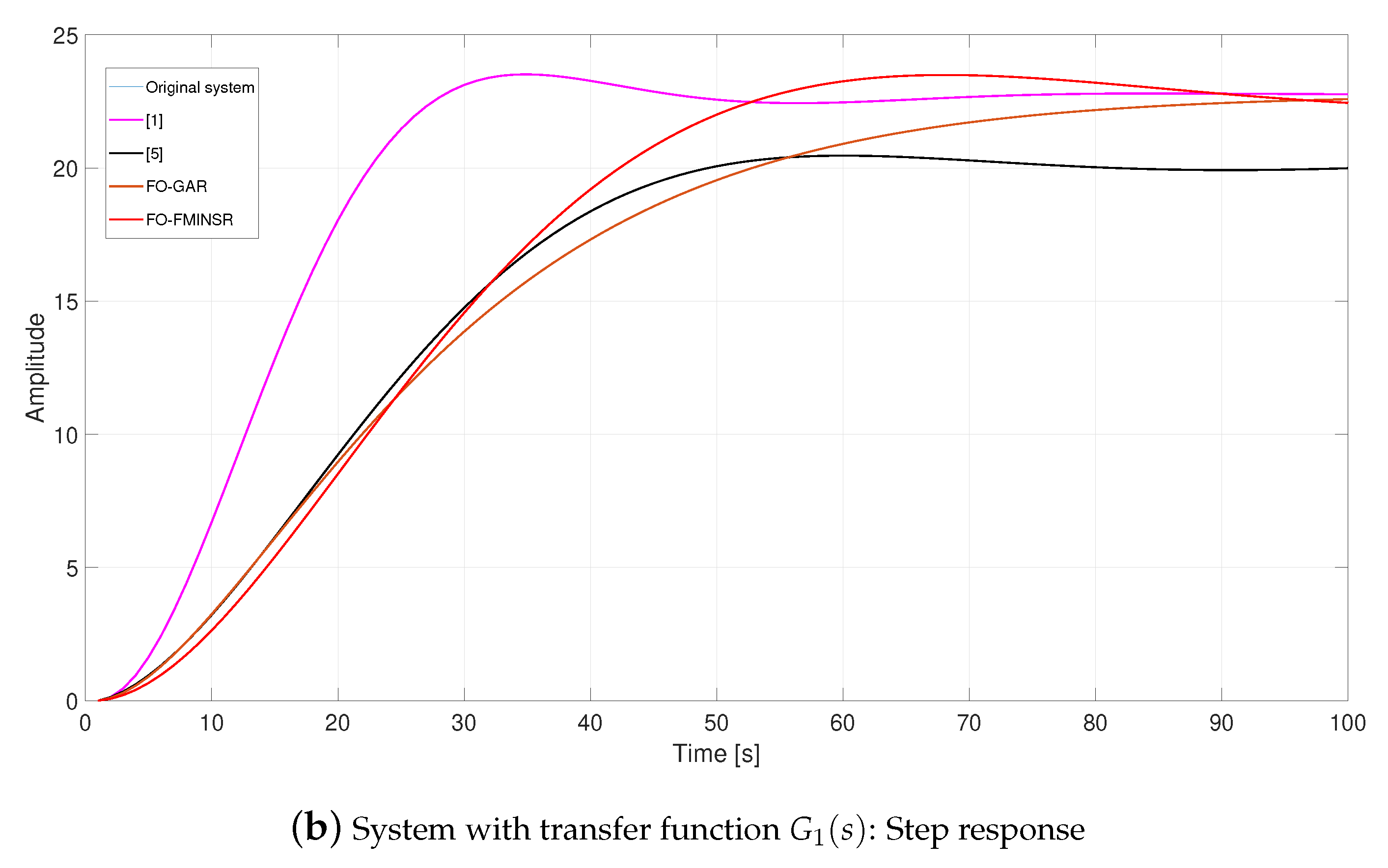
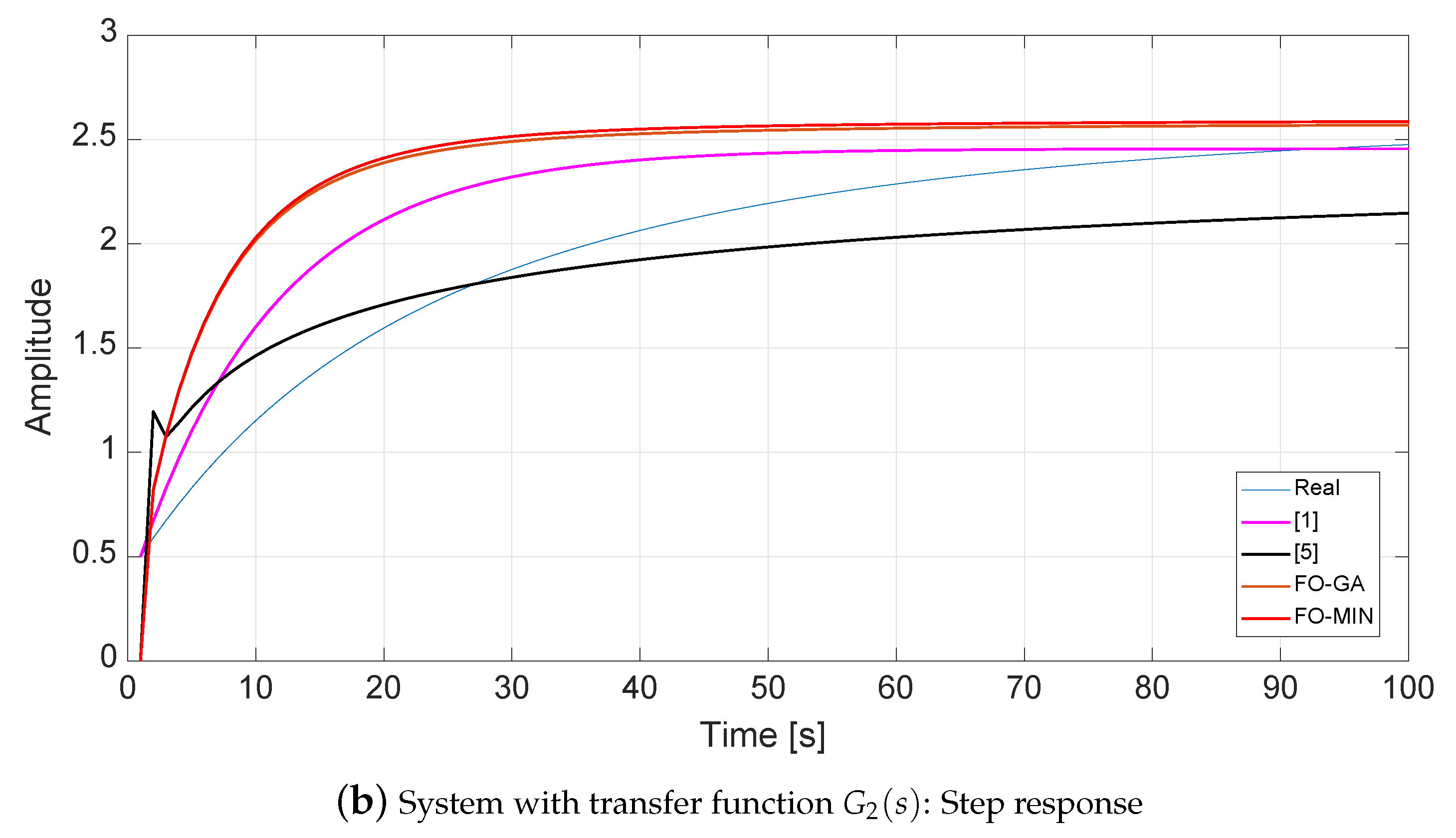
If the step responses are considered, see Figure 2b, it is possible to note that the worst performance is given by the implicit method in [5]. The reductions FO-GA and FO-FMINS provide the same steady state condition, while the best approximation is achieved by applying the balanced realization in [1]. The performance degradation in the step responses of FO-GA and FO-FMINS is due to the fact that the error function takes into account only the frequency domain responses.
4.2. System with Transfer Function
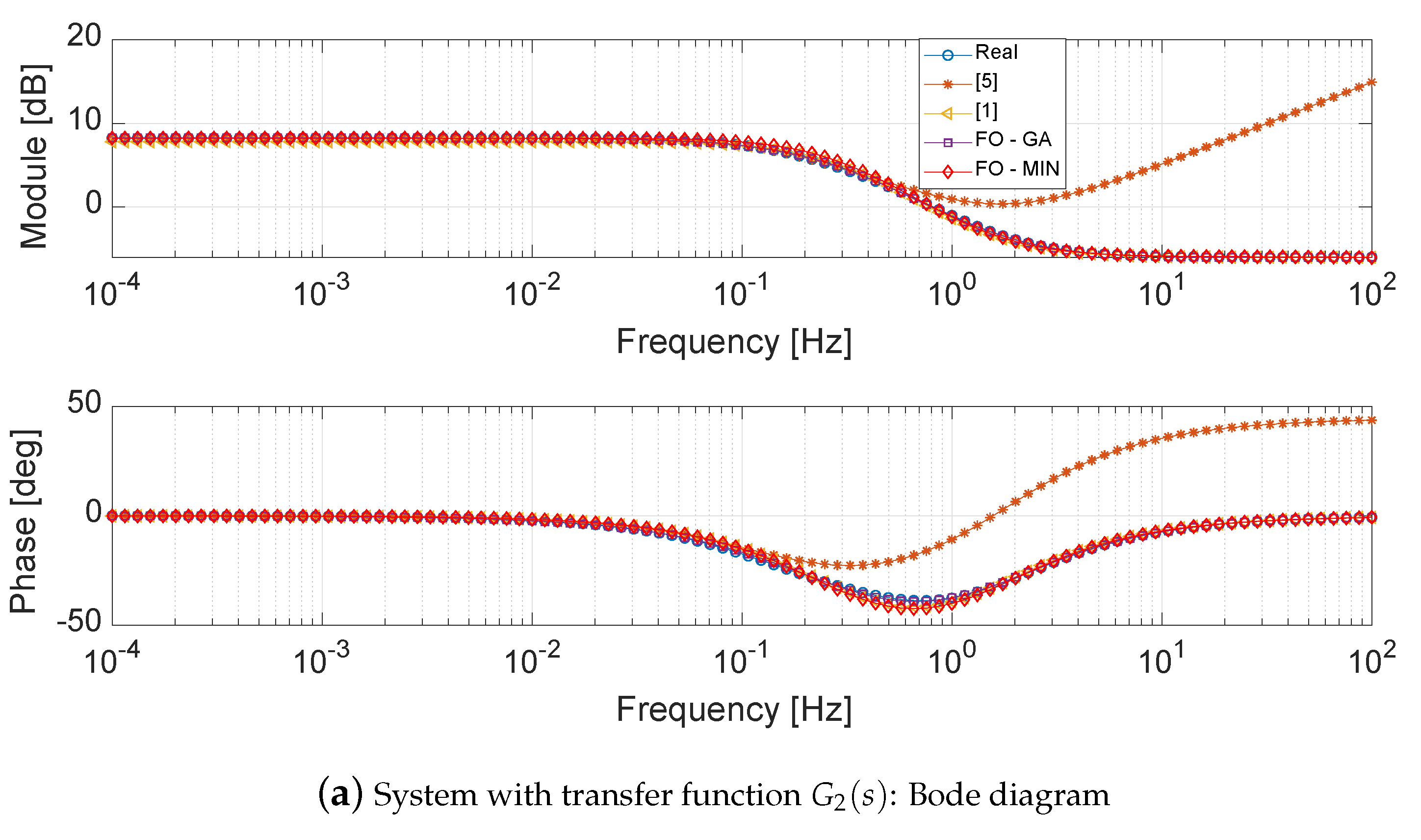
The transfer function represents an improper system. In the case of the implicit model [5], a zero of could not be taken into account in the reduction. In fact, in the vector S (see Section 3.2), the first and last position elements must be poles. Therefore, one zero will remain out of the approximation. The effect of the zero will start from the fourth decade, see Figure 3a, with the visible increase of the module and phase in the frequency approximation. On the contrary, the FO-GA approach is able to reduce the original system using a reduced improper transfer function with six parameters. In particular, the two parameters and bring to a reduced system in an improper form. The same consideration can be done for the FO-FMINS because, with , and neglecting , the reduced system is also in an improper form. The best approximation is provided by the balanced approach [1] that provides a simple and effective first order reduced model.
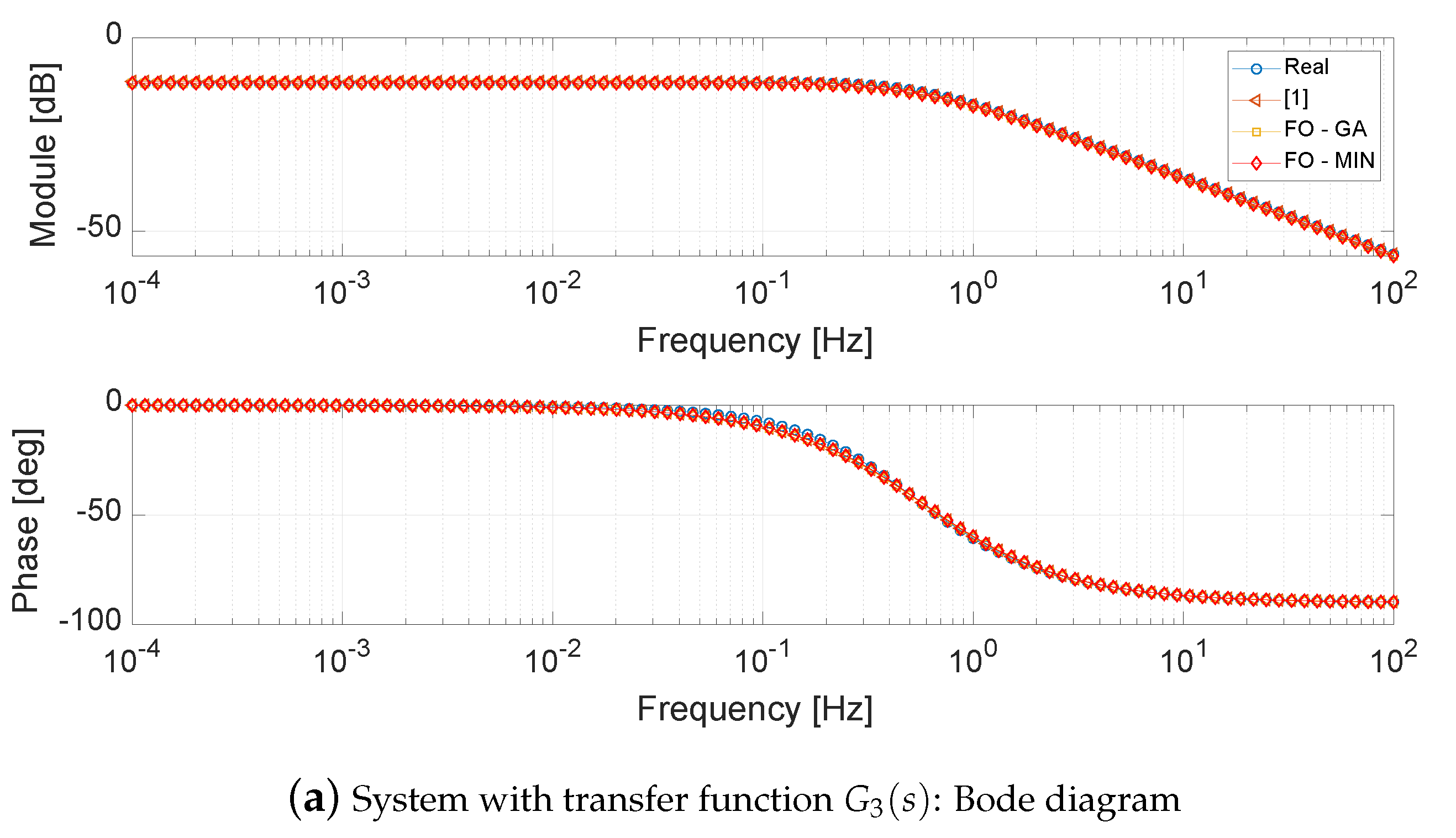
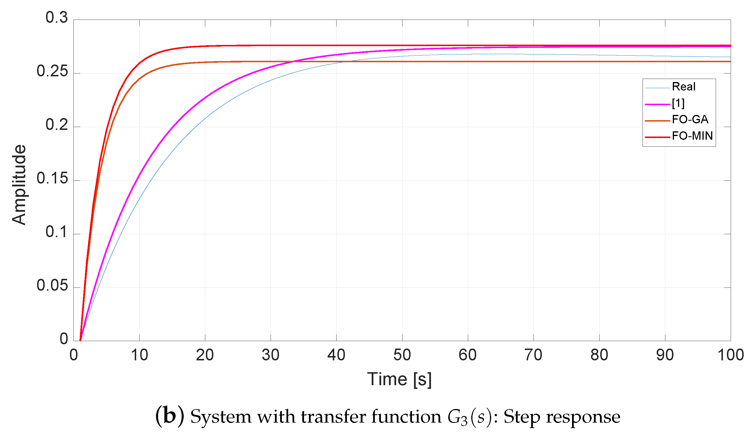
4.3. System with Transfer Function
With respect to system , it is possible to note that the implicit method [5] cannot be applied because the system has only one zero whose value is lower than the smaller pole. Looking at the frequency response, see Figure 4a, it is possible to see that the three methods are almost equivalent, guaranteeing the same performances in the frequency domain. On the other hand, by analysing the step responses shown in Figure 4b, it is possible to note that, during the transient, the response of the system was reduced by means of the balancing-based approach is very close to the response of the original system, while, in the steady state, the minimum error is obtained with the FO-GA approach.
5. Conclusions
In the previous section, a number of MOR techniques, based on integer and non-integer order models, was evaluated on four systems. Looking at the approximation error values, it can be observed that the techniques based on optimization algorithms are able to fit the IOTFs with good results.
Another important result is that, when dealing with state-space variables, the method [1] works better because the system energy is directly evaluated during the MOR, while this kind of analysis cannot be performed for the fractional order models [10].
In particular, the fminsearch optimization algorithm requires more iterations due to its high dependency on initial conditions, while the GAs do not suffer from this problem if the parameter ranges are well defined. On the contrary, the FO-R does not depend on them but on other constraints linked to system structure. The step responses show that the reduced model with fractional-order optimization algorithms achieve good results at the steady state. Further analysis will be performed looking at some system proprieties in order to find, if it exists, a class of transfer functions for which fractional-order based model reduction gives better results than [1]. Another interesting point is the definition of performance indices that also takes into account the time domain behaviour, see [46]. Future research activities will be devoted to the pseudo state space description [10] in fractional reduced order system.
Author Contributions
Conceptualization, R.C., J.T.M., E.M. and M.G.X.; methodology, R.C., J.T.M., E.M. and M.G.X.; software, E.M.; writing–original draft preparation, R.C., J.T.M., E.M. and M.G.X.; writing–review and editing, J.T.M.
Funding
This research received no external funding.
Acknowledgments
This work was supported by EU COST Action CA15225 “Fractional order systems: analysis, synthesis and their importance for future design”.
Conflicts of Interest
The authors declare no conflict of interest.
Abbreviations
The following abbreviations are used in this manuscript:
| MOR | Model Order Reduction |
| FOC | Fractional Order Calculus |
| GA | Genetic Algorithm |
| IOTF | Integer Order Transfer Function |
| Order of Differentiation | |
| FOS | Fractional Order System |
| FOTF | Fractional Order Transfer Function |
| OLBR | Open Loop Balancing Realization |
References
- Moore, B. Principal component analysis in linear systems: Controllability, observability, and model reduction. IEEE Trans. Automatic Control 1981, 26, 17–32. [Google Scholar] [CrossRef]
- Das, S.; Patnaik, P.; Jha, R. Model Order Reduction of High Order LTI System using Genetic Algorithm. In Proceedings of the 2017 International Conference on Computer, Communications and Electronics (Comptelix), Jaipur, India, 1–2 July 2017; pp. 73–77. [Google Scholar]
- Khaled, S. A generic model order reduction technique based on Particle Swarm Optimization (PSO) algorithm. In Proceedings of the IEEE EUROCON 2017—17th International Conference on Smart Technologies, Ohrid, Macedonia, 6–8 July 2017; pp. 193–196. [Google Scholar]
- Ahmed, A.; Khaled, S. Model order reduction using artificial neural networks. In Proceedings of the 2016 IEEE International Conference on Electronics, Circuits and Systems (ICECS), Monte Carlo, Monaco, 11–14 December 2016; pp. 89–92. [Google Scholar]
- Rachid, M.; Maamar, B.; Said, D. Approximation of high order integer systems by fractional order reduced parameter models. Math. Comput. Model. 2010, 51, 53–62. [Google Scholar]
- Oldham, K.B.; Spanier, J. The Fractional Calculus: Theory and Applications of Differentiation and Integration to Arbitrary Order; Elsevier Science: Amsterdam, The Netherlands, 1974. [Google Scholar]
- Ross, B. Fractional Calculus and its Applications; Springer: Berlin, Germay, 1975. [Google Scholar]
- Podlubny, I. Fractional Differential Equations. An Introduction to Fractional Derivatives, Fractional Differential Equations, Some Methods of Their Solution and Some of Their Applications; Academic Press: Cambridge, MA, USA, 1999. [Google Scholar]
- Sebah, P.; Gourdon, X. Introduction to the Gamma Functions. 2012. Available online: http://numbers.computation.free.fr/Constants/constants.html (accessed on 15 July 2019).
- Sabatier, J.; Farges, C.; Trigeassou, J.C. Fractional systems state space description: some wrong ideas and proposed solutions. J. Vib. Control 2014, 20, 1076–1084. [Google Scholar] [CrossRef]
- Podlubny, I. Fractional-order systems and PIλDμ controllers. IEEE Trans. Autom. Control 1999, 44, 208–214. [Google Scholar] [CrossRef]
- Caponetto, R.; Dongola, G.; Pappalardo, F.; Tomasello, V. Auto-Tuning and Fractional Order Controller Implementation on Hardware in the Loop System. J. Optim. Theory Appl. 2013, 156, 141–152. [Google Scholar] [CrossRef]
- Caponetto, R.; Dongola, G.; Maione, G.; Pisano, A. Integrated technology fractional order proportional- integral-derivative design. J. Vib. Control 2014, 20, 1066–1075. [Google Scholar] [CrossRef]
- De Keyser, R.; Muresan, C.; Ionescu, C. A novel auto-tuning method for fractional order PI/PD controllers. ISA Trans. 2016, 62, 268–275. [Google Scholar] [CrossRef]
- Caponetto, R.; Dongola, G. A numerical approach for computing stability region of FO-PID controller. J. Frankl. Inst. 2013, 350, 871–889. [Google Scholar] [CrossRef]
- Caponetto, R.; Dongola, G. Field programmable analog array implementation of noninteger order PIλDμ controller. J. Comput. Nonlinear Dyn. 2008, 3, 021302. [Google Scholar] [CrossRef]
- Caponetto, R.; Maione, G.; Pisano, A.; Rapaic, M.; Usai, E. Analysis and shaping of the self-sustained oscillations in relay controlled fractional-order systems. Fract. Calc. Appl. Anal. 2013, 16, 93–108. [Google Scholar] [CrossRef]
- Lino, P.; Maione, G. Design and simulation of fractional-order controllers of injection in CNG engines. IFAC Proc. Vol. 2013, 1, 582–587. [Google Scholar] [CrossRef]
- Caponetto, R.; Sapuppo, F.; Tomasello, V.; Maione, G.; Lino, P. Fractional-Order Identification and Control of Heating Processes with Non-Continuous Materials. Entropy 2016, 18, 398. [Google Scholar] [CrossRef]
- Coronel-Escamilla, A.; Gómez-Aguilar, J.; Torres, L.; Escobar-Jimènez, R.; Olivares-Peregrino, V. Fractional observer to estimate periodical forces. ISA Trans. 2018, 82, 30–41. [Google Scholar] [CrossRef] [PubMed]
- Petras, I. Fractional-Order Nonlinear Systems: Modeling, Analysis and Simulation; Springer: Berlin/Heidelberg, Germany, 2011. [Google Scholar]
- Mondal, D.; Biswas, K. Packaging of Single-Component Fractional Order Element. IEEE Trans. Device Mater. Reliab. 2013, 13, 73–80. [Google Scholar] [CrossRef]
- Jesus, I.; Machado, T. Development of fractional order capacitors based on electrolyte processes. Nonlinear Dyn. 2009, 56, 45–55. [Google Scholar] [CrossRef]
- Caponetto, R.; Dongola, G.; Fortuna, L.; Graziani, S.; Strazzeri, S. A fractional model for IPMC actuators. In Proceedings of the 2008 IEEE Instrumentation and Measurement Technology Conference, Victoria, BC, Canada, 12–15 May 2008; pp. 2103–2107. [Google Scholar]
- John, D.; Banerjee, S.; Bohannan, G.; Biswas, K. Solid-state fractional capacitor using MWCNT-epoxy nanocomposite. Appl. Phys. Lett. 2017, 110, 163504. [Google Scholar] [CrossRef]
- Buscarino, A.; Caponetto, R.; Di Pasquale, G.; Fortuna, L.; Graziani, S.; Pollicino, A. Carbon Black based capacitive Fractional Order Element towards a new electronic device. AEU—Int. J. Electron. Commun. 2018, 84, 307–312. [Google Scholar] [CrossRef]
- Said, L.; Radwan, A.; Madian, A.; Solimane, A. Fractional order oscillators based on operational transresistance amplifiers. AEU—Int. J. Electron. Commun. 2015, 69, 988–1003. [Google Scholar] [CrossRef]
- Krishna, S.; Das, S.; Biswas, K.; Goswami, B. Fabrication of a Fractional Order Capacitor With Desired Specifications: A Study on Process Identification and Characterization. IEEE Trans. Electron. Device 2011, 58, 4067–4072. [Google Scholar] [CrossRef]
- Bohannan, G. Electrical Component with Fractional Order Impedance. U.S. Patent n.20060267595, 30 November 2006. [Google Scholar]
- Vastarouchas, C.; Tsirimokou, G.; Freeborn, T.; Psychalinos, C. Emulation of an electrical-analogue of a fractional-order human respiratory mechanical impedance model using OTA topologies. AEU—Int. J. Electron. Commun. 2017, 78, 201–208. [Google Scholar] [CrossRef]
- Ionescu, C.; Machado, T.; De Keyser, R. Modeling of the lung impedance using a fractional-order ladder network with constant phase elements. IEEE Trans. Biomed. Circuits Syst. 2011, 5, 83–89. [Google Scholar] [CrossRef] [PubMed]
- Solís-Péreza, J.; Gómez-Aguilar, J.; Torres, L.; Escobar-Jiménez, R.; Reyes-Reyes, J. Fitting of experimental data using a fractional Kalman-like observer. ISA Trans. 2019, 88, 153–169. [Google Scholar] [CrossRef] [PubMed]
- Lopes, A.M.; Machado, T. Complex Systems and Fractional Dynamics. Entropy 2018, 20, 507. [Google Scholar] [CrossRef]
- Tarasov, V.; Tarasova, V. Criterion of Existence of Power-Law Memory for Economic Processes. Entropy 2018, 20, 414. [Google Scholar] [CrossRef]
- Mata, M.; Machado, J. Entropy Analysis of Monetary Unions. Entropy 2017, 19, 6245. [Google Scholar] [CrossRef]
- Machado, J. Fractional Order Generalized Information. Entropy 2014, 16, 2350–2361. [Google Scholar] [CrossRef] [Green Version]
- Karci, A. Fractional order entropy: New perspectives. Optik 2016, 27, 9172–9177. [Google Scholar] [CrossRef]
- Machado, T.; Lopes, A. Fractional Rényi entropy, Fractional Rényi entropy. Eur. Physic J. Plus 2019. [Google Scholar] [CrossRef]
- Lopes, A.; Machado, J. Entropy analysis of soccer dynamics. Entropy 2019, 21, 2. [Google Scholar] [CrossRef]
- Garrappa, R.; Popolizio, M. Computing the Matrix Mittag-Leffler Function with Applications to Fractional Calculus. J. Sci. Comput. 2018, 77, 129–153. [Google Scholar] [CrossRef] [Green Version]
- Fortuna, L.; Frasca, M. Optimal and Robust Control: Advanced Topics with MATLAB®; CRC-Press: Boca Raton, FL, USA, 2012. [Google Scholar]
- Goldberg, D. Genetic Algorithms in Search, Optimization, and Machine Learning; Addison-Wesley Professional: Boston, MA, USA, 1989. [Google Scholar]
- Lagarias, J.C.; Reeds, J.A.; Wright, M.H.; Wright, P.E. Convergence Properties of the Nelder-Mead Simplex Method in Low Dimensions. SIAM J. Optim. 1998, 9, 112–147. [Google Scholar] [CrossRef]
- Garrappa, R. Trapezoidal methods for fractional differential equations: Theoretical and computational aspects. Math. Comput. Simul. 2015, 110, 96–112. [Google Scholar] [CrossRef]
- Tepljakov, A.; Petlenkov, E.; Belikov, J. FOMCON: Fractional-order modeling and control toolbox for MATLAB. In Proceedings of the 18th International Conference Mixed Design of Integrated Circuits and Systems—MIXDES 2011, Gliwice, Poland, 16–18 June 2011; pp. 684–689. [Google Scholar]
- Garrappa, R.; Maione, G. Model order reduction on Krylov subspaces for fractional linear systems. IFAC Proc. Vol. 2013, 46, 143–148. [Google Scholar] [CrossRef]
Figure 1.
Bode diagram of .

Figure 2.
Bode diagram and step response of system with transfer function and corresponding fitted systems.
Figure 2.
Bode diagram and step response of system with transfer function and corresponding fitted systems.


Figure 3.
Bode diagram and step response of system with transfer function and corresponding fitted systems.
Figure 3.
Bode diagram and step response of system with transfer function and corresponding fitted systems.


Figure 4.
Bode diagram and step response of system with transfer function and corresponding fitted systems.
Figure 4.
Bode diagram and step response of system with transfer function and corresponding fitted systems.


Table 1.
GA parameters.
| Parameter | Value |
|---|---|
| Number of individuals | 3000 |
| Maximum number of generation | 150 |
| Generation gap | |
| Precision | 40 |
Table 2.
IOTF to be reduced.
| System | Transfer Function |
|---|---|
Table 3.
Errors amomg full and reduces order systems.
| System | Method in [1] | Method in [5] | FO-GA | FO-FMINS | No. of param. |
|---|---|---|---|---|---|
| [6,6,6,6] | |||||
| [2,4,6,5] | |||||
| not applicable | [2,-,2,2] |
© 2019 by the authors. Licensee MDPI, Basel, Switzerland. This article is an open access article distributed under the terms and conditions of the Creative Commons Attribution (CC BY) license (http://creativecommons.org/licenses/by/4.0/).
Share and Cite
MDPI and ACS Style
Caponetto, R.; Machado, J.T.; Murgano, E.; Xibilia, M.G. Model Order Reduction: A Comparison between Integer and Non-Integer Order Systems Approaches. Entropy 2019, 21, 876. https://0-doi-org.brum.beds.ac.uk/10.3390/e21090876
AMA Style
Caponetto R, Machado JT, Murgano E, Xibilia MG. Model Order Reduction: A Comparison between Integer and Non-Integer Order Systems Approaches. Entropy. 2019; 21(9):876. https://0-doi-org.brum.beds.ac.uk/10.3390/e21090876
Chicago/Turabian StyleCaponetto, Riccardo, José Tenreiro Machado, Emanuele Murgano, and Maria Gabriella Xibilia. 2019. "Model Order Reduction: A Comparison between Integer and Non-Integer Order Systems Approaches" Entropy 21, no. 9: 876. https://0-doi-org.brum.beds.ac.uk/10.3390/e21090876
Note that from the first issue of 2016, this journal uses article numbers instead of page numbers. See further details here.