A Dual Measure of Uncertainty: The Deng Extropy


1
Dipartimento di Matematica e Applicazioni “Renato Caccioppoli”, Università degli Studi di Napoli Federico II, I-80126 Naples, Italy
2
Dipartimento di Biologia, Università degli Studi di Napoli Federico II, I-80126 Naples, Italy
*
Author to whom correspondence should be addressed.
Entropy 2020, 22(5), 582; https://0-doi-org.brum.beds.ac.uk/10.3390/e22050582
Submission received: 6 May 2020
/
Revised: 17 May 2020
/
Accepted: 19 May 2020
/
Published: 21 May 2020
(This article belongs to the Section Information Theory, Probability and Statistics)
Abstract
:The extropy has recently been introduced as the dual concept of entropy. Moreover, in the context of the Dempster–Shafer evidence theory, Deng studied a new measure of discrimination, named the Deng entropy. In this paper, we define the Deng extropy and study its relation with Deng entropy, and examples are proposed in order to compare them. The behaviour of Deng extropy is studied under changes of focal elements. A characterization result is given for the maximum Deng extropy and, finally, a numerical example in pattern recognition is discussed in order to highlight the relevance of the new measure.
1. Introduction
Let X be a discrete random variable with support and with probability mass function vector . The Shannon entropy of X is defined as
where log is the natural logarithm, see [1]. It is a measure of information and discrimination about the uncertainty related to the random variable X. Lad et al. [2] proposed the extropy as the dual of entropy. This is a measure of uncertainty related to the outside and is defined as
Lad et al. proved the following property related to the sum of the entropy and the extropy:
where are the entropy and the extropy of a discrete random variable of which the support has cardinality two and the probability mass function vector is .
Dempster [3] and Shafer [4] introduced a method to study uncertainty. Their theory of evidence is a generalization of the classical probability theory. In D-S theory, an uncertain event with a finite number of alternatives is considered, and a mass function over the power set of the alternatives (i.e., a degree of confidence to all of its subsets) is defined. If we give positive mass only to singletons, a probability mass function is obtained. D-S theory allows us to describe more general situations in which there is less specific information.
Here we describe an example studied in [5] to explain how D-S theory extends the classical probability theory. Consider two boxes, A and B such that in A there are only red balls, whereas in B there are only green balls and the number of balls in each box is unknown. A ball is picked randomly from one of these two boxes. The box A is selected with probability and box B is selected with probability . Hence, the probability of picking a red ball is 0.6, , whereas the probability of picking a green ball is 0.4, . Suppose now that in box B there are green and red balls with rates unknown. The box A is still selected with probability and the box B with probability . In this case, we can not obtain the probability of picking a red ball. To analyze this problem, we can use D-S theory to express the uncertainty. In particular, we choose a mass function m such that, and .
Dempster–Shafer theory of evidence has several applications due to its advantages in dealing with uncertainty; for example, it is used in decision making [6,7], in risk evaluation [8,9], in reliability analysis [10,11] and so on. In the following, we recall the basic notions of this theory.
Let X be a frame of discernment, i.e., a set of mutually exclusive and collectively exhaustive events indicated by . The power set of X is indicated by and it has cardinality . A function is called a mass function or a basic probability assignment (BPA) if
If implies then m is also a probability mass function, i.e., BPAs generalize discrete random variables. Moreover, elements A such that are called focal elements. Given a BPA, we can evaluate for each focal element the pignistic probability transformation (PPT). Let us recall that the pignistic probability is the probability that a thinking being would assign to that event. It represents a point estimate of belief and can be determined as [12]
If we have a weight or a reliability of evidence, represented by a coefficient , we can use it to generate another BPA in the following way (see [4])
If we have two BPAs for a frame of discernment X, we can introduce another BPA for X using the Dempster rule of combination, see [3]. We define , , in the following way
where . We remark that, if , we can not apply the Dempster rule of combination.
Recently, several measures of discrimination and uncertainty have been proposed in the literature (see, for instance, [13,14,15,16,17,18,19]). In particular, in the context of the Dempster–Shafer evidence theory, there are interesting measures of discrimination, as the Deng entropy; it was this latter concept that has suggested us the introduction of a dual definition.
This entropy is similar to Shannon entropy and they coincide if the BPA is also a probability mass function. The term represents the potential number of states in A. For a fixed value of , as the cardinality of A increases, increases and then also Deng entropy does.
In the literature, several properties of Deng entropy have been studied (see for instance [20]) and other measures of uncertainty based on Deng entropy have been introduced (see [21,22]). Other relevant measures of uncertainty and information known in the Dempster–Shafer theory of evidence are, for example, Hohle’s confusion measure [23], Yager’s dissonance measure [24] and Klir and Ramer’s discord measure [25].
The aim of this paper is to dualize the Deng entropy by defining a corresponding extropy. We present some examples of comparing Deng entropy and our new extropy and their monotonicities. Then investigate the relations between these measures, and the behaviour of the Deng extropy under changes of focal elements. Moreover, a characterization result is given for the maximum Deng extropy. Finally, an application to pattern recognition is given in which it is clear that the Deng extropy can make the right recognition. In the conclusions, the results contained in the paper are summarized.
2. The Deng Extropy
In order to obtain an analogue of Equation (3), we choose the following definition for the Deng extropy
where is the complementary of A in X and . Our purpose is to apply the Deng extropy in order to measure the uncertainty related to the outside in the context of Dempster–Shafer evidence theory. For this reason, X is not involved in the determination of the Deng extropy, even when . The term represents the potential number of states outside of A. For a fixed value of , as the cardinality of A increases, decreases and then also the Deng extropy does.
Proposition 1.
Let m be a BPA for a frame of discernment X. Then
with the convention , where is a BPA on X defined as
Proof.
From the definition of the BPA we have
i.e., they are equal. Hence, for every such that (or ) gives the corresponding addend of . The only exception is given by X, which could give a contribution in the left hand side of Equation (9) if , and for this reason we have the extra term in the right side of Equations (9) and (10). □
Next, we give some examples of evaluation of the Deng extropy and entropy in different situations.
Example 1.
Given a frame of discernment X, and a BPA m such that , we have
So, in this case, Deng entropy coincides with Deng extropy and they are equal to 0.
Example 2.
Given a frame of discernment and a BPA m such that , we have
Example 3.
Given a frame of discernment and a BPA m such that , we have
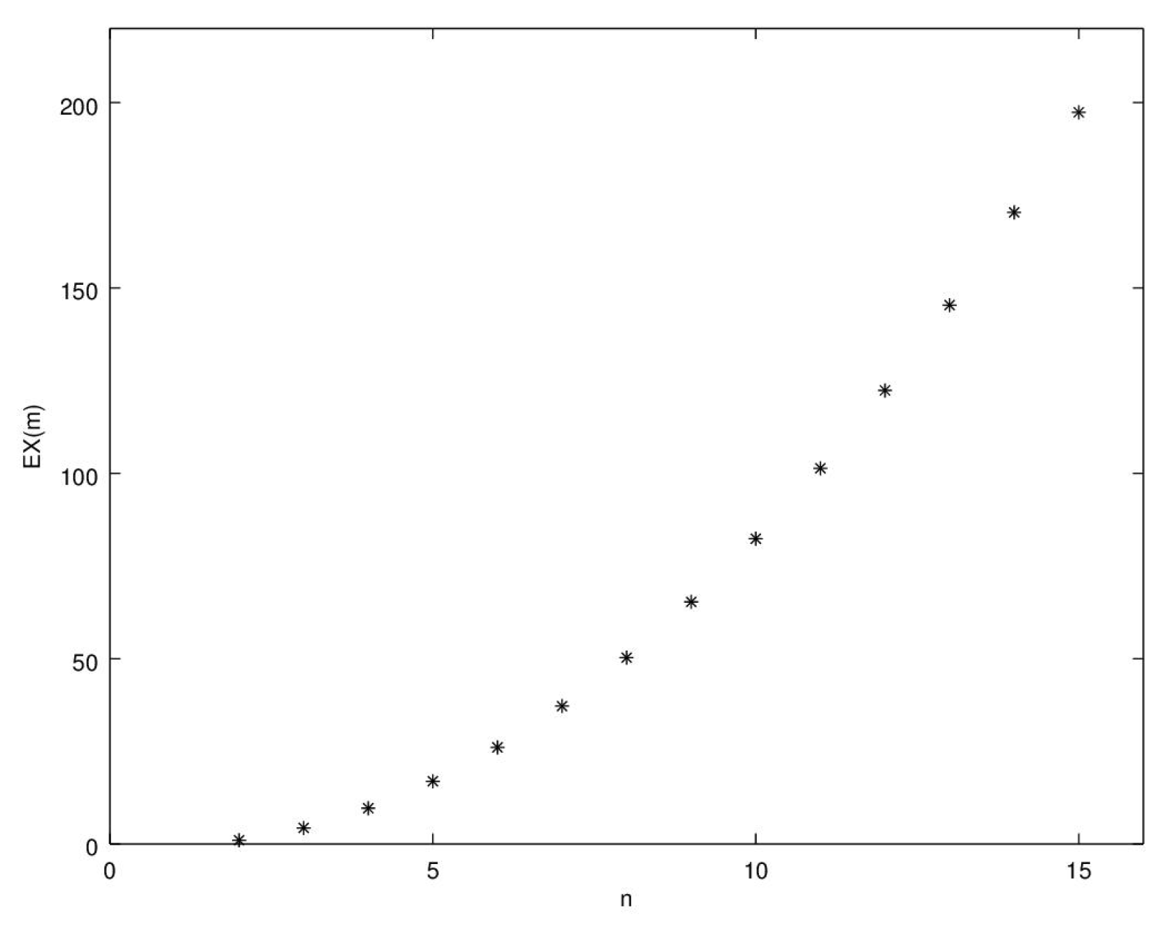
Example 4.
Given a frame of discernment X with cardinality n and a BPA m such that , for , we have
which are increasing with . We plot the values of the Deng extropy for in Figure 1. Deng entropy is not plotted because it is trivial.
Example 5.
Given a frame of discernment and a BPA m such that , , m(A) = 0.8, . When A changes, the following values for the Deng extropy and entropy in Table 1 are obtained:
As it was pointed out before, the results show that the extropy of m decreases monotonously with the rise of the size of subset A, while the entropy increases.
3. The Maximum Deng Extropy
Kang and Deng [26] studied the problem of the maximum Deng entropy. They find out that the maximum Deng entropy on a frame of discernment X with cardinality is attained if and only if the BPA m is defined as
where , , are all non-empty elements of . Hence, the value of the maximum Deng entropy is given by
In this section, we provide conditions to obtain the maximum Deng extropy for a fixed number of focal elements and with a fixed value for .
Theorem 1.
Let m be a BPA for a frame of discernment X. The maximum Deng extropy for fixed values of and N number of focal elements different from X, , is attained if and only if
In this case, the value of the maximum Deng extropy is
Proof.
Suppose . We will prove that in this case the maximum Deng extropy is
and that it is attained if and only if the BPA is defined by
We have to maximize
subject to the condition
Then, the Lagrange function can be defined as
Thus the gradient can be computed, and for we have
where does not depend on . By vanishing all the partial derivatives, we obtain
where K is a constant. It follows
By summing over , we get
and then
4. Application to Pattern Recognition
In this section, we investigate an application of the Deng extropy in pattern recognition by using the dataset Iris given in [27]. This example was already studied in [28] to analyze the applications of another belief entropy defined in the Dempster–Shafer evidence theory. We compare a method proposed by Kang [29] with a method based on the use of Deng extropy. The Iris dataset is useful to introduce the application of the generation of BPAs based on the Deng extropy in the classification of the kind of flowers. The dataset is composed of 150 samples. For each one, we have the sepal length in cm (SL), the sepal width in cm (SW), the petal length in cm (PL), the petal width in cm (PW) and the class that is only one between Iris Setosa (Se), Iris Versicolour (Ve) and Iris Virginica (Vi). The samples are equally distributed for each class. We select 40 samples for each kind of Iris and then we use sample of max–min value to generate a model of interval numbers, as shown in Table 2. Each element of the dataset can be regarded as an unknown test sample. Suppose the selected sample data is [6.1, 3.0, 4.9, 1.8, Iris Virginica].
Four BPAs are generated with a method proposed by Kang et al. based on the similarity of interval numbers [29]. Given two intervals and their similarity is defined as
where is the coefficient of support (we choose ) and is the distance of intervals A and B defined in [30] as
In order to generate BPAs, the intervals given in Table 2 are used as interval A and as interval B we use singletons given by the selected sample. For each one of the four properties, we get seven values of similarity and then we get a BPA by normalizing them (see Table 3). Hence, we evaluate the Deng extropy of these BPAs, as shown in the bottom row of Table 3. We obtain a combined BPA by using the Dempster rule of Combination (6). The type of unknown sample is determined by combined BPA. From Equation (4), we get the maximum value of PPT. Hence, Kang’s method assigns to the sample the type Iris Versicolour and it does not make the right decision.
Next, we use the Deng extropies given in Table 3 to generate other BPAs. We refer to these extropies as . We use these values as significance of each sample property to evaluate the weight of each property. For the sample property sepal length we have
We divide each weight for the maximum of the weights and use these values as discounting coefficients to generate new BPAs, as shown in Equation (5), see Table 4. Again, a combined BPA is obtained by using the Dempster rule of combination. The type of unknown sample is determined by combined BPA. Hence, the method based on the Deng extropy can make the right recognition.
We tested all 150 samples and we get that the global recognition rate of Kang’s method is 93.33% whereas the global recognition of the method based on the Deng extropy is 94%. The results are shown in Table 5.
5. Conclusions
In this paper, the Deng extropy has been defined as the dual measure of Deng entropy. Its relation with the analogous entropy has been analyzed and these measures have been compared in order to decide in which cases the first is better than the other one. Moreover, some examples are proposed. The behaviour of Deng extropy has been studied under changes of focal elements. We have given a characterization result for the maximum Deng extropy and, finally, a numerical example is discussed in order to highlight the relevance of this dual measure in pattern recognition.
Author Contributions
These authors contributed equally to this work. All authors have read and agreed to the published version of the manuscript.
Funding
This research received no external funding.
Acknowledgments
Francesco Buono and Maria Longobardi are partially supported by the GNAMPA research group of INdAM (Istituto Nazionale di Alta Matematica) and MIUR-PRIN 2017, Project “Stochastic Models for Complex Systems” (No. 2017 JFFHSH).
Conflicts of Interest
The authors declare no conflict of interest.
Abbreviations
The following abbreviations are used in this manuscript:
| BPA | Basic probability assignment |
| PPT | Pignistic probability transformation |
| SL | Sepal length in cm |
| SW | Sepal width in cm |
| PL | Petal length in cm |
| PW | Petal width in cm |
| Se | Iris Setosa |
| Ve | Iris Versicolour |
| Vi | Iris Virginica |
References
- Shannon, C.E. A mathematical theory of communication. Bell Labs. Tech. J. 1948, 27, 379–423. [Google Scholar] [CrossRef] [Green Version]
- Lad, F.; Sanfilippo, G.; Agrò, G. Extropy: Complementary dual of entropy. Stat. Sci. 2015, 30, 40–58. [Google Scholar] [CrossRef]
- Dempster, A.P. Upper and lower probabilities induced by a multivalued mapping. Ann. Math. Stat. 1967, 38, 325–339. [Google Scholar] [CrossRef]
- Shafer, G. A Mathematical Theory of Evidence; Princeton University Press: Princeton, NJ, USA, 1976. [Google Scholar]
- Deng, Y. Deng entropy. Chaos Solitons Fractals 2016, 91, 549–553. [Google Scholar] [CrossRef]
- Fu, C.; Yang, J.B.; Yang, S.L. A group evidential reasoning approach based on expert reliability. Eur. J. Oper. Res. 2015, 246, 886–893. [Google Scholar] [CrossRef]
- Yang, J.B.; Xu, D.L. Evidential reasoning rule for evidence combination. Artif. Intell. 2013, 205, 1–29. [Google Scholar] [CrossRef]
- Kabir, G.; Tesfamariam, S.; Francisque, A.; Sadiq, R. Evaluating risk of water mains failure using a Bayesian belief network model. Eur. J. Oper. Res. 2015, 240, 220–234. [Google Scholar] [CrossRef]
- Liu, H.C.; You, J.X.; Fan, X.J.; Lin, Q.L. Failure mode and effects analysis using D numbers and grey relational projection method. Expert Syst. Appl. 2014, 41, 4670–4679. [Google Scholar] [CrossRef]
- Han, Y.; Deng, Y. An enhanced fuzzy evidential DEMATEL method with its application to identify critical success factors. Soft Comput. 2018, 22, 5073–5090. [Google Scholar] [CrossRef]
- Liu, Z.; Pan, Q.; Dezert, J.; Han, J.W.; He, Y. Classifier fusion with contextual reliability evaluation. IEEE Trans. Cybern. 2018, 48, 1605–1618. [Google Scholar] [CrossRef]
- Smets, P. Data fusion in the transferable belief model. In Proceedings of the Third International Conference on Information Fusion, Paris, France, 10–13 July 2000; Volume 1, pp. PS21–PS33. [Google Scholar]
- Balakrishnan, N.; Buono, F.; Longobardi, M. On weighted extropies. Comm. Stat. Theory Methods. (under review).
- Calì, C.; Longobardi, M.; Ahmadi, J. Some properties of cumulative Tsallis entropy. Physica A 2017, 486, 1012–1021. [Google Scholar] [CrossRef] [Green Version]
- Calì, C.; Longobardi, M.; Navarro, J. Properties for generalized cumulative past measures of information. Probab. Eng. Inform. Sci. 2020, 34, 92–111. [Google Scholar] [CrossRef]
- Calì, C.; Longobardi, M.; Psarrakos, G. A family of weighted distributions based on the mean inactivity time and cumulative past entropies. Ricerche Mat. 2019, 1–15. [Google Scholar] [CrossRef]
- Di Crescenzo, A.; Longobardi, M. On cumulative entropies. J. Stat. Plann. Inference 2009, 139, 4072–4087. [Google Scholar] [CrossRef]
- Kamari, O.; Buono, F. On extropy of past lifetime distribution. Ricerche Mat. 2020, in press. [Google Scholar] [CrossRef]
- Longobardi, M. Cumulative measures of information and stochastic orders. Ricerche Mat. 2014, 63, 209–223. [Google Scholar] [CrossRef] [Green Version]
- Abellan, J. Analyzing properties of Deng entropy in the theory of evidence. Chaos Solitons Fractals 2017, 95, 195–199. [Google Scholar] [CrossRef]
- Tang, Y.; Fang, X.; Zhou, D.; Lv, X. Weighted Deng entropy and its application in uncertainty measure. In Proceedings of the 20th International Conference on Information Fusion (Fusion), Xi’an, China, 10–13 July 2017; pp. 1–5. [Google Scholar]
- Wang, D.; Gao, J.; Wei, D. A New Belief Entropy Based on Deng Entropy. Entropy 2019, 21, 987. [Google Scholar] [CrossRef] [Green Version]
- Hohle, U. Entropy with respect to plausibility measures. In Proceedings of the 12th IEEE International Symposium on Multiple-Valued Logic, Paris, France, 25–27 May 1982; pp. 167–169. [Google Scholar]
- Yager, R.R. Entropy and specificity in a mathematical theory of evidence. Int. J. Gen. Syst. 1983, 9, 249–260. [Google Scholar] [CrossRef]
- Klir, G.J.; Ramer, A. Uncertainty in the Dempster-Shafer theory: A critical re-examination. Int. J. Gen. Syst. 1990, 18, 155–166. [Google Scholar] [CrossRef]
- Kang, B.; Deng, Y. The Maximum Deng Entropy. IEEE Access 2019, 7, 120758–120765. [Google Scholar] [CrossRef]
- Dheeru, D.; Karra Taniskidou, E. UCI Machine Learning Repository. 2017. Available online: http://archive.ics.uci.edu/ml (accessed on 20 May 2020).
- Cui, H.; Liu, Q.; Zhang, J.; Kang, B. An Improved Deng Entropy and Its Application in Pattern Recognition. IEEE Access 2019, 7, 18284–18292. [Google Scholar] [CrossRef]
- Kang, B.Y.; Li, Y.; Deng, Y.; Zhang, Y.J.; Deng, X.Y. Determination of basic probability assignment based on interval numbers and its application. Acta Electron. Sin. 2012, 40, 1092–1096. [Google Scholar]
- Tran, L.; Duckstein, L. Comparison of fuzzy numbers using a fuzzy distance measure. Fuzzy Sets Syst. 2002, 130, 331–341. [Google Scholar] [CrossRef]
Figure 1.
in function of n with basic probability assignment (BPA) defined in Example 4.


Table 1.
The value of the Deng extropy and the Deng entropy when A changes.
| A | Deng Extropy | Deng Entropy |
|---|---|---|
| 28.104 | 2.6623 | |
| 27.904 | 3.9303 | |
| 27.704 | 4.9082 | |
| 27.504 | 5.7878 | |
| 27.304 | 6.6256 | |
| 27.104 | 7.4441 | |
| 26.903 | 8.2532 | |
| 26.702 | 9.0578 | |
| 26.500 | 9.8600 | |
| 26.295 | 10.661 | |
| 26.086 | 11.462 | |
| 25.866 | 12.262 | |
| 25.621 | 13.062 | |
| 25.304 | 13.862 |
Table 2.
The interval numbers of the statistical model.
| Item | SL | SW | PL | PW |
|---|---|---|---|---|
| [4.4,5.8] | [2.3,4.4] | [1.0,1.9] | [0.1,0.6] | |
| [4.9,7.0] | [2.0,3.4] | [3.0,5.1] | [1.0,1.7] | |
| [4.9,7.9] | [2.2,3.8] | [4.5,6.9] | [1.4,2.5] | |
| [4.9,5.8] | [2.3,3.4] | – | – | |
| [4.9,5.8] | [2.3,3.8] | – | – | |
| [4.9,7.0] | [2.2,3.4] | [4.5,5.1] | [1.4,1.7] | |
| [4.9,5.8] | [2.3,3.4] | – | – |
Table 3.
BPAs based on Kang’s method, Deng extropy and final fusion result.
| Item | SL | SW | PL | PW | Combined BPA |
|---|---|---|---|---|---|
| 0.1098 | 0.1018 | 0.0625 | 0.1004 | 0.0059 | |
| 0.1703 | 0.1303 | 0.1839 | 0.2399 | 0.4664 | |
| 0.1257 | 0.1385 | 0.1819 | 0.3017 | 0.4656 | |
| 0.1413 | 0.1663 | 0.0000 | 0.0000 | 0.0000 | |
| 0.1413 | 0.1441 | 0.0000 | 0.0000 | 0.0000 | |
| 0.1703 | 0.1527 | 0.5719 | 0.3580 | 0.0620 | |
| 0.1413 | 0.1663 | 0.0000 | 0.0000 | 0.0000 | |
| Deng extropy | 5.2548 | 5.2806 | 5.1636 | 4.9477 |
Table 4.
The modified BPAs based on the Deng extropy and final fusion result.
| Item | SL | SW | PL | PW | Combined BPA |
|---|---|---|---|---|---|
| 0.0808 | 0.0730 | 0.0504 | 0.1004 | 0.0224 | |
| 0.1252 | 0.0934 | 0.1482 | 0.2399 | 0.4406 | |
| 0.0925 | 0.0993 | 0.1465 | 0.3017 | 0.4451 | |
| 0.1039 | 0.1192 | 0.0000 | 0.0000 | 0.0000 | |
| 0.1039 | 0.1033 | 0.0000 | 0.0000 | 0.0000 | |
| 0.1252 | 0.1095 | 0.4608 | 0.3580 | 0.0919 | |
| 0.3684 | 0.4023 | 0.1942 | 0.0000 | 0.0000 |
Table 5.
The recognition rate.
| Item | Setosa | Versicolor | Virginica | Global |
|---|---|---|---|---|
| Kang’s method | 100% | 96% | 84% | 93.33% |
| Method based on Deng extropy | 100% | 96% | 86% | 94% |
© 2020 by the authors. Licensee MDPI, Basel, Switzerland. This article is an open access article distributed under the terms and conditions of the Creative Commons Attribution (CC BY) license (http://creativecommons.org/licenses/by/4.0/).
Share and Cite
MDPI and ACS Style
Buono, F.; Longobardi, M. A Dual Measure of Uncertainty: The Deng Extropy. Entropy 2020, 22, 582. https://0-doi-org.brum.beds.ac.uk/10.3390/e22050582
AMA Style
Buono F, Longobardi M. A Dual Measure of Uncertainty: The Deng Extropy. Entropy. 2020; 22(5):582. https://0-doi-org.brum.beds.ac.uk/10.3390/e22050582
Chicago/Turabian StyleBuono, Francesco, and Maria Longobardi. 2020. "A Dual Measure of Uncertainty: The Deng Extropy" Entropy 22, no. 5: 582. https://0-doi-org.brum.beds.ac.uk/10.3390/e22050582
Note that from the first issue of 2016, this journal uses article numbers instead of page numbers. See further details here.