Training Multilayer Perceptron with Genetic Algorithms and Particle Swarm Optimization for Modeling Stock Price Index Prediction


Abstract
:1. Introduction
2. Literature Review
Technical Indicators
3. Materials and Methods
3.1. Data
3.2. Methods
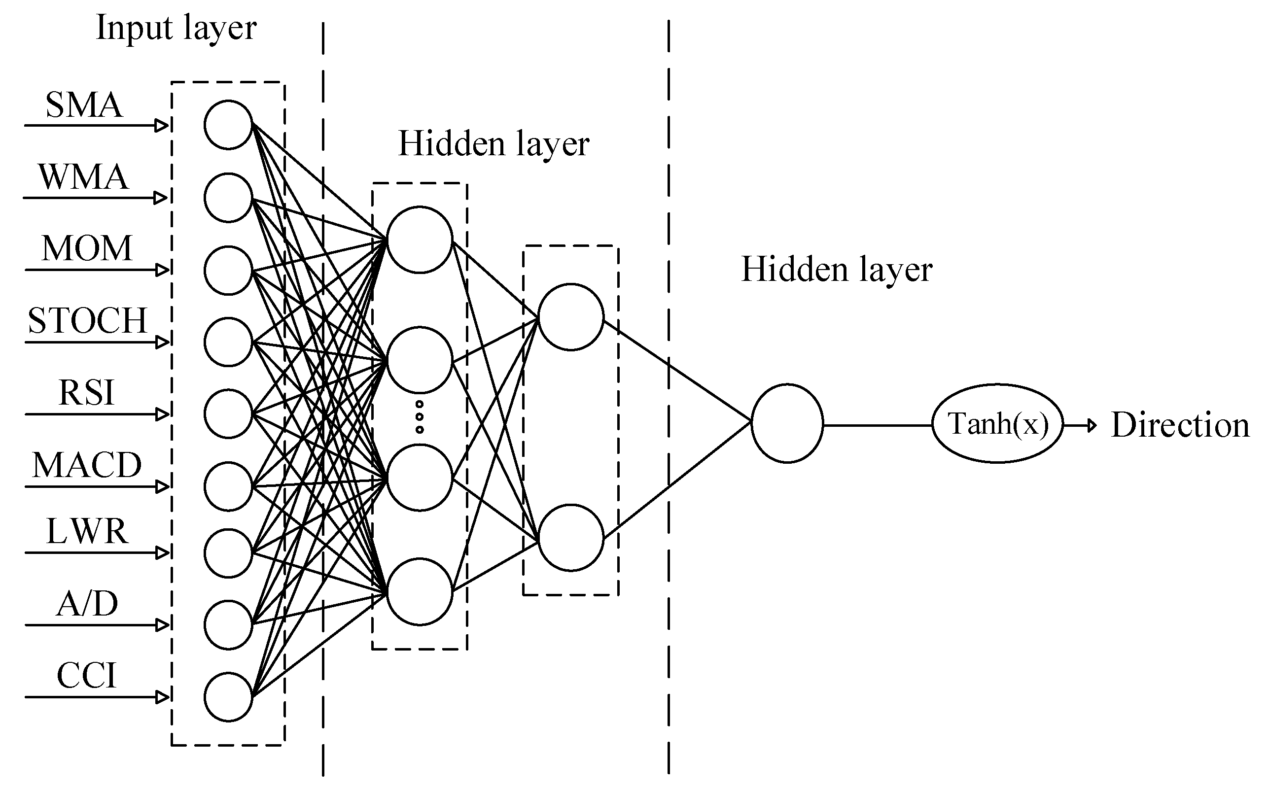
3.2.1. Multilayer Perceptron (MLP)
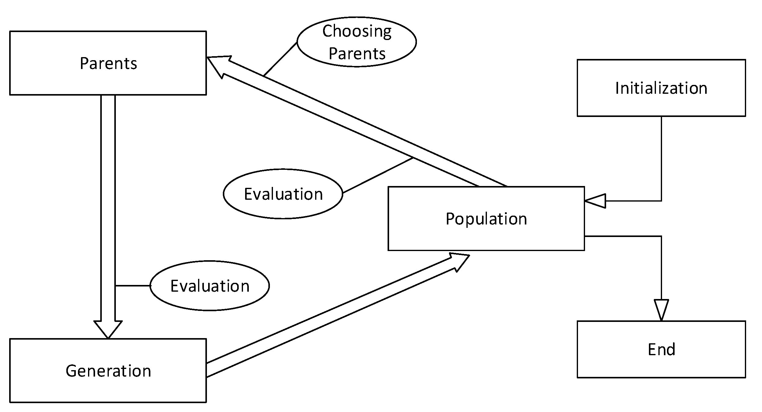
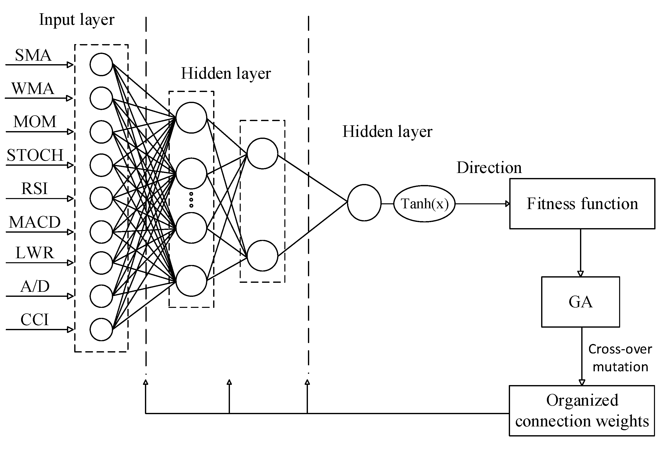
3.2.2. Genetic Algorithm (GA)
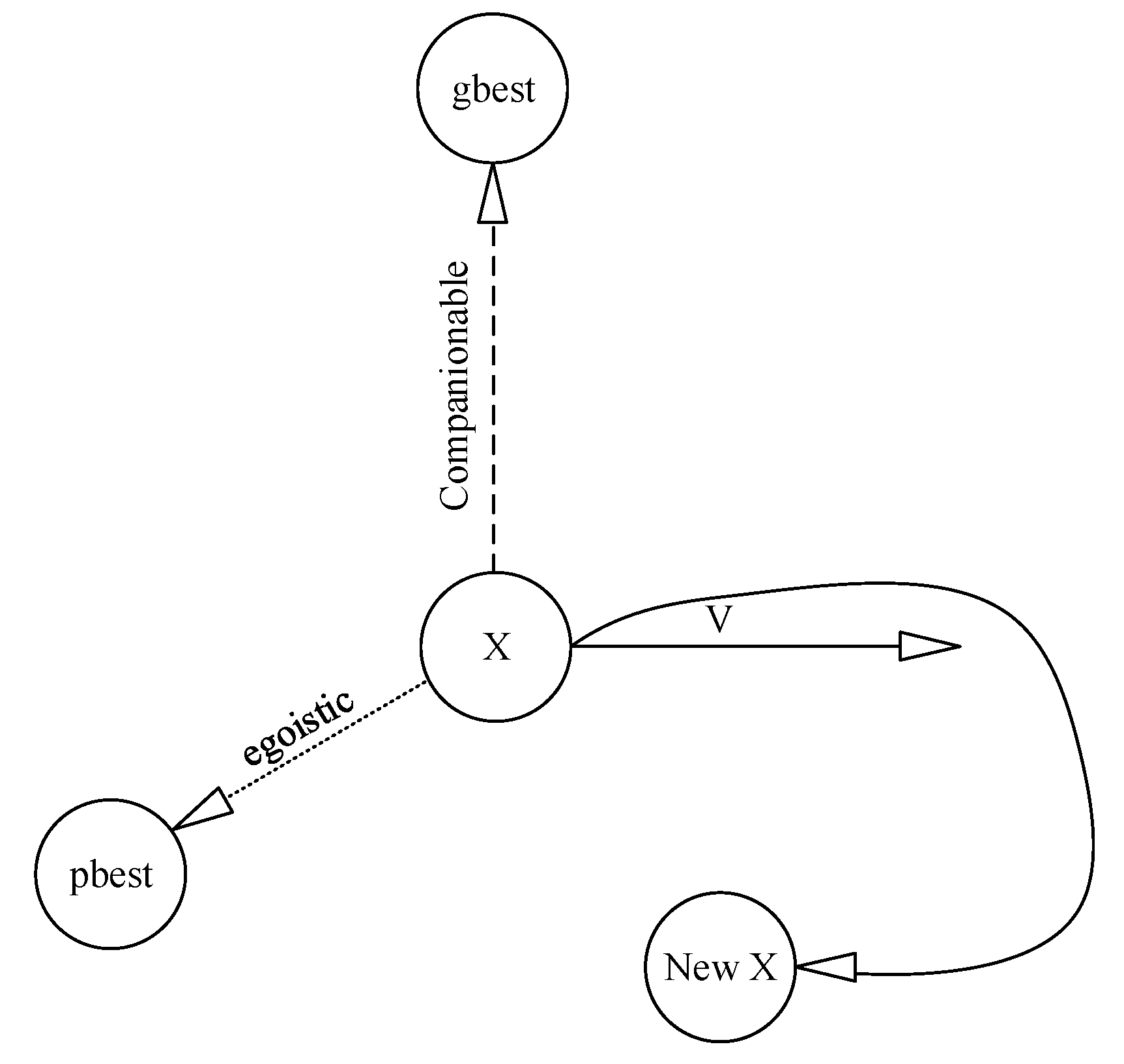
3.2.3. Particle Swarm Optimization (PSO)
- A certain number of repetitions,
- Achieve a decent threshold,
- A number of repetitions that do not change the competence (for example, if after 10 repetitions the competency was constant and did not improve),
- The last way is based on the aggregation density around the optimal point.
3.2.4. Training Phase
3.2.5. Evaluation Metrics
4. Results
Testing Results
5. Conclusions
Author Contributions
Funding
Acknowledgments
Conflicts of Interest
Abbreviations
| MLP | Multilayer perceptron | TEPIX | Tehran stock exchange price index |
| MV | Moving variance | LDA | linear discriminant analysis |
| GA | Genetic algorithms | BPNN | Back propagation neural network |
| RMSE | Root mean square error | BSE-SENSEX | Bombay Stock Exchange |
| ANN | Artificial neural network | TAPI 10 | 10-day total amount weight stock price index |
| MOM | momentum | ICA | Independent Component Analysis |
| SVM | Support vector machine | TAIEX | Taiwan Stock Exchange Capitalization Weighted Stock Index |
| ROC | rate of change | KOSPI | Korea Composite Stock Price Index |
| BIST 100 | Borsa Istanbul 100 index | MAPE | Mean Absolute Percentage Error |
| %D | stochastic D | CSI 300 | Capitalization-weighted SM index |
| CROBEX | Zagreb stock index | CNX Nifty | Standard & Poor’s CNX Nifty stock index |
| DAX-30 | German DAX-30 | DJIA | Dow Jones Industrial Average |
| HIS | Hang Seng Index | FTSE | Financial Times Stock Exchange |
| k-NN | k-nearest neighbor | QDA | quadratic discriminant analysis |
| S&P 500 | Standard & Poor’s 500 | GMM | Gaussian mixture model |
| RBF | Radial basis function | RKELM | Robust kernel extreme learning machine |
| SMA | simple moving average | KLCI | Kuala Lumpur Composite Index |
| RSI | relative strength index | BOVESPA | Bolsa de Valores de São Paulo |
| %K | stochastic K | PNN | Probabilistic neural network |
| %R | Larry William’s R% | A/D | Accumulation/Distribution |
| OSCP | price oscillator | CCI | Commodity Channel Index |
| SO | Stochastic oscillator | MSO | Moving stochastic oscillator |
| SSO | Slow stochastic oscillator | PSO | Particle swarm optimization |
| MVR | Moving variance ratio | EMA | Exponential moving average |
| LRL | Linear regression line | MACD | Moving average convergence and divergence |
| NB | Naive Bayes | SM | Stock market |
| RS | Rough sets | DWT | Discrete wavelet transform |
| IBEX-35 | Spanish SM | ARIMA | Autoregressive integrated moving average |
References
- Adebiyi, A.A.; Ayo, C.K.; Adebiyi, M.O.; Otokiti, S.O. Stock price prediction using neural network with hybridized market indicators. J. Emerg. Trends Comput. Inf. Sci. 2012, 3, 1–9. [Google Scholar]
- Hafezi, R.; Shahrabi, J.; Hadavandi, E. A bat-neural network multi-agent system (BNNMAS) for stock price prediction: Case study of DAX stock price. Appl. Soft Comput. 2015, 29, 196–210. [Google Scholar] [CrossRef]
- Liu, G.; Wang, X. A new metric for individual stock trend prediction. Eng. Appl. Artif. Intell. 2019, 82, 1–12. [Google Scholar] [CrossRef]
- Rahman, A.; Saadi, S. Random walk and breaking trend in financial series: An econometric critique of unit root tests. Rev. Financ. Econ. 2008, 17, 204–212. [Google Scholar] [CrossRef]
- Lo, A.W.; MacKinlay, A.C. Stock market prices do not follow random walks: Evidence from a simple specification test. Rev. Financ. Stud. 1988, 1, 41–66. [Google Scholar] [CrossRef]
- Vejendla, A.; Enke, D. Performance evaluation of neural networks and GARCH models for forecasting volatility and option strike prices in a bull call spread strategy. J. Econ. Policy Res. 2013, 8, 1. [Google Scholar]
- Chiang, W.-C.; Enke, D.; Wu, T.; Wang, R. An adaptive stock index trading decision support system. J. Econ. Policy Res. 2016, 59, 195–207. [Google Scholar] [CrossRef]
- Hadavandi, E.; Shavandi, H.; Ghanbari, A. Integration of genetic fuzzy systems and artificial neural networks for stock price forecasting. Knowl. Based Syst. 2010, 23, 800–808. [Google Scholar] [CrossRef]
- Enke, D.; Mehdiyev, N. Stock market prediction using a combination of stepwise regression analysis, differential evolution-based fuzzy clustering, and a fuzzy inference neural network. Intell. Autom. Soft Comput. 2013, 19, 636–648. [Google Scholar] [CrossRef]
- Qiu, M.; Song, Y.; Akagi, F. Application of artificial neural network for the prediction of stock market returns: The case of the Japanese stock market. Chaos Solitons Fractals 2016, 85, 1–7. [Google Scholar] [CrossRef]
- Gorgulho, A.; Neves, R.; Horta, N. Applying a GA kernel on optimizing technical analysis rules for stock picking and portfolio composition. Expert Syst. Appl. 2011, 38, 14072–14085. [Google Scholar] [CrossRef]
- Lin, X.; Yang, Z.; Song, Y. Intelligent stock trading system based on improved technical analysis and Echo State Network. Expert Syst. Appl. 2011, 38, 11347–11354. [Google Scholar] [CrossRef]
- Cervelló-Royo, R.; Guijarro, F.; Michniuk, K. Stock market trading rule based on pattern recognition and technical analysis: Forecasting the DJIA index with intraday data. Expert Syst. Appl. 2015, 42, 5963–5975. [Google Scholar] [CrossRef]
- Chen, Y.-S.; Cheng, C.-H.; Tsai, W.-L. Modeling fitting-function-based fuzzy time series patterns for evolving stock index forecasting. Appl. Intell. 2014, 41, 327–347. [Google Scholar] [CrossRef]
- Yao, J.; Tan, C.L.; Poh, H.-L. Neural networks for technical analysis: A study on KLCI. Int. J. Theor. Appl. Financ. 1999, 2, 221–241. [Google Scholar] [CrossRef] [Green Version]
- Kim, K.-J. Financial time series forecasting using support vector machines. Neurocomputing 2003, 55, 307–319. [Google Scholar] [CrossRef]
- Nair, B.B.; Mohandas, V.; Sakthivel, N.R. A decision tree—Rough set hybrid system for stock market trend prediction. Int. J. Comput. Appl. 2010, 6, 1–6. [Google Scholar] [CrossRef]
- De Oliveira, F.A.; Nobre, C.N.; Zarate, L.E. Applying Artificial Neural Networks to prediction of stock price and improvement of the directional prediction index—Case study of PETR4, Petrobras, Brazil. Expert Syst. Appl. 2013, 40, 7596–7606. [Google Scholar] [CrossRef]
- Shakeri, B.; Zarandi, M.F.; Tarimoradi, M.; Turksan, I. Fuzzy clustering rule-based expert system for stock price movement prediction. In Proceedings of the 2015 Annual Conference of the North American Fuzzy Information Processing Society (NAFIPS), Redmond, WA, USA, 17–19 August 2015; pp. 1–6. [Google Scholar]
- Patel, J.; Shah, S.; Thakkar, P.; Kotecha, K. Predicting stock and stock price index movement using trend deterministic data preparation and machine learning techniques. Expert Syst. Appl. 2015, 42, 259–268. [Google Scholar] [CrossRef]
- Santoso, M.; Sutjiadi, R.; Lim, R. Indonesian Stock Prediction using Support Vector Machine (SVM). In MATEC Web of Conferences; EDP Sciences: Les Ulis, France, 2018; p. 01031. [Google Scholar]
- Chandar, S.K. Stock market prediction using subtractive clustering for a neuro fuzzy hybrid approach. Clust. Comput. 2019, 22, 13159–13166. [Google Scholar] [CrossRef]
- Cervelló-Royo, R.; Guijarro, F. Forecasting stock market trend: A comparison of machine learning algorithms. Financ. Mark. Valuat. 2020, 6, 37–49. [Google Scholar]
- Kara, Y.; Boyacioglu, M.A.; Baykan, Ö.K. Predicting direction of stock price index movement using artificial neural networks and support vector machines: The sample of the Istanbul Stock Exchange. Expert Syst. Appl. 2011, 38, 5311–5319. [Google Scholar] [CrossRef]
- Karymshakov, K.; Abdykaparov, Y. Forecasting stock index movement with artificial neural networks: The case of istanbul stock exchange. Trak. Univ. J. Soc. Sci. 2012, 14, 231–241. [Google Scholar]
- Lahmiri, S. Minute-ahead stock price forecasting based on singular spectrum analysis and support vector regression. Appl. Math. Comput. 2018, 320, 444–451. [Google Scholar] [CrossRef]
- Pulido, M.; Melin, P.; Castillo, O. Particle swarm optimization of ensemble neural networks with fuzzy aggregation for time series prediction of the Mexican Stock Exchange. Inf. Sci. 2014, 280, 188–204. [Google Scholar] [CrossRef]
- Lahmiri, S. Interest rate next-day variation prediction based on hybrid feedforward neural network, particle swarm optimization, and multiresolution techniques. Phys. A Stat. Mech. Appl. 2016, 444, 388–396. [Google Scholar] [CrossRef]
- Aldin, M.M.; Dehnavi, H.D.; Entezari, S. Evaluating the employment of technical indicators in predicting stock price index variations using artificial neural networks (case study: Tehran Stock Exchange). Int. J. Bus. Manag. 2012, 7, 25. [Google Scholar]
- Gurjar, M.; Naik, P.; Mujumdar, G.; Vaidya, T. Stock market prediction using ANN. Int. Res. J. Eng. Technol. (IRJET) 2018, 5, 2758–2761. [Google Scholar]
- Yu, L.; Wang, S.; Lai, K.K. Mining stock market tendency using GA-based support vector machines. In Proceedings of the First International Workshop on Internet and Network Economics, Hong Kong, China, 15–17 December 2005; pp. 336–345. [Google Scholar]
- Lu, C.-J. Integrating independent component analysis-based denoising scheme with neural network for stock price prediction. Expert Syst. Appl. 2010, 37, 7056–7064. [Google Scholar] [CrossRef]
- Dash, R.; Dash, P. Efficient stock price prediction using a self evolving recurrent neuro-fuzzy inference system optimized through a modified differential harmony search technique. Expert Syst. Appl. 2016, 52, 75–90. [Google Scholar] [CrossRef]
- Lahmiri, S. A comparison of PNN and SVM for stock market trend prediction using economic and technical information. Int. J. Comput. Appl. 2011, 29, 24–30. [Google Scholar]
- Dastgir, M.; Enghiad, M.H. Short-term prediction of Tehran Stock Exchange Price Index (TEPIX): Using artificial neural network (ANN). J. Secur. Exch. 2012, 4, 237–261. [Google Scholar]
- Dunis, C.L.; Rosillo, R.; de la Fuente, D.; Pino, R. Applications. Forecasting IBEX-35 moves using support vector machines. Neural Comput. Appl. 2013, 23, 229–236. [Google Scholar] [CrossRef]
- Lahmiri, S.; Boukadoum, M.; Chartier, S. Information fusion and S&P500 trend prediction. In Proceedings of the 2013 ACS International Conference on Computer Systems and Applications (AICCSA), Ifrane, Morocco, 27–30 May 2013; pp. 1–7. [Google Scholar]
- Wang, S.; Shang, W. Forecasting direction of China security index 300 movement with least squares support vector machine. Procedia Comput. Sci. 2014, 31, 869–874. [Google Scholar] [CrossRef] [Green Version]
- Anbalagan, T.; Maheswari, S.U. Classification and prediction of stock market index based on fuzzy metagraph. Procedia Comput. Sci. 2015, 47, 214–221. [Google Scholar] [CrossRef] [Green Version]
- Ballings, M.; Van den Poel, D.; Hespeels, N.; Gryp, R. Evaluating multiple classifiers for stock price direction prediction. Expert Syst. Appl. 2015, 42, 7046–7056. [Google Scholar] [CrossRef]
- Anish, C.; Majhi, B. Hybrid nonlinear adaptive scheme for stock market prediction using feedback FLANN and factor analysis. J. Korean Stat. Soc. 2016, 45, 64–76. [Google Scholar] [CrossRef]
- Jabbarzadeh, A.; Shavvalpour, S.; Khanjarpanah, H.; Dourvash, D. A multiple-criteria approach for forecasting stock price direction: Nonlinear probability models with application in S&P 500 Index. Int. J. Appl. Eng. Res. 2016, 11, 3870–3878. [Google Scholar]
- Jiao, Y.; Jakubowicz, J. Predicting stock movement direction with machine learning: An extensive study on S&P 500 stocks. In Proceedings of the 2017 IEEE International Conference on Big Data (Big Data), Boston, MA, USA, 11–14 December 2017; pp. 4705–4713. [Google Scholar]
- Garcia, F.; Guijarro, F.; Oliver, J.; Tamošiūnienė, R. Hybrid fuzzy neural network to predict price direction in the German DAX-30 index. Technol. Econ. Dev. Econ. 2018, 24, 2161–2178. [Google Scholar] [CrossRef]
- Nadh, V.L.; Prasad, G.S. Stock market prediction based on machine learning approaches. In Computational Intelligence and Big Data Analytics; Springer: Berlin/Heidelberg, Germany, 2019; pp. 75–79. [Google Scholar]
- Manojlović, T.; Štajduhar, I. Predicting stock market trends using random forests: A sample of the Zagreb stock exchange. In Proceedings of the 2015 38th International Convention on Information and Communication Technology, Electronics and Microelectronics (MIPRO), Opatija, Croatia, 25–29 May 2015; pp. 1189–1193. [Google Scholar]
- Malagrino, L.S.; Roman, N.T.; Monteiro, A.M. Forecasting stock market index daily direction: A Bayesian Network approach. Expert Syst. Appl. 2018, 105, 11–22. [Google Scholar] [CrossRef]
- Dash, R.; Samal, S.; Rautray, R.; Dash, R. A TOPSIS approach of ranking classifiers for stock index price movement prediction. In Soft Computing in Data Analytics; Springer: Berlin/Heidelberg, Germany, 2019; pp. 665–674. [Google Scholar]
- Bisoi, R.; Dash, P.; Parida, A. Hybrid Variational Mode Decomposition and evolutionary robust kernel extreme learning machine for stock price and movement prediction on daily basis. Appl. Soft Comput. 2019, 74, 652–678. [Google Scholar] [CrossRef]
- Ecer, F. Artificial Neural Networks in Predicting Financial Performance: An Application for Turkey’s Top 500 Companies. Econ. Comput. Econ. Cybern. Studies Res. 2013, 47, 103–114. [Google Scholar]
- Ardabili, S.F.; Mahmoudi, A.; Gundoshmian, T.M. Modeling and simulation controlling system of HVAC using fuzzy and predictive (radial basis function, RBF) controllers. J. Build. Eng. 2016, 6, 301–308. [Google Scholar] [CrossRef]
- Ecer, F. Comparing the bank failure prediction performance of neural networks and support vector machines: The Turkish case. Econ. Res. 2013, 26, 81–98. [Google Scholar] [CrossRef] [Green Version]
- Gundoshmian, T.M.; Ardabili, S.; Mosavi, A.; Varkonyi-Koczy, A.R. Prediction of combine harvester performance using hybrid machine learning modeling and response surface methodology. In Proceedings of the International Conference on Global Research and Education, Balatonfüred, Hungary, 4–7 September 2019. [Google Scholar]
- Ardabili, S.F. Simulation and Comparison of Control System in Mushroom Growing Rooms Environment. Master’s Thesis, University of Tabriz, Tabriz, Iran, 2014. [Google Scholar]
- Lee, T.K.; Cho, J.H.; Kwon, D.S.; Sohn, S.Y. Global stock market investment strategies based on financial network indicators using machine learning techniques. Expert Syst. Appl. 2019, 117, 228–242. [Google Scholar] [CrossRef]
- Zhong, X.; Enke, D. Predicting the daily return direction of the stock market using hybrid machine learning algorithms. Financ. Innov. 2019, 1, 14–24. [Google Scholar] [CrossRef]
- Harik, G.R.; Lobo, F.G.; Goldberg, D.E. The compact genetic algorithm. IEEE Trans. Evol. Comput. 1999, 3, 287–297. [Google Scholar] [CrossRef] [Green Version]
- Khan, W. Predicting stock market trends using machine learning algorithms via public sentiment and political situation analysis. Soft Comput. 2019, 12, 1–25. [Google Scholar] [CrossRef]
- Mühlenbein, H.; Schomisch, M.; Born, J. The parallel genetic algorithm as function optimizer. Parallel Comput. 1991, 17, 619–632. [Google Scholar] [CrossRef]
- Kampouropoulos, K.; Andrade, F.; Sala, E.; Espinosa, A.G.; Romeral, L. Multiobjective optimization of multi-carrier energy system using a combination of ANFIS and genetic algorithms. IEEE Trans. Smart Grid 2018, 9, 2276–2283. [Google Scholar] [CrossRef] [Green Version]
- Sahay, R.R.; Srivastava, A. Predicting monsoon floods in rivers embedding wavelet transform, genetic algorithm and neural network. Water Resour. Manag. 2014, 28, 301–317. [Google Scholar] [CrossRef]
- Wang, J.; Wan, W. Optimization of fermentative hydrogen production process using genetic algorithm based on neural network and response surface methodology. Int. J. Hydrog. Energy 2009, 34, 255–261. [Google Scholar] [CrossRef]
- Maertens, K.; De Baerdemaeker, J.; Babuška, R. Genetic polynomial regression as input selection algorithm for non-linear identification. Soft Comput. 2006, 10, 785–795. [Google Scholar] [CrossRef]
- Pandey, P.M.; Thrimurthulu, K.; Reddy, N.V. Optimal part deposition orientation in FDM by using a multicriteria genetic algorithm. Int. J. Prod. Res. 2004, 42, 4069–4089. [Google Scholar] [CrossRef]
- Horn, J.; Nafpliotis, N.; Goldberg, D.E. A niched Pareto genetic algorithm for multiobjective optimization. In Proceedings of the First IEEE Conference on Evolutionary Computation (IEEE World Congress on Computational Intelligence), Orlando, FL, USA, 27–29 June 1994; pp. 82–87. [Google Scholar]
- Mansoor, A.-K.Z.; Salih, T.A.; Hazim, M.Y. Self-tuning PID Controller using Genetic Algorithm. Iraqi J. Stat. Sci. 2011, 11, 369–385. [Google Scholar]
- Song, S.; Singh, V.P. Frequency analysis of droughts using the Plackett copula and parameter estimation by genetic algorithm. Stoch. Environ. Res. Risk Assess. 2010, 24, 783–805. [Google Scholar] [CrossRef]
- Abdullah, S.S.; Malek, M.; Abdullah, N.S.; Mustapha, A. Feedforward backpropagation, genetic algorithm approaches for predicting reference evapotranspiration. Sains Malays. 2015, 44, 1053–1059. [Google Scholar] [CrossRef]
- Poli, R.; Kennedy, J.; Blackwell, T. Particle swarm optimization. Swarm Intell. 2007, 1, 33–57. [Google Scholar] [CrossRef]
- Sun, J.; Feng, B.; Xu, W. Particle swarm optimization with particles having quantum behavior. In Proceedings of the 2004 Congress on Evolutionary Computation (IEEE Cat. No. 04TH8753), Portland, OR, USA, 19–23 June 2004; pp. 325–331. [Google Scholar]
- Parsopoulos, K.E.; Vrahatis, M.N. Particle swarm optimization method in multiobjective problems. In Proceedings of the 2002 ACM symposium on Applied computing, New York, NY, USA, 22–27 March 2002; pp. 603–607. [Google Scholar]
- Kennedy, J.; Eberhart, R. Particle swarm optimization. In Proceedings of the ICNN’95-International Conference on Neural Networks, Perth, WA, Australia, 27 November–1 December 1995; pp. 1942–1948. [Google Scholar]
- Baltar, A.M.; Fontane, D.G. Use of multiobjective particle swarm optimization in water resources management. J. Water Resour. Plan. Manag. 2008, 134, 257–265. [Google Scholar] [CrossRef]
- Clerc, M. Particle Swarm Optimization; John Wiley & Sons: Hoboken, NJ, USA, 2010; Volume 93. [Google Scholar]
- Shi, Y. Particle swarm optimization: Developments, applications and resources. In Proceedings of the 2001 Congress on Evolutionary Computation (IEEE Cat. No. 01TH8546), Seoul, Korea, 27–30 May 2001; pp. 81–86. [Google Scholar]
- Shi, Y.; Eberhart, R.C. Parameter selection in particle swarm optimization. In Proceedings of the International Conference on Evolutionary Programming, San Diego, CA, USA, 25–27 March 1998; pp. 591–600. [Google Scholar]
- Allaoua, B.; Laoufi, A.; Gasbaoui, B.; Abderrahmani, A. Technologies. Neuro-fuzzy DC motor speed control using particle swarm optimization. Leonardo Electron. J. Pract. Technol. 2009, 15, 1–18. [Google Scholar]
- Gharghan, S.K.; Nordin, R.; Ismail, M.; Ali, J.A. Accurate wireless sensor localization technique based on hybrid PSO-ANN algorithm for indoor and outdoor track cycling. IEEE Sensors J. 2015, 16, 529–541. [Google Scholar] [CrossRef]
- Armaghani, D.J.; Raja, R.S.N.S.B.; Faizi, K.; Rashid, A.S.A. Developing a hybrid PSO–ANN model for estimating the ultimate bearing capacity of rock-socketed piles. Neural Comput. Appl. 2017, 28, 391–405. [Google Scholar] [CrossRef]
- Liou, S.-W.; Wang, C.-M.; Huang, Y.-F. Integrative Discovery of Multifaceted Sequence Patterns by Frame-Relayed Search and Hybrid PSO-ANN. J. UCS 2009, 15, 742–764. [Google Scholar]
- Pang, X.; Zhou, Y.; Wang, P.; Lin, W.; Chang, V. An innovative neural network approach for stock market prediction. J. Supercomput. 2020, 76, 2098–2118. [Google Scholar] [CrossRef]
- Mosavi, A.; Salimi, M.; Faizollahzadeh Ardabili, S.; Rabczuk, T.; Shamshirband, S.; Varkonyi-Koczy, A.R. State of the art of machine learning models in energy systems, a systematic review. Energies 2019, 12, 1301. [Google Scholar] [CrossRef] [Green Version]
- Liu, H.; Long, Z. An improved deep learning model for predicting stock market price time series. Digit. Signal Process. 2020, 7, 102741. [Google Scholar] [CrossRef]
- Nabipour, M.; Nayyeri, P.; Jabani, H.; Shahab, S.; Mosavi, A. Predicting Stock Market Trends Using Machine Learning and Deep Learning Algorithms Via Continuous and Binary Data: A Comparative Analysis. IEEE Access 2020, 8, 150199–150212. [Google Scholar] [CrossRef]
- Nabipour, M.; Nayyeri, P.; Jabani, H.; Mosavi, A.; Salwana, E. Deep learning for stock market prediction. Entropy 2020, 22, 840. [Google Scholar] [CrossRef]


| References | Method/s | Application/Data | Result |
|---|---|---|---|
| [15] | ANN, ARIMA | KLCI (1984–1991) | ANN outperformed ARIMA model. |
| [16] | SVM, BPNN | KOSPI (1989–1998) | SVM outperformed ANN. |
| [32] | ICA–BPNN, BPNN | TAIEX (2003–2006) | ICA–BPNN is superior. |
| [17] | ANN, NB, DT | BSE (2003–2010) | Hybrid RSs outperformed ANN. |
| [34] | PNN, SVM | S&P 500 (2000–2008) | PNN provided high accuracy. |
| [24] | ANN, SVM | BIST 100 (1997–2007) | 75% accuracy using ANN. |
| [29] | ANN | TEPIX (2002–2009) | ANN showed promising results. |
| [35] | ANN, GA | TEPIX (2000–2008) | ANN delivered next day estimates. |
| [25] | ANN | BIST 100 (2002–2007) | ANN achieved success with 82.7%. |
| [36] | SVM, ANN | IBEX-35 (1990–2010) | SVM outperformed ANN. |
| [37] | k-NN, PNN | S&P 500 (2003–2008) | k-NN outperformed PNN. |
| [18] | ANN | BOVESPA (2000–2011) | ANN suitable for direction estimation. |
| [38] | LSSVM, PNN, | CSI 300 (2005–2012) | LSSVM outperformed other models. |
| [39] | Random walk, ANN, SVM, fuzzy | BSE-SENSEX (2011–2012) | The fuzzy metagraph-based model has reached a classification rate of 75%. |
| [40] | ANN, RF, k-NN | Amadeus (2009–2010) | RF outperformed ANN. |
| [20] | NB, ANN, SVM | CNX Nifty (2003–2012) | NB outperformed other models. |
| [41] | DWT, ANN, SVM–MLP | DJIA-S&P500 (2000–2012) | SVM–MLP is superior. |
| [42] | Probit, Logit, Extreme Value | S&P 500 (2011–2015) | Extreme Value outperfomed Logit and Probit. |
| [7] | PSO–ANN | S&P 500, IXIC (2008–2010) | Acceptable prediction and robustness. |
| [43] | RF & ANN | S&P 500 (2009–2017) | RF outperformed ANN. |
| [44] | Hybrid fuzzy NN | DAX-30 (1999–2017) | minimum risky strategies. |
| [45] | GA, SVM, ANN | BM&FBOVESPA PETR4 (1999–2017) | SVM performed better than ANN. |
| Author/s | Method/s | Application | Result |
|---|---|---|---|
| [31] | GA–SVM, random walk, SVM, ARIMA, BPNN | S&P 500 (2000–2004) | GA–SVM has been shown to outperform other models. |
| [14] | Fuzzy sets, physical, support vector regression, partial least squares regression | TAIEX and HIS (1998–2006) | Their proposed models outperform the compared models according to the RMSE. |
| [46] | Random forest | CROBEX (2008–2013) | Random forests can be successfully preferred to estimate. |
| [19] | Fuzzy rule-based expert system | Apple company (2010–2014) | The fuzzy expert system has significant performance with minimal error. |
| [21] | GMM–SVM | Indonesia ASII.JK (2000–2017) | The GMM–SVM model has been found to be superior to other models. |
| [47] | Bayesian network | iBOVESPA (2005–2012) | Mean accuracy with the proposed model configuration was almost 71%. |
| [48] | TOPSIS, SVM, NB, Decision tree, kNN | BSE SENSEX, S&P500 (2015–2017) | While SVM model performs better in BSE SENSEX index, k-NN is superior to other models in S&P 500 index. |
| [22] | ANFIS | Apple stock data (2005–2015) | The proposed method outperformed the existing methods. |
| [49] | RKELM | BSE, HIS, FTSE (2010–2015) | They proved the superiority of the RKELM model over the ANN, naive Bayes and SVM. |
| [3] | Mean Profit Rate (MPR) | DJIA, S&P500, HSI, Nikkei 225, SSE (2007–2017) | MPR is an effective classifier. |
| Author/s | Technical Indicators |
|---|---|
| [15] | Simple moving average (SMA), stochastic K (%K), momentum (MOM), stochastic D (%D), relative strength index (RSI). |
| [16] | Slow D%, MOM, rate of change (ROC), K%, Larry William’s R% (%R), Accumulation/Distribution (A/D) oscillator, disparity5, RSI, disparity10, price oscillator (OSCP), D%, Commodity Channel Index (CCI). |
| [31] | OSCP, Stochastic oscillator (SO), Slow stochastic oscillator (SSO), CCI, ROC, MOM, SMA, Moving variance (MV), Moving variance ratio (MVR), Exponential moving average (EMA), Moving average convergence and divergence (MACD), A/D oscillator, Price (P), disparity5, disparity10, Moving stochastic oscillator (MSO), RSI, linear regression line (LRL). |
| [32] | The previous day’s cash market high, low, volume, 6-day RSI, today’s opening cash index, 10-day total amount weighted stock price index. |
| [17] | %K, Positive volume index, %R, negative volume index, %D, on balance volume, RSI, MACD, MOM, A/D oscillator, 25-day SMA. |
| [34] | SMA, OSCP, MOM, %D, ROC, disparity, %K. |
| [29] | MACD, SMA, %R, CCI, A/D oscillator, %D, weighted moving average (WMA), RSI, MOM, %K. |
| [24] | %D, %K, RSI, MOM, MACD, WMA, %R, A/D oscillator, SMA, CCI. |
| [35] | SMA, MACD, RSI, OSCP, MOM, volume. |
| [18] | MACD, RSI, %D, SMA, Bollinger band, MOM, %R. |
| [14] | SMA for 5 days, SMA for 10 days, bias to moving average (BIAS), RSI, psychological line (PSY), %R, MACD, MOM. |
| [38] | %K, %R, %D, CCI, A/D oscillator, MOM, MACD, RSI, SMA and WMA. |
| [39] | MA, exponential moving average (EMA), MACD, RSI. |
| [19] | High price, low price, volume, change of closed price, MACD, MA, BIAS, RSI, %R. |
| [20] | %D, RSI, WMA, MACD, CCI, A/D oscillator, %K, %R, SMA. |
| [46] | 5-day SMA, 5-day WMA, 10-day SMA, 10-day WMA, %K, %D, MACD, CCI, 5-day disparity, 10-day disparity, OSCP, ROC, MOM, RSI, 5-day standard deviation. |
| [41] | SMA, EMA, A/D oscillator, %K, RSI, OSCP, closing price, maximum price. |
| [42] | SMA, WMA, MOM, %K, %D, %R, RSI, MACD. |
| [7] | Change of price, change of volume, 5-day SMA, 10-day SMA, 30-day SMA, moving price level (30 days), moving price level (120 days), percentage price oscillator. |
| [21] | A/D oscillator, mean of rising days, CCI, SMA, MACD, MOM, on balance volume, ratio of rising days, RSI, %R. |
| [44] | Triangular moving average (TMA), RSI, SMA, EMA, modified moving averages (MMA), volatility ratio (VR), %R, true strength index (TSI), average true range (ATR). |
| [48] | SMA, %K, %D, %R, MACD, RSI. |
| [45] | SMA, WMA, MOM, RSI. |
| [22] | 1-week SMA, 2-week SMA, 14-day disparity, R%. |
| [3] | %D, %K, RSI, MOM, MACD, WMA, %R, A/D oscillator, SMA, CCI. |
| [49] | SMA, MACD, %K, %D, RSI, %R. |
| Technical Indicators | Abbreviation | Formulas |
|---|---|---|
| Simple n (10 here)-day Moving Average | SMA | |
| Simple n (10 here)-day Moving Average | WMA | |
| Momentum | MOM | |
| Stochastic D% | STOCH | |
| Relative Strength Index | RSI | |
| Moving Average Convergence Divergence | MACD | |
| Larry William’s R% | LWR | |
| Accumulation/Distribution Oscillator | A/D | |
| Commodity Channel Index | CCI |
| Input Neuron | 9 |
| Hidden layer | 2 |
| Hidden layer activation function | Logsig |
| Output layer activation function | Gaussian, Tanh (x) |
| Pop. type | Double vector |
| Pop. size | 50, 100 and 150 |
| Crossover function | Scattered |
| Crossover fraction | 0.8 |
| Selection function | Uniform |
| Migration interval | 10 |
| Migration fraction | 0.2 |
| Input Neuron | 9 |
| Hidden layer | 2 |
| Hidden layer activation function | logsig |
| Output layer activation function | Gaussian, Tanh (x) |
| Number of Max. Iteration | 500 |
| Pop. size | 50, 75, 100 and 125 |
| c1 | 2 |
| c2 | 2 |
| Model 1 | MLP (9-10-2-1) | Model 8 | MLP–GA (100) |
| Model 2 | MLP (9-12-2-1) | Model 9 | MLP–GA (150) |
| Model 3 | MLP (9-14-2-1) | Model 10 | MLP–PSO (50) |
| Model 4 | MLP (9-15-2-1) | Model 11 | MLP–PSO (75) |
| Model 5 | MLP (9-17-2-1) | Model 12 | MLP–PSO (100) |
| Model 6 | MLP (9-19-2-1) | Model 13 | MLP–PSO (125) |
| Model 7 | MLP–GA (50) |
| Accuracy and Performance Index | Description |
|---|---|
| Correlation coefficient = | N: Number of Data X: Target value Y: Output value. |
| RMSE = |
| Model | Correlation Coefficient | RMSE | MAPE (%) | Processing Time (s) | Model | Correlation Coefficient | RMSE | MAPE (%) | Processing Time (s) |
|---|---|---|---|---|---|---|---|---|---|
| Model 1 | 0.67 | 0.741035 | 32.02% | 3.82 | Model 8 | 0.694 | 0.718928 | 30.57% | 8.33 |
| Model 2 | 0.68 | 0.733079 | 31.55% | 4.11 | Model 9 | 0.70 | 0.713458 | 30.31% | 10.82 |
| Model 3 | 0.676 | 0.735209 | 31.52% | 4.97 | Model 10 | 0.692 | 0.721568 | 30.40% | 6.78 |
| Model 4 | 0.682 | 0.730448 | 30.88% | 5.11 | Model 11 | 0.689 | 0.724479 | 30.89% | 7.32 |
| Model 5 | 0.689 | 0.723326 | 30.84% | 5.22 | Model 12 | 0.693 | 0.720478 | 30.28% | 9.02 |
| Model 6 | 0.693 | 0.719818 | 30.59% | 5.30 | Model 13 | 0.704 | 0.708774 | 29.93% | 10.03 |
| Model 7 | 0.692 | 0.720763 | 30.59% | 7.22 |
| Model | Correlation Coefficient | RMSE | MAPE (%) | Processing Time (s) | Model | Correlation Coefficient | RMSE | MAPE (%) | Processing Time (s) |
|---|---|---|---|---|---|---|---|---|---|
| Model 1 | 0.684 | 0.745674 | 30.12% | 3.82 | Model 8 | 0.709 | 0.72298 | 28.79% | 7.96 |
| Model 2 | 0.692 | 0.738467 | 29.59% | 4.11 | Model 9 | 0.716 | 0.717001 | 28.69% | 9.87 |
| Model 3 | 0.69 | 0.739543 | 29.62% | 4.97 | Model 10 | 0.710 | 0.720822 | 28.93% | 6.22 |
| Model 4 | 0.698 | 0.730832 | 29.09% | 5.11 | Model 11 | 0.703 | 0.728695 | 29.03% | 7.12 |
| Model 5 | 0.709 | 0.724664 | 29.23% | 5.22 | Model 12 | 0.708 | 0.721266 | 28.48% | 8.45 |
| Model 6 | 0.707 | 0.724155 | 28.66% | 5.30 | Model 13 | 0.720 | 0.712372 | 28.16% | 9.23 |
| Model 7 | 0.708 | 0.723435 | 28.78% | 7.05 |
| Model | Correlation Coefficient | MAPE (%) | RMSE | Correlation Coefficient | MAPE (%) | RMSE | |
|---|---|---|---|---|---|---|---|
| Model 1 | 0.648 | 32.63% | 0.759687 | Model8 | 0.681 | 31.00% | 0.730846 |
| Model 2 | 0.661 | 32.11% | 0.748273 | Model 9 | 0.664 | 31.44% | 0.746575 |
| Model 3 | 0.657 | 32.07% | 0.752376 | Model 10 | 0.680 | 31.11% | 0.731245 |
| Model 4 | 0.673 | 31.31% | 0.737857 | Model 11 | 0.663 | 31.89% | 0.747604 |
| Model 5 | 0.663 | 31.71% | 0.747776 | Model 12 | 0.678 | 30.97% | 0.733873 |
| Model 6 | 0.671 | 31.24% | 0.740842 | Model 13 | 0.677 | 31.04% | 0.735221 |
| Model 7 | 0.681 | 30.84% | 0.729959 |
| Model | Correlation Coefficient | MAPE (%) | RMSE | Model | Correlation Coefficient | MAPE (%) | RMSE |
|---|---|---|---|---|---|---|---|
| Model 1 | 0.662 | 30.92% | 0.76042 | Model 8 | 0.692 | 29.10% | 0.734701 |
| Model 2 | 0.673 | 30.15% | 0.751537 | Model 9 | 0.679 | 29.95% | 0.744885 |
| Model 3 | 0.669 | 30.13% | 0.753864 | Model 10 | 0.694 | 29.50% | 0.73393 |
| Model 4 | 0.688 | 29.54% | 0.738487 | Model 11 | 0.674 | 30.10% | 0.749981 |
| Model 5 | 0.670 | 30.29% | 0.74539 | Model 12 | 0.694 | 29.20% | 0.733235 |
| Model 6 | 0.684 | 29.48% | 0.740869 | Model 13 | 0.694 | 29.09% | 0.732583 |
| Model 7 | 0.695 | 29.16% | 0.733063 |
Publisher’s Note: MDPI stays neutral with regard to jurisdictional claims in published maps and institutional affiliations. |
© 2020 by the authors. Licensee MDPI, Basel, Switzerland. This article is an open access article distributed under the terms and conditions of the Creative Commons Attribution (CC BY) license (http://creativecommons.org/licenses/by/4.0/).
Share and Cite
Ecer, F.; Ardabili, S.; Band, S.S.; Mosavi, A. Training Multilayer Perceptron with Genetic Algorithms and Particle Swarm Optimization for Modeling Stock Price Index Prediction. Entropy 2020, 22, 1239. https://0-doi-org.brum.beds.ac.uk/10.3390/e22111239
Ecer F, Ardabili S, Band SS, Mosavi A. Training Multilayer Perceptron with Genetic Algorithms and Particle Swarm Optimization for Modeling Stock Price Index Prediction. Entropy. 2020; 22(11):1239. https://0-doi-org.brum.beds.ac.uk/10.3390/e22111239
Chicago/Turabian StyleEcer, Fatih, Sina Ardabili, Shahab S. Band, and Amir Mosavi. 2020. "Training Multilayer Perceptron with Genetic Algorithms and Particle Swarm Optimization for Modeling Stock Price Index Prediction" Entropy 22, no. 11: 1239. https://0-doi-org.brum.beds.ac.uk/10.3390/e22111239