Adaptively Secure Efficient (H)IBE over Ideal Lattice with Short Parameters


State Key Laboratory of Networking and Switching Technology, Beijing University of Posts and Telecommunications, Beijing 100876, China
*
Author to whom correspondence should be addressed.
Entropy 2020, 22(11), 1247; https://0-doi-org.brum.beds.ac.uk/10.3390/e22111247
Submission received: 6 October 2020
/
Revised: 30 October 2020
/
Accepted: 30 October 2020
/
Published: 2 November 2020
Abstract
:Identity-based encryption (IBE), and its hierarchical extension (HIBE), are interesting cryptographic primitives that aim at the implicit authentication on the users’ public keys by using users’ identities directly. During the past several decades, numerous elegant pairing-based (H)IBE schemes were proposed. However, most pairing-related security assumptions suffer from known quantum algorithmic attacks. Therefore, the construction of lattice-based (H)IBE became one of the hot directions in recent years. In the setting of most existing lattice-based (H)IBE schemes, each bit of a user’s identity is always associated with a parameter matrix. This always leads to drastic but unfavorable increases in the sizes of the system public parameters. To overcome this issue, we propose a flexible trade-off mechanism between the size of the public parameters and the involved computational cost using the blocking technique. More specifically, we divide an identity into segments and associate each segment with a matrix, while increasing the lattice modulo slightly for maintaining the same security level. As a result, for the setting of 160-bit identities, we show that the size of the public parameters can be reduced by almost 89.7% (resp. 93.8%) while increasing the computational cost by merely 5.2% (resp. 12.25%) when is a set of 16 (resp. 8). Finally, our IBE scheme is extended to an HIBE scheme, and both of them are proved to achieve the indistinguishability of ciphertexts against adaptively chosen identity and chosen plaintext attack (IND-ID-CPA) in the standard model, assuming that the well-known ring learning with error (RLWE) problem over the involved ideal lattices is intractable, even in the post-quantum era.
1. Introduction
Identity-based encryption (IBE), first introduced by Shamir [1], is an interesting public-key encryption mechanism. It reduces the complexity of system and the cost of establishing public-key infrastructure. The public keys are users’ identities directly, and the corresponding private keys can only be generated by the private-key generator (PKG). Moreover, IBEs can be used for confidential communication, network protocols, digital signatures, etc. In 2001, Boneh and Franklin [2] constructed the first practical IBE scheme under the bilinear Diffe–Hellman (BDH) assumption. Then, Canetti et al. [3] constructed an IBE scheme in the standard model, and they gave the security proof in the selective-ID model. In this model, the adversary must announce the target identity at the beginning. Boneh and Boyen [4] proposed a fully (adaptively) secure IBE scheme. Their scheme is too inefficient to be practical since it requires numerous exponentiation operations and group operations. In the adaptive-ID model, the adversary can announce the target identity after private key queries. In 2005, Waters [5] constructed the first efficient fully secure IBE scheme and showed that a selectively secure scheme can be improved to adaptive security. Furthermore, there are many IBE constructions [6,7,8,9,10,11,12,13] based on pairing or quadratic residues which cannot resist quantum computing.
Lattice-based cryptography has become the focus of research in recent years because it is flexible in construction and resistant to quantum computing. Regev [14] defined the learning with error (LWE) problem and gave a reduction from the worst-case lattice problems. Stehlé [15] and Lyubashevsky [16] defined the ring learning with error (RLWE) problem, which led to new cryptographic applications.
In 2008, Gentry et al. [17] proposed the first LWE-based IBE scheme in the random oracle model. Their scheme relied on the Dual-Regev encryption scheme and became an example of an LWE-based IBE scheme. Agrawal et al. [18] then construct an efficient selectively secure IBE scheme based on LWE problem in the standard model. They also give an adaptively secure IBE scheme, but each bit of a user’s identity is associated with a parameter matrix. This always leads to drastic but unfavorable increases in the sizes of the system public parameters. To solve this drawback, Singh et al. [19] constructed efficient adaptively secure (hierarchical) IBE schemes with short parameters using the blocking technique [20,21]. In 2016, Yamada [22] constructed an adaptively secure IBE scheme with short parameters using injective map and homomorphic computation. Zhang et al. [23] proposed an adaptively secure IBE scheme which achieved shorter public parameters, but their scheme only achieved Q-bounded security. In 2017, Yamada [24] constructed new adaptively secure IBE schemes via new partitioning functions, but the public parameters in their scheme are larger than [23]. Moreover, there are many other IBE constructions [25,26,27,28,29,30,31,32] based on the LWE problem.
Compared with the LWE problem, the RLWE problem is more practical in construction because of smaller storage and faster calculation. In particular, we can use fast Fourier transform (FFT) or number theoretic transform (NTT) to accelerate polynomial multiplications. In 2013, Yang et al. [33] construct a selectively secure IBE scheme over ideal lattice in the standard model. Their construction is a ring variant of Agrawal’s selective-ID scheme [18]. In 2014, Ducas et al. [34] propose an efficient IBE scheme over Number Theory Research Unit (NTRU) lattice. (NTRU is a ring-based public key cryptosystem, which was proposed by Hoffstein [35] in 1998. The lattice specified in their scheme is often called the NTRU lattice.) Their construction is a NTRU variant of the scheme by [17]. In order to achieve shorter public parameters, Katsumata [36] constructs an adaptively secure IBE scheme over ideal lattice using Yamada’s method [22]. In 2018, Bert et al. [37] construct an efficient IBE scheme and give an efficient implementation. Their construction uses the ring-version trapdoor of Micciancio [38] which is efficient and easy to implement. However, their scheme only achieves selective security. Therefore, it is meaningful to construct adaptively secure efficient (H)IBE schemes over ideal lattice with shorter parameters.
Our contribution. In this paper, we first construct an adaptively secure IBE scheme over ideal lattice with short parameters. In the setting of the most existing lattice-based (H)IBE schemes, the public parameters are generally composed of matrices, where l is the bit length of user’s identity. Using the blocking technique, we can reduce the number of elements in public parameters from to where is a flexible constant. However, this leads to a reduction in the security. We need to increase the lattice modulo q to achieve the same security level as [18], but it causes an increase in computational cost. Therefore, we make a trade-off between storage space and computational cost. For , the size of public parameters can be reduced by almost 89.7% while increasing the computational cost by only 5.2%. When is set of 20 (resp. 10), the public parameters only contain 10 (resp. 18) vectors. According to our performance analysis, our scheme can achieve shorter public parameters and better computational efficiency. In addition, we use the gadget-based trapdoor as [37,38] which is simple, efficient and smaller in storage than a basis. Finally, we extend our IBE scheme to a hierarchical IBE scheme, and both of them are proved achieving the indistinguishability of ciphertexts against adaptively chosen identity and chosen plaintext attack (IND-ID-CPA) in the standard model.
2. Preliminaries
Notation. In this paper, we use uppercase letters to represent matrix (i.e., A), and lowercase letters to represent constant or polynomial (i.e., l or u). We use uppercase bold letters to represent polynomial matrices (i.e., R), and lowercase bold letters to represent polynomial vectors (i.e., a). We use negligible function to represent the function which is less than all polynomial fractions for sufficiently large n. We use overwhelming probability to indicate that the event happens with probability .
2.1. IBE and Hierarchical IBE
Setup: On input a security parameter and a maximum depth d, the algorithm outputs the public parameters and master key .
Derive: On input public parameters , master key , identity at depth l, and private key at depth , it outputs the private key at depth l.
Encrypt: On input public parameters , an identity at depth l and a message , the algorithm outputs a ciphertext .
Decrypt: On input public parameters , a ciphertext and a private key , the algorithm outputs the message .
IBE system is the same as above HIBE system when . Compared with HIBE, there is an algorithm instead of algorithm . The algorithm inputs public parameters , identity , master key , and it outputs the corresponding private key .
Security Game. We use an indistinguishable from random game to define the adaptive security of (H)IBE, which means that adversary can not distinguish between challenge ciphertext and random ciphertext. Let and be the message space and ciphertext space where is a security parameter. For a maximum depth d, the following defines the game.
Setup: The challenger runs algorithm Setup and sends the public parameters to the adversary.
Phase 1: The adversary performs private key queries and the event corresponds to the identity . The challenger runs algorithm Extract to generate the private key corresponding to and sends it to the adversary.
Challenge: The adversary submits a plaintext and a target identity which can not appear in Phase 1. Then the challenger chooses a random bit and a random ciphertext . If , the challenger sets the challenge ciphertext Encrypt . Otherwise, it sets the challenge ciphertext . The challenger sends to the adversary.
Phase 2: The adversary performs adaptive queries . The event corresponds to the identity which can not be . The challenger responds as in Phase 1.
Guess: The adversary outputs a guess and wins if .
The adversary described above is a IND-ID-CPA attacker. We define the advantage of as
Definition 1.
If for all IND-ID-CPA attackers , the advantage is a negligible function, then the HIBE scheme ε is IND-ID-CPA security. The security model of IBE is the same as above model with .
The following Definition 2 defines the abort-resistant hash functions [18,19], which is used in our security proof.
Definition 2
2.2. Integer Lattice and Ideal Lattice
Definition 3.
Let q be a prime, and ; we define integer lattice as:
Ideal Lattice. Let n be a power of 2; we define the modular polynomial . Then, we define the ring polynomial R as . For a modulus q, we define the ring polynomial as . Therefore, elements in are polynomials with coefficients less than q. The following definition from [16,37] defines the Decision RLWE problem.
Definition 4
(Decision RLWE). Given a vector of m uniformly random polynomials , and where and . Then, distinguish from uniform .
2.3. Trapdoors on Lattice
Our constructions require the notion of trapdoor which is first introduced by Ajtai [40]. For a short basis of , we can get short vectors in from a Gaussian distribution. We use the g-trapdoor introduced by Micciancio [38] and the following definition from [37] defines the ring variant of the g-trapdoor.
Definition 5
(g-trapdoor). For , , let be a vector in and be a vector in . The g-trapdoor for is a polynomial matrix in following a discrete Gaussian distribution of parameter σ, and satisfying for some invertible element . The polynomial h is the tag associated to trapdoor .
In our construction, we need a trapdoor generation algorithm () and preimage sampling algorithm () from [37], and both of them are described as follows.
Algorithm inputs a modulus q, a Gaussian parameter , a polynomial vector and a polynomial . It returns a polynomial vector , a trapdoor with tag h. We use vector , gadget vector and trapdoor to construct the target vector . The trapdoor is choosing from a gaussian distribution with parameter . In our construction, the target vector is part of public parameter and the trapdoor is the master key.
Algorithm inputs a vector , a trapdoor with tag , a polynomial and a Gaussian parameter . It returns a vector following a discrete Gaussian distribution of parameter , and satisfying . To find a vector satisfing , we need to find a vector that satisfies where is a perturbation vector. Then, we get such that . In our construction, the target vector is used to construct the private keys.
2.4. Sampling Algorithms
Our constructions require a vector of form where and are vectors in . Matrix consists of polynomials with coefficients . We can get the private key by sampling short vectors in for some . Algorithm is used in our construction and algorithm is used in our security proof.
Algorithm needs a vector of form . It inputs a trapdoor of and returns a short vector . The description of SampleLeft is shown in Algorithm 1. By algorithm and 1, we have . Then, . Therefore, we get a short vector distributed statistical close to .
| Algorithm 1 SampleLeft. |
|
Algorithm needs a vector of form . It inputs a trapdoor of and returns a short vector . The description of SampleRight is shown in Algorithm 2. In HIBE, we also need an algorithm which is similar to Theorem 1. By algorithm and 2, we have and then we get a short vector distributed statistically close to .
| Algorithm 2 SampleRight. |
|
3. Adaptively Secure IBE
Agrawal [18] converted their selectively secure IBE to an adaptively secure IBE using the technique of Waters [5]. Though the private key size and ciphertext size are the same, the size of the public parameters is too large. In this section, we construct an adaptively security IBE over ideal lattice and reduce the size of the public parameters using the blocking technique.
3.1. The IBE Construction
The identity is an l bits string in . We divide into segments , where is a bits string. Then, we describe our IBE construction as follows.
Setup: On input a security parameter and other parameters , do:
- Run , , where is a vector in with a trapdoor ;
- Select uniformly random vectors , and these vectors are used to form the public parameters;
- Select a uniformly random polynomial ;
- Output the public parameters and master key .
Extract: On input public parameters , master key and identity , do:
- Set and . They are used to generate the private key;
- Run , where is a vector in ;
- Output the private key .
Encrypt: On input public parameters , an identity , and a message , do:
- Set and . They are used to generate the ciphertext;
- Select a uniformly random polynomial ;
- Select matrices in which consist of uniformly random polynomials with coefficient . Define and its coefficients are in ;
- Select noise polynomial , noise vector and set ;
- Set , and ;
- Output the ciphertext .
Decrypt: On input public parameters , a private key , and a ciphertext , do:
- Compute , and denotes the coefficient of w;
- Compare and treating them as integer in Z, if , output 1, otherwise output 0.
3.2. Parameters and Correctness
In this section, we prove the correctness of the above IBE scheme. During decryption, we have
In order to decrypt correctly, the error term should be bounded by . Then, we need the following two lemmas to analyze the error rate of decryption.
Lemma 1
Lemma 2
Theorem 2.
Let , , , the above IBE scheme decrypts correctly with overwhelming probability.
Proof of Theorem 2.
Letting with , we have . Since , we have .
Similar to [33], we compute the decryption error rate with Lemma 2 as
For , we have with Lemma 1. Then,
When T is sufficiently large, the decryption error rate is a negligible function, and we can decrypt correctly with overwhelming probability. □
- the error term is less than ,
- that algorithm TrapGen can operate ,
- that is sufficiently large for sampling algorithm(i.e., ),
- that reduction applies (i.e., the number of private key queries ).
3.3. Security Proof
In this section, we give the security proof of our IBE scheme. We describe the definition of abort-resistant hash functions in Definition 2.
Lemma 3.
Let q be a prime, the hash family is abort-resistant where .
Proof of Lemma 3.
Let be a set of where . For , denotes the set of functions in . We have and with . For , the set of and is defined as . Then, we have
The non-abort probability of is . Since , the no-abort probability is at most. □
Theorem 3.
The IBE system with parameters is IND-ID-CPA secure in the standard model under the hardness of RLWE.
Proof of Theorem 3.
The proof proceeds in a sequence of games, and the first game is the same as the security game in Definition 1. In game i, we use to denote that the adversary guesses the challenge message correctly. Then, the advantage of adversary in game i is .
Game 0. The original IND-ID-CPA game between an adversary and a challenger.
Game 1. The challenger builds the public parameters in the original game. These vectors are chosen uniformly from . The Game 1 challenger chooses random matrices and random polynomials at the setup phase. Matrix consists of uniformly random polynomials with coefficient . Then the challenger generates vectors and as in original game, and constructs vector as
The matrix is used to build vector and challenge ciphertext (i.e. where ). Set , the distributions
are statistically close. The vectors are uniformly random elements in . For , the distributions
are statistically close. In adversary’s view, the vectors are statistically close to uniformly random elements and independent of vector . Therefore, in adversary’s view, the vector are uniformly random vectors as in Game 0. This shows that
Game 2. In Game 2, we add an abort event and the rest is the same as Game 1. We use the abort-resistant introduced in Lemma 3. In the Setup phase, the challenger chooses a function and reserves it to itself. Then, the challenger answers key queries and sends challenge ciphertext to adversary as in Game 1. We use to denote the identities that the adversary queries. We use to denote the challenge identity which is not in . In the Guess phase, the adversary returns a guess . Then, the challenger performs as follows:
- Abort check [18]: For , the game proceeds normally if and . Otherwise, it resets and aborts the game. However, the game proceeds normally in the adversary’s view.
For identities , we use to denote the probability of non-abort when the adversary performs these private key queries. Moreover, we use and to denote the maximum and minimum of .
Lemma 4
According to [18], they show that is less than . Since , we have . Then,
Game 3. In Game 3, we change the method of generating and in . Vector is generated as a random element in and vector is generated by algorithm TrapGen. The challenger also gets a trapdoor of . The construction is the same as in Game 2. To answer the private key query of , the challenger generates the corresponding private key from . Let
where and . If , the challenger abort the game as in Game 2. Otherwise, the challenger gets . Then, it sends to adversary .
In adversary’s view, Game 2 and Game 3 are indistinguishable. Therefore,
Game 4. The challenge ciphertext is randomly selected in and the rest is the same as in Game 3, so the advantage of is 0 in Game 4. Then, we need to prove that Game 3 and Game 4 are computationally indistinguishable.
Suppose there is an adversary who has non-negligible probability in distinguishing Game 3 and Game 4. Then, we constructs an RLWE algorithm .
An instance of RLWE problem is provided as a sample oracle . We use to denote a truly random oracle. For a random , we use to denote a noisy pseudo-random oracle.
Instance. For , requests from and gets RLWE samples .
Setup. generates the public parameters:
- Construct random vector with RLWE samples. For , the i-th column of is .
- Let the random polynomial be the 0-th RLWE sample.
- Construct vectors and as in Game 3.
- Send public parameters to adversary .
Phase 1 and Phase 2. answers private key queries as in Game 3.
Challenge. submits a target identity and a message . prepares a challenge ciphertext for the target identity as follows:
- Set with the RLWE instance.
- Let to blind the message bit.
- Set and .
- Choose a random bit . If , set . Otherwise, select a random element in . Then, send challenge ciphertext to adversary.
Guess. Finally, the adversary returns a guess . The simulator outputs 1 if , otherwise 0.
Analysis. According to [18], the challenge ciphertext is the same as valid ciphertext in game 3 if sampling oracle is pseudo-random , and the challenge ciphertext is the same as random ciphertext in game 4 if oracle is truly random . The simulator’s advantage in solving RLWE problem is equal to ’s advantage in distinguishing valid ciphertext and random ciphertext. For , we get
Then, we have
□
4. Adaptively Secure HIBE
We extend our IBE scheme to a hierarchical IBE scheme. Similar to our IBE scheme above, we also use the blocking technique to reduce the size of public parameters.
4.1. The HIBE Construction
The identity is composed of l identities at different depth, and it is represented as where is a bit string. We divide the identity at depth i into segments where is a bits string.
Then, we describe our HIBE construction as follows.
Setup: On input a security parameter , a maximum depth d and other parameters , do:
- Run , , where is a vector in with a trapdoor ;
- Choose random vectors , and these vectors are used to form the public parameters;
- Choose a uniformly random polynomial ;
- Output the public parameters and master key .
Derive: On input public parameters , an identity and a private key at depth , do:
- Set , and it is used to generate the private key;
- Run , where is a vector in ;
- Output the private key .
Encrypt: On input public parameters , an identity at depth l and a message , do:
- Set , and it is used to generate the ciphertext;
- Choose a uniformly random polynomial ;
- Choose matrices for and , which consist of random polynomials with coefficient . Define ;
- Choose noise polynomial , noise vector , and set ;
- Set , and ;
- Output the ciphertext .
Decrypt: On input public parameters , a private key at depth l and a ciphertext , do:
- Set ;
- Sample such that ;
- Compute , denotes the coefficient of w;
- Compare and treating them as integer in Z, if , output 1, otherwise output 0.
4.2. Parameters and Correctness
In this section, we prove the correctness of the above HIBE scheme. During decryption, we have
In order to decrypt correctly, the error term should be bounded by . Similar to our IBE scheme, the following proof also needs Lemmas 1 and 2 to analyze the error rate of decryption.
Theorem 4.
Let , the above HIBE scheme decrypts correctly with overwhelming probability.
Proof of Theorem 4.
Letting with we have . Since , we have .
Then, we compute the decryption error rate with Lemma 2 as
For , we have with Lemma 1. Then
When T gets large enough, the decryption error rate is negligible, and we can decrypt correctly with overwhelming probability. □
- the error term is less than ,
- that algorithm TrapGen can operate ,
- that is sufficiently large for sampling algorithm(i.e., ,
- that reduction applies (i.e., the number of private key queries ).
4.3. Security Proof
In this section, we give the security proof of our HIBE scheme. We describe the definition of abort-resistant hash functions in Definition 2.
Lemma 5.
Let q be a prime and ; the hash family is abort-resistant.
Proof of Lemma 5.
Let be a set of where . For , we have and for . Then,
The non-abort probability of is . Since , the non-abort probability is at most. □
Theorem 5.
The HIBE system with parameters is IND-ID-CPA secure for depth d in the standard model under the hardness of RLWE.
Proof of Theorem 5.
The proof proceeds in a sequence of games, and the first game is the same as the security game in Definition 1. In game i, we use to denote that adversary guess the challenge message correctly. The advantage of adversary in game i is .
Game 0. The original IND-ID-CPA game between an adversary and a challenger.
Game 1. The challenger builds the public parameters in the original game. These vectors are chosen uniformly random from .
The Game 1 challenger chooses random matrices and polynomials for . Matrix consists of uniformly random polynomials with coefficients . Then, the challenger generates vectors and as in original game, and constructs vector as
In the adversary’s view, the distribution is statistically close to uniform and independent of vector . Therefore, in adversary’s view, vecors are uniformly random elements as in Game 0. This shows that
Game 2. In Game 2, we add an abort event which is similar to the abort event in Section 3.3. The rest is the same as Game 1. We use the abort-resistant introduced in Lemma 5.
According to [18], they show that is less than . Since , we have . By Lemma 4, we have
Game 3. In Game 3, we change the method of generating and in . Vector is generated as a random vector in and vector is generated by algorithm TrapGen. The challenger also gets a trapdoor of . The construction is the same as in Game 2. To answer the private key query of , the challenger generates the corresponding private key from . Let
where
and
If , the challenger aborts the game as in Game 2. Otherwise, the challenger gets private key . Then, it sends to the adversary . In the adversary’s view, Game 2 and Game 3 are indistinguishable. Therefore,
Game 4. The challenge ciphertext is randomly selected in and the rest is the same as in Game 3, so the advantage of is 0 in Game 4. Similar to Section 3.3, we need to prove that Game 3 and Game 4 are computationally indistinguishable.
Instance. For , receives RLWE samples .
Setup. generates the public parameters:
- Construct random vector with RLWE samples. For , the i-th column of is .
- Let a random polynomial be the 0-th RLWE sample.
- Construct and as in Game 3.
- Send public parameters to adversary .
Phase 1 and Phase 2. answers private key queries as in Game 3.
Challenge. submits a target identity and a message . returns a challenge ciphertext as follows:
- Set with the RLWE instance.
- Set to blind the message bit.
- Set and .
- Choose a random bit . If set , otherwise, select a random in . Then, send the challenge ciphertext to adversary.
Guess. Finally, the adversary returns a guess . The simulator outputs 1 if otherwise 0.
Analysis. According to [18], the challenge ciphertext is the same as valid ciphertext in game 3 if sampling oracle is pseudo-random , and the challenge ciphertext is the same as random ciphertext in game 4 if oracle is truly random . The simulator’s advantage in solving RLWE problem is equal to ’s advantage in distinguishing valid ciphertext and random ciphertext. For , we get
Then
□
5. Efficiency
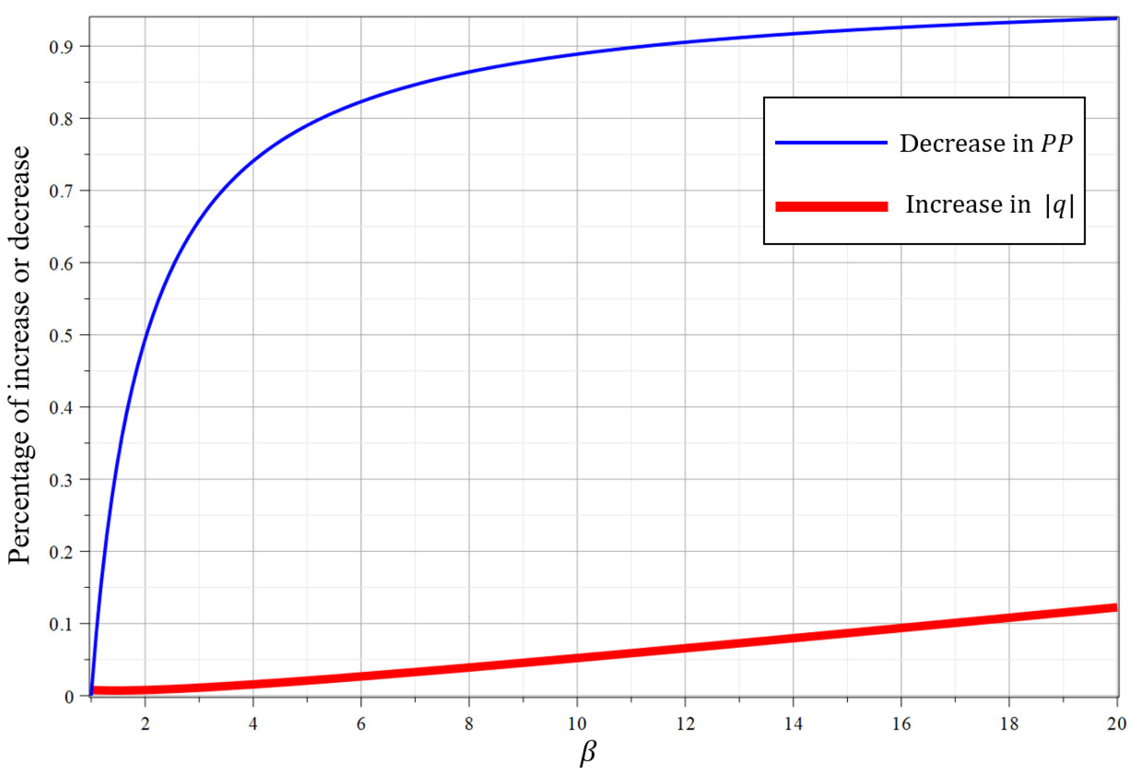
Trade-off. We make a trade-off between the decrease in the size of public parameters and the increase in the computation cost. Using the blocking technique, we divide an identity into segments, and the number of elements in public parameters is reduced from to where is a flexible constant. Therefore, the percentage of decrease in public parameter space is and it is shown as the thin blue line in Figure 1 with . According to the analysis of Singh [19], there is no effect of on cost of key generation, encryption and decription. However, we need to increase the value of lattice modulo q for maintaining the same security level, and it will increase the computation cost. According to Chatterjee ’s work [20], the number of bits in q is increased by . We use to denote the bit length of q and then . The percentage of increase in computation cost is and it is shown as the thick red line in Figure 1 with . In Figure 1, the x-axis represents the value of , and the y-axis represents the percentage of increase or decrease. For and , the size of public parameters is reduced by 89.7% while the cost of computation is merely increased by 5.2% when or . If we set or , the size of public parameters is reduced by 93.8% while the computational cost is merely increased by 12.25%.
Comparisons. We propose an adaptively secure IBE scheme in Section 3. Table 1 shows the comparison of storage space between different IBE schemes in the standard model. In this table, , , l denote the public parameters, private keys and length of user’s identity.
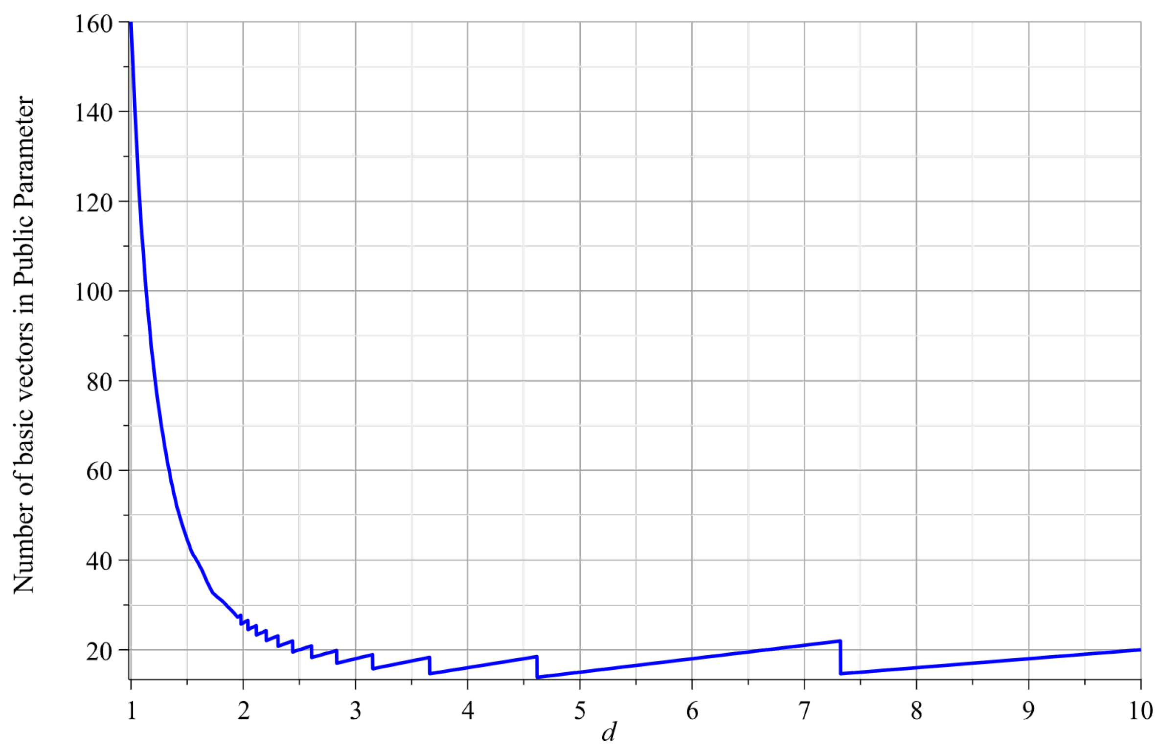
Since the public parameters are composed of multiple matrices, its size will directly affect the communication overhead in actual applications. As shown in this table, the public parameter in Agrawal’s construction [18] contains matrices. Zhang’s construction [23] achieves shorter public parameter at the cost of weaker security guarantees. In Yamada’s construction [22], the public parameter consists of matrices, where d is a constant. In Katsumata’s scheme [36], the public parameter consists of vectors because of ring setting. The relationship between the size of public parameters and constant d is shown in Figure 2. For , the minimum size of public parameters is 17 vectors when we set . Moreover, we need to set d very small (e.g., or 3) because of the reduction cost. If we set (resp. 3), the public parameters have 28 (resp. 20) vectors. In [24], the public parameter consists of matrices via new partitioning functions. In our construction, the public parameters only contain vectors, where . We have analyzed the choice of or in the previous part. For , the public parameter only contains 10 (resp. 18) vectors if we choose (resp. 10).
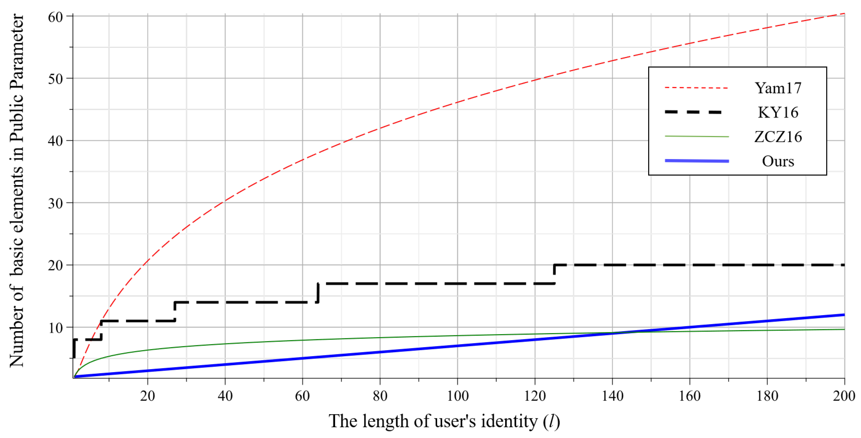
The comparison of public parameter size is shown in the Figure 3. It involves four IBE schemes with short public parameters, including Yam17 [24], KY16 [36] (), ZCZ16 [23] and ours (). The x-axis represents the length of user’s identity, and the y-axis represents the number of basic matrices (or vectors) in the public parameters of each scheme. Obviously, the public parameters in our scheme are shorter than [24] and [36]. Moreover, it can be shorter than [23] if the identity length l is small (e.g., less than 140).
Compared with the LWE-based scheme, the RLWE-based scheme contains a lot of polynomial operations instead of matrix operations. To compare more fair, we only compare the computational efficiency between the schemes under RLWE assumption. Since the scheme by [36] also has short public parameters and ring setting, we only compare the calculation efficiency between [36] and our scheme. Table 2 shows the comparison of computational efficiency. In this table, , , denote the key generation, encryption and decryption.
The difference between these two schemes is the calculation of and . In Katsumata’s construction [36], and it is used to generate private keys. They use the homomorphic function as in [22], which maps vectors to a vector in . The function needs multiplications and inversions. In our construction, and it is also used as the input of the sampling algorithm to generate private keys. However, it only needs multiplication operations which is obviously less than [36].
In Section 4, we also extend our IBE scheme to an adaptively secure HIBE scheme. Using Waters’ technology, we can convert the selectively secure HIBE scheme to adaptive security. Howerve, the size of the public parameter increases from matrices to matrices. In our HIBE construction, the public parameter is reduced from matrices to vectors where . In particular, it can be further reduced to thanks to the method of Chatterjee [11,43]. Finally, both of our constructions support multi-bit encryption because of ring setting.
6. Conclusions
In this paper, we propose an identity-based encryption scheme and a hierarchical identity-based encryption scheme over ideal lattice. The new schemes have short public parameters, and achieve IND-ID-CPA security in the standard model. In addition, we use the trapdoor of Micciancio to further improve the efficiency of our scheme. However, there are still many problems to be solved, such as how to reduce the size of ciphertext and how to implement these schemes.
Author Contributions
Conceptualization, S.Z.; Investigation, Y.G. and S.Z.; Methodology, Y.Z., Y.L., Y.G. and L.W.; Validation, Y.Z. and Y.L.; Writing—original draft, Y.Z.; Writing—review & editing, L.W. All authors have read and agreed to the published version of the manuscript.
Funding
This research was funded by Shandong Provincial Key Research and Development 512 Program of China: 2018CXGC0701; National Natural Science Foundation of China (NSFC): No. 61972050; BUPT Excellent Ph.D. Students Foundation: No. CX2019119 and in part by the 111 Project: No. B08004.
Conflicts of Interest
The authors declare no conflict of interest.
References
- Shamir, A. Identity-Based Cryptosystems and Signature Schemes. In Workshop on the Theory and Application of Cryptographic Techniques; Springer: Berlin/Heidelberger, Germany, 1984; pp. 47–53. [Google Scholar] [CrossRef] [Green Version]
- Boneh, D.; Franklin, M.K. Identity-Based Encryption from the Weil Pairing. In Annual International Cryptology Conference; Springer: Berlin/Heidelberger, Germany, 2001; pp. 213–229. [Google Scholar] [CrossRef] [Green Version]
- Canetti, R.; Halevi, S.; Katz, J. A Forward-Secure Public-Key Encryption Scheme. In International Conference on the Theory and Applications of Cryptographic Techniques; Springer: Berlin/Heidelberger, Germany, 2003; pp. 255–271. [Google Scholar] [CrossRef] [Green Version]
- Boneh, D.; Boyen, X. Secure Identity Based Encryption Without Random Oracles. In Annual International Cryptology Conference; Springer: Berlin/Heidelberger, Germany, 2004; pp. 443–459. [Google Scholar] [CrossRef] [Green Version]
- Waters, B. Efficient Identity-Based Encryption Without Random Oracles. In Annual International Conference on the Theory and Applications of Cryptographic Techniques; Springer: Berlin/Heidelberger, Germany, 2005; pp. 114–127. [Google Scholar] [CrossRef] [Green Version]
- Cocks, C.C. An Identity Based Encryption Scheme Based on Quadratic Residues. In IMA International Conference on Cryptography and Coding; Springer: Berlin/Heidelberger, Germany, 2001; pp. 360–363. [Google Scholar] [CrossRef]
- Gentry, C.; Silverberg, A. Hierarchical ID-Based Cryptography. In International Conference on the Theory and Application of Cryptology and Information Security; Springer: Berlin/Heidelberger, Germany, 2002; pp. 548–566. [Google Scholar] [CrossRef] [Green Version]
- Horwitz, J.; Lynn, B. Toward Hierarchical Identity-Based Encryption. In International Conference on the Theory and Applications of Cryptographic Techniques; Springer: Berlin/Heidelberger, Germany, 2002; pp. 466–481. [Google Scholar] [CrossRef] [Green Version]
- Boneh, D.; Boyen, X. Efficient Selective-ID Secure Identity-Based Encryption Without Random Oracles. In International Conference on the Theory and Applications of Cryptographic Techniques; Springer: Berlin/Heidelberger, Germany, 2004; pp. 223–238. [Google Scholar] [CrossRef] [Green Version]
- Gentry, C. Practical Identity-Based Encryption Without Random Oracles. In Annual International Conference on the Theory and Applications of Cryptographic Techniques; Springer: Berlin/Heidelberger, Germany, 2006; pp. 445–464. [Google Scholar] [CrossRef] [Green Version]
- Chatterjee, S.; Sarkar, P. HIBE With Short Public Parameters without Random Oracle. In International Conference on the Theory and Application of Cryptology and Information Security; Springer: Berlin/Heidelberger, Germany, 2006; pp. 145–160. [Google Scholar] [CrossRef] [Green Version]
- Canetti, R.; Halevi, S.; Katz, J. A Forward-Secure Public-Key Encryption Scheme. J. Cryptol. 2007, 20, 265–294. [Google Scholar] [CrossRef]
- Waters, B. Dual System Encryption: Realizing Fully Secure IBE and HIBE under Simple Assumptions. In Annual International Cryptology Conference; Springer: Berlin/Heidelberger, Germany, 2009; pp. 619–636. [Google Scholar] [CrossRef] [Green Version]
- Regev, O. On lattices, learning with errors, random linear codes, and cryptography. J. ACM 2005, 56, 1–40. [Google Scholar] [CrossRef]
- Stehlé, D.; Steinfeld, R.; Tanaka, K.; Xagawa, K. Efficient Public Key Encryption Based on Ideal Lattices. In International Conference on the Theory and Application of Cryptology and Information Security; Springer: Berlin/Heidelberger, Germany, 2009; pp. 617–635. [Google Scholar] [CrossRef] [Green Version]
- Lyubashevsky, V.; Peikert, C.; Regev, O. On Ideal Lattices and Learning with Errors over Rings. In Annual International Conference on the Theory and Applications of Cryptographic Techniques; Springer: Berlin/Heidelberger, Germany, 2010; pp. 1–23. [Google Scholar] [CrossRef]
- Gentry, C.; Peikert, C.; Vaikuntanathan, V. Trapdoors for hard lattices and new cryptographic constructions. In Proceedings of the 40th Annual ACM Symposium on Theory of Computing, Victoria, BC, Canada, 17–20 May 2008; pp. 197–206. [Google Scholar] [CrossRef] [Green Version]
- Agrawal, S.; Boneh, D.; Boyen, X. Efficient Lattice (H)IBE in the Standard Model. In Annual International Conference on the Theory and Applications of Cryptographic Techniques; Springer: Berlin/Heidelberger, Germany, 2010; pp. 553–572. [Google Scholar] [CrossRef] [Green Version]
- Singh, K.; Rangan, C.P.; Banerjee, A.K. Adaptively Secure Efficient Lattice (H)IBE in Standard Model with Short Public Parameters. In International Conference on Security, Privacy, and Applied Cryptography Engineering; Springer: Berlin/Heidelberger, Germany, 2012; pp. 153–172. [Google Scholar] [CrossRef]
- Chatterjee, S.; Sarkar, P. Trading Time for Space: Towards an Efficient IBE Scheme with Short(er) Public Parameters in the Standard Model. In International Conference on Information Security and Cryptology; Springer: Berlin/Heidelberger, Germany, 2005; pp. 424–440. [Google Scholar] [CrossRef]
- Naccache, D. Secure and practical identity-based encryption. IET Inf. Secur. 2005, 1, 59–64. [Google Scholar] [CrossRef] [Green Version]
- Yamada, S. Adaptively Secure Identity-Based Encryption from Lattices with Asymptotically Shorter Public Parameters. In Annual International Conference on the Theory and Applications of Cryptographic Techniques; Springer: Berlin/Heidelberger, Germany, 2016; pp. 32–62. [Google Scholar] [CrossRef]
- Zhang, J.; Chen, Y.; Zhang, Z. Programmable Hash Functions from Lattices: Short Signatures and IBEs with Small Key Sizes. In Annual international cryptology conference; Springer: Berlin/Heidelberger, Germany, 2016; pp. 303–332. [Google Scholar] [CrossRef]
- Yamada, S. Asymptotically Compact Adaptively Secure Lattice IBEs and Verifiable Random Functions via Generalized Partitioning Techniques. In Annual International Cryptology Conference; Springer: Berlin/Heidelberger, Germany, 2017; pp. 161–193. [Google Scholar] [CrossRef]
- Agrawal, S.; Boyen, X. Identity-Based Encryption from Lattices in the Standard Model. 2009. Available online: http://www.cs.stanford.edu/~xb/ab09/ (accessed on 20 October 2020).
- Cash, D.; Hofheinz, D.; Kiltz, E. How to Delegate a Lattice Basis. IACR Cryptol. ePrint Arch. 2009, 2009, 351. [Google Scholar]
- Cash, D.; Hofheinz, D.; Kiltz, E.; Peikert, C. Bonsai Trees, or How to Delegate a Lattice Basis. In Annual International Conference on the Theory and Applications of Cryptographic Techniques; Springer: Berlin/Heidelberger, Germany, 2010; pp. 523–552. [Google Scholar] [CrossRef] [Green Version]
- Agrawal, S.; Boneh, D.; Boyen, X. Lattice Basis Delegation in Fixed Dimension and Shorter-Ciphertext Hierarchical IBE. In Annual Cryptology Conference; Springer: Berlin/Heidelberger, Germany, 2010; pp. 98–115. [Google Scholar] [CrossRef] [Green Version]
- Wang, F.; Wang, C.; Liu, Z.H. Efficient hierarchical identity based encryption scheme in the standard model over lattices. Front. Inf. Technol. Electron. Eng. 2016, 17, 781–791. [Google Scholar] [CrossRef]
- Apon, D.; Fan, X.; Liu, F. Compact identity based encryption from LWE. Cryptol. ePrint Arch. 2016, 2016. [Google Scholar]
- Boyen, X.; Li, Q. Towards tightly secure lattice short signature and id-based encryption. In International Conference on the Theory and Application of Cryptology and Information Security; Springer: Berlin/Heidelberger, Germany, 2016; pp. 404–434. [Google Scholar]
- Zhang, L.; Wu, Q. Adaptively Secure Hierarchical Identity-Based Encryption over Lattice. In International Conference on Network and System Security; Springer: Berlin/Heidelberger, Germany, 2017; pp. 46–58. [Google Scholar] [CrossRef]
- Yang, X.; Wu, L.; Zhang, M.; Chen, X. An efficient CCA-secure cryptosystem over ideal lattices from identity-based encryption. Comput. Math. Appl. 2013, 65, 1254–1263. [Google Scholar] [CrossRef]
- Ducas, L.; Lyubashevsky, V.; Prest, T. Efficient Identity-Based Encryption over NTRU Lattices. In International Conference on the Theory and Application of Cryptology and Information Security; Springer: Berlin/Heidelberger, Germany, 2014; pp. 22–41. [Google Scholar] [CrossRef] [Green Version]
- Hoffstein, J.; Pipher, J.; Silverman, J.H. NTRU: A Ring-Based Public Key Cryptosystem. In ANTS-III; Springer: Berlin/Heidelberger, Germany, 1998; pp. 267–288. [Google Scholar] [CrossRef]
- Katsumata, S.; Yamada, S. Partitioning via Non-linear Polynomial Functions: More Compact IBEs from Ideal Lattices and Bilinear Maps. In International Conference on the Theory and Application of Cryptology and Information Security; Springer: Berlin/Heidelberger, Germany, 2016; pp. 682–712. [Google Scholar] [CrossRef]
- Bert, P.; Fouque, P.; Roux-Langlois, A.; Sabt, M. Practical Implementation of Ring-SIS/LWE Based Signature and IBE. In International Conference on Post-Quantum Cryptography; Springer: Berlin/Heidelberger, Germany, 2018; pp. 271–291. [Google Scholar] [CrossRef] [Green Version]
- Micciancio, D.; Peikert, C. Trapdoors for Lattices: Simpler, Tighter, Faster, Smaller. In Annual International Conference on the Theory and Applications of Cryptographic Techniques; Springer: Berlin/Heidelberger, Germany, 2012; pp. 700–718. [Google Scholar] [CrossRef] [Green Version]
- Peikert, C. Bonsai Trees (or, Arboriculture in Lattice-Based Cryptography). IACR Cryptol. ePrint Arch. 2009, 2009, 359. [Google Scholar]
- Ajtai, M. Generating Hard Instances of Lattice Problems (Extended Abstract). In Proceedings of the Twenty-Eighth Annual ACM Symposium on the Theory of Computing, Philadelphia, PA, USA, 22–24 May 1996; pp. 99–108. [Google Scholar] [CrossRef]
- Banaszczyk, W. New bounds in some transference theorems in the geometry of numbers. Math. Ann. 1993, 296, 625–635. [Google Scholar] [CrossRef]
- Banaszczyk, W. Inequalites for Convex Bodies and Polar Reciprocal Lattices in Rn. Discret. Comput. Geom. 1995, 13, 217–231. [Google Scholar] [CrossRef]
- Singh, K.; Rangan, C.P.; Banerjee, A.K. Efficient Lattice HIBE in the Standard Model with Shorter Public Parameters. In Information and Communication Technology-EurAsia Conference; Springer: Berlin/Heidelberger, Germany, 2014; pp. 542–553. [Google Scholar] [CrossRef] [Green Version]
Figure 1.
Relative decrease in and relative increase in .

Figure 2.
The relationship between the size of public parameters and constant d.

Figure 3.
Comparison of public parameter size in different schemes.


Table 1.
Comparison of storage space.
| Schemes | Size | Size | Ciphertext Size | Security | Assumption |
|---|---|---|---|---|---|
| [18] | Adaptive-CPA | LWE | |||
| [23] | Adaptive-CPA | LWE | |||
| [22] * | Adaptive-CPA | LWE | |||
| [36] * | Adaptive-CPA | RLWE † | |||
| [24] | Adaptive-CPA | LWE | |||
| Ours ** | Adaptive-CPA | RLWE † |
* In [22] and [36], they use an injective map which maps an identity to a subset of , where the element d is a flexible constant. The choice of d will affect the reduction cost; ** In our construction, the element is a flexible constant. The choice of will affect the size of modulus q and we make a trade-off in the previous part; † Our scheme and [36] only work over the rings ; thus, the basic elements in the public parameters are polynomial vectors rather than matrices.
Table 2.
Comparison of computational efficiency.
| Schemes | |||
|---|---|---|---|
| [36] | |||
| Ours |
Publisher’s Note: MDPI stays neutral with regard to jurisdictional claims in published maps and institutional affiliations. |
© 2020 by the authors. Licensee MDPI, Basel, Switzerland. This article is an open access article distributed under the terms and conditions of the Creative Commons Attribution (CC BY) license (http://creativecommons.org/licenses/by/4.0/).
Share and Cite
MDPI and ACS Style
Zhang, Y.; Liu, Y.; Guo, Y.; Zheng, S.; Wang, L. Adaptively Secure Efficient (H)IBE over Ideal Lattice with Short Parameters. Entropy 2020, 22, 1247. https://0-doi-org.brum.beds.ac.uk/10.3390/e22111247
AMA Style
Zhang Y, Liu Y, Guo Y, Zheng S, Wang L. Adaptively Secure Efficient (H)IBE over Ideal Lattice with Short Parameters. Entropy. 2020; 22(11):1247. https://0-doi-org.brum.beds.ac.uk/10.3390/e22111247
Chicago/Turabian StyleZhang, Yuan, Yuan Liu, Yurong Guo, Shihui Zheng, and Licheng Wang. 2020. "Adaptively Secure Efficient (H)IBE over Ideal Lattice with Short Parameters" Entropy 22, no. 11: 1247. https://0-doi-org.brum.beds.ac.uk/10.3390/e22111247
Note that from the first issue of 2016, this journal uses article numbers instead of page numbers. See further details here.