
A Novel Conflict Management Method Based on Uncertainty of Evidence and Reinforcement Learning for Multi-Sensor Information Fusion


Abstract
:1. Introduction
- The negation of evidence is introduced into RL to achieve information quality assessment. The uncertainty of original evidence and its negation is obtained by using Deng entropy. Then, the obtained uncertainty degrees are used to distinguish the information quality of evidence, which helps to realize the access to information.
- In order to achieve the adaptive online information fusion, RL is combined with the uncertainty degrees to process the conflicting evidence. In this process, a Markov decision process (MDP) model is built, and solved through Q-learning algorithm to implement the fusion of evidence.
2. Preliminaries
2.1. Dempster–Shafer Theory (DST)
2.2. Negation of Evidence
2.3. Deng Entropy
2.4. Correlation Coefficient
2.5. Reinforcement Learning (RL)
3. The Proposed Method
3.1. Markov Decision Process (MDP)
3.1.1. Action Set
3.1.2. State Set
3.1.3. Reward
3.2. Q-Learning Algorithm Solution
| Algorithm 1 The proposed evidence combination algorithm. |
|
3.3. Decision Making Based on Correlation Coefficient
4. Simulation Analysis and Application
4.1. Numerical Example
4.1.1. Numerical Example 1
4.1.2. Numerical Example 2
4.2. Application to Fault Diagnosis and Analysis
4.2.1. Application to Fault Diagnosis
4.2.2. Robustness Analysis
5. Conclusions
Author Contributions
Funding
Institutional Review Board Statement
Informed Consent Statement
Data Availability Statement
Conflicts of Interest
References
- Ramírez-Gallego, S.; Fernández, A.; García, S.; Chen, M.; Herrera, F. Big data: Tutorial and guidelines on information and process fusion for analytics algorithms with mapreduce. Inf. Fusion 2018, 42, 51–61. [Google Scholar] [CrossRef]
- Xiao, F. Multi-sensor data fusion based on the belief divergence measure of evidences and the belief entropy. Inf. Fusion 2019, 46, 23–32. [Google Scholar] [CrossRef]
- Xiao, F. CEQD: A complex mass function to predict interference effects. IEEE Trans. Cybern. 2021, 99, 1–13. [Google Scholar]
- Zhen, Z.; Jiang, J.; Wang, X.; Gao, C. Information fusion based optimal control for large civil aircraft system. ISA Trans. 2015, 55, 81–91. [Google Scholar] [CrossRef] [PubMed]
- Li, D.; Deng, Y.; Cheong, K. Multi-source basic probability assignment fusion based on information quality. Int. J. Intell. Syst. 2021, 36, 1851–1875. [Google Scholar] [CrossRef]
- Mahfouz, A.; Adnan, M.; Gerhard, P. Localised information fusion techniques for location discovery in wireless sensor networks. Int. J. Sens. Netw. 2018, 26, 12. [Google Scholar] [CrossRef] [Green Version]
- He, Y.; Zhai, D.; Jiang, Y.; Zhang, R. Relay selection for UAV-assisted urban vehicular ad hoc networks. IEEE Wirel. Commun. Lett. 2020, 9, 1379–1383. [Google Scholar] [CrossRef]
- He, Y.; Zhai, D.; Huang, F.; Wang, D.; Tang, X.; Zhang, R. Joint task offloading, resource allocation, and security assurance for mobile edge computing-enabled UAV-assisted VANETs. Remote Sens. 2021, 13, 1547. [Google Scholar] [CrossRef]
- Habbouche, H.; Benkedjouh, T.; Amirat, Y.; Benbouzid, M. Gearbox Failure Diagnosis Using a Multisensor Data-Fusion Machine-Learning-Based Approach. Entropy 2021, 23, 697. [Google Scholar] [CrossRef]
- Ullah, K.; Mahmood, T.; Garg, H. Evaluation of the performance of search and rescue robots using T-spherical fuzzy hamacher aggregation operators. Int. J. Fuzzy Syst. 2020, 22, 570–582. [Google Scholar] [CrossRef]
- Fu, C.; Chang, W.; Liu, W.; Yang, S. Data-driven group decision making for diagnosis of thyroid nodule. Sci. China Inf. Sci. 2019, 62, 212205. [Google Scholar] [CrossRef] [Green Version]
- Fu, C.; Chang, W.; Xue, M.; Yang, S. Multiple criteria group decision making with belief distributions and distributed preference relations. Eur. J. Oper. Res. 2019, 273, 623–633. [Google Scholar] [CrossRef]
- Xiao, F. A new divergence measure for belief functions in D–S evidence theory for multi sensor data fusion. Inf. Sci. 2020, 514, 462–483. [Google Scholar] [CrossRef]
- Deng, J.; Deng, Y.; Cheong, K. Combining Conflicting Evidence Based on Pearson Correlation Coefficient and Weighted Graph. Int. J. Intell. Syst. 2021, 4, 1–18. [Google Scholar]
- Liao, H.; Ren, Z.; Fang, R. A Deng-Entropy-Based Evidential Reasoning Approach for Multi-expert Multi-criterion Decision-Making with Uncertainty. Int. J. Comput. Intell. Syst. 2020, 13, 1281–1294. [Google Scholar] [CrossRef]
- Kang, B.; Deng, Y.; Hewage, K.; Sadiq, R. A method of measuring uncertainty for Z-number. IEEE Trans. Fuzzy Syst. 2019, 27, 731–738. [Google Scholar] [CrossRef]
- Tian, Y.; Liu, L.; Mi, X.; Kang, B. ZSLF: A new soft likelihood function based on z-numbers and its application in expert decision system. IEEE Trans. Fuzzy Syst. 2020, 22, 2333–2349. [Google Scholar] [CrossRef]
- Deng, X.; Jiang, W. A total uncertainty measure for D numbers based on belief intervals. Int. J. Intell. Syst. 2019, 34, 3302–3316. [Google Scholar] [CrossRef] [Green Version]
- Xiao, F. A multiple criteria decision-making method based on D numbers and belief entropy. Int. J. Fuzzy Syst. 2019, 21, 1144–1153. [Google Scholar] [CrossRef]
- Zadeh, L.A. Fuzzy sets. Inf. Control 1965, 8, 338–353. [Google Scholar] [CrossRef] [Green Version]
- Ullah, K.; Garg, H.; Mahmood, T.; Jan, N.; Ali, Z. Correlation coefficients for T-spherical fuzzy sets and their applications in clustering and multi-attribute decision making. Soft Comput. 2020, 24, 1647–1659. [Google Scholar] [CrossRef]
- Xiao, F. CaFtR: A Fuzzy Complex Event Processing Method. Int. J. Fuzzy Syst. 2021, 38, 1–14. [Google Scholar]
- Greco, S.; Matarazzo, B.; Slowinski, R. Rough sets theory for multicriteria decision analysis. Eur. J. Oper. Res. 2001, 129, 1–47. [Google Scholar] [CrossRef]
- Ding, W.; Lin, C.T.; Prasad, M. Hierarchical co-evolutionary clustering tree-based rough feature game equilibrium selection and its application in neonatal cerebral cortex MRI. Expert Syst. Appl. 2018, 101, 243–257. [Google Scholar] [CrossRef]
- Seiti, H.; Hafezalkotob, A.; Martínez, L. R-numbers, a new risk modeling associated with fuzzy numbers and its application to decision making. Inf. Sci. 2019, 483, 206–231. [Google Scholar] [CrossRef]
- Gao, X.; Deng, Y. The pseudo-pascal triangle of maximum Deng entropy. Int. J. Comput. Commun. Control 2020, 15, 1–10. [Google Scholar] [CrossRef] [Green Version]
- Zhang, J.; Liu, R.; Zhang, J.; Kang, B. Extension of Yager’s negation of a probability distribution based on tsallis entropy. Int. J. Intell. Syst 2020, 35, 72–84. [Google Scholar] [CrossRef]
- Shafer, G. A Mathematical Theory of Evidence; Princeton University Press: Princeton, NJ, USA, 1976. [Google Scholar]
- Dempster, A.P. Upper and lower probabilities induced by a multivalued mapping. Ann. Math. Stat. 1967, 38, 325–339. [Google Scholar] [CrossRef]
- Zadeh, L.A. A simple view of the Dempster-Shafer theory of evidence and its implication for the rule of combination. AI Mag. 1986, 7, 85–90. [Google Scholar]
- Yager, R. On the Dempster–Shafer framework and new combination rules. Inf. Sci. 1987, 41, 93–137. [Google Scholar] [CrossRef]
- Dubois, D.; Prade, H. Representation and combination of uncertainty with belief functions and possibility measures. Comput. Intell. 1988, 4, 244–264. [Google Scholar] [CrossRef]
- Murphy, C. Combining belief functions when evidence conflicts. Decis. Support Syst. 2000, 29, 1–9. [Google Scholar] [CrossRef]
- Lefevre, E.; Colot, O.; Vannoorenberghe, P. Belief functions combination and conflict management. Inf. Fusion 2002, 3, 149–162. [Google Scholar] [CrossRef]
- Smets, P. Analyzing the combination of conflicting belief functions. Inf. Fusion 2007, 8, 387–412. [Google Scholar] [CrossRef]
- Dezert, J.; Smarandache, F. Advances and Applications of DSmT for Information Fusion; American Research Press: Rehoboth, MA, USA, 2015. [Google Scholar]
- Song, Y.; Wang, X.; Lei, L.; Yue, S. Uncertainty measure for interval-valued belief structures. Measurement 2016, 80, 241–250. [Google Scholar] [CrossRef]
- Wang, X.; Zhu, J.; Song, Y.; Lei, L. Combination of unreliable evidence sources in intuitionistic fuzzy MCDM framework. Knowl. Based Syst. 2016, 97, 24–39. [Google Scholar] [CrossRef] [Green Version]
- Yuan, K.; Xiao, F.; Fei, L.; Kang, B.; Deng, Y. Conflict management based on belief function entropy in sensor fusion. SpringerPlus 2016, 5, 638. [Google Scholar] [CrossRef] [PubMed] [Green Version]
- Deng, Y. Deng entropy. Chaos Solitons Fractals 2016, 91, 549–553. [Google Scholar] [CrossRef]
- Jousselme, A.; Grenier, D.; Bossé, É. A new distance between two bodies of evidence. Inf. Fusion 2001, 2, 91–101. [Google Scholar] [CrossRef]
- Jiang, W.; Wei, B.; Xie, C.; Zhou, D. An evidential sensor fusion method in fault diagnosis. Adv. Mech. Eng. 2016, 8, 1–7. [Google Scholar] [CrossRef] [Green Version]
- Ni, S.; Lei, Y.; Tang, Y. Improved base belief function-based conflict data fusion approach considering belief entropy in the evidence theory. Entropy 2020, 22, 801. [Google Scholar] [CrossRef]
- Smets, P. The application of the matrix calculus to belief functions. Int. J. Approx. Reason. 2002, 31, 1–30. [Google Scholar] [CrossRef] [Green Version]
- Deng, X.; Jiang, W. On the negation of a Dempster–Shafer belief structure based on maximum uncertainty allocation. Inf. Sci. 2020, 516, 346–352. [Google Scholar] [CrossRef] [Green Version]
- Mao, H.; Deng, Y. Negation of BPA: A belief interval approach and its application in medical pattern recognition. Appl. Intell. 2021, 43, 1–18. [Google Scholar]
- Yin, L.; Deng, X.; Deng, Y. The Negation of a Basic Probability Assignment. IEEE Trans. Fuzzy Syst. 2018, 27, 135–143. [Google Scholar] [CrossRef]
- Xie, K.; Xiao, F. Negation of Belief Function Based on the Total Uncertainty Measure. Entropy 2019, 21, 73. [Google Scholar] [CrossRef] [Green Version]
- Shannon, C.E. A mathematical theory of communication. Bell Syst. Tech. J. 1948, 27, 379–423. [Google Scholar] [CrossRef] [Green Version]
- Jiang, W. A correlation coefficient for belief functions. Int. J. Approx. Reason. 2018, 103, 94–106. [Google Scholar] [CrossRef] [Green Version]
- Mahmud, M.; Kaiser, M.; Hussain, A.; Vassanelli, S. Applications of deep learning and reinforcement learning to biological data. IEEE Trans. Neural Netw. Learn. Syst. 2017, 29, 2063–2079. [Google Scholar] [CrossRef] [Green Version]
- Saha, T.; Gupta, D.; Saha, S.; Bhattacharyya, P. Towards integrated dialogue policy learning for multiple domains and intents using hierarchical deep reinforcement learning. Expert Syst. Appl. 2020, 162, 113650. [Google Scholar] [CrossRef]
- Chen, Y.; Norford, L.; Samuelson, H.; Malkawi, A. Optimal control of HV AC and window systems for natural ventilation through reinforcement learning. Energy Build. 2018, 169, 195–205. [Google Scholar] [CrossRef]
- Jiang, W.; Xie, C.; Zhuang, M.; Shou, Y. Sensor data dusion with Z-Numbers and its application in fault diagnosis. Sensors 2016, 16, 1509. [Google Scholar] [CrossRef] [PubMed]
- Pal, N.R.; Bezdek, J.C.; Hemasinha, R. Uncertainty measures for evidential reasoning I: A review. Int. J. Approx. Reason. 1992, 7, 165–183. [Google Scholar] [CrossRef] [Green Version]
- Pal, N.R.; Bezdek, J.C.; Hemasinha, R. Uncertainty measures for evidential reasoning II: A new measure of total uncertainty. Int. J. Approx. Reason. 1993, 8, 1–16. [Google Scholar] [CrossRef] [Green Version]


| BPA | ||||
|---|---|---|---|---|
| Sensor 1: | 0.41 | 0.29 | 0.30 | 0 |
| Sensor 2: | 0 | 0.90 | 0.10 | 0 |
| Sensor 3: | 0.58 | 0.07 | 0 | 0.35 |
| Sensor 4: | 0.55 | 0.10 | 0 | 0.35 |
| Sensor 5: | 0.60 | 0.10 | 0 | 0.30 |
| Parameter | Value |
|---|---|
| Discount factor () | 0.9 |
| Learning rate () | 0.1 |
| Episode number (M) | 100 |
| BPA | Sensor 1: | Sensors 2: | Sensor 3: | Sensor 4: | Sensor 5: |
| Processing result | Retain | Delete | Retain | Retain | Retain |
| The Negation of BPA | |||
|---|---|---|---|
| 0.41 | 0.29 | 0.30 | |
| 0 | 0.8969 | 0.1031 | |
| 0.9213 | 0.0787 | 0 | |
| 0.9847 | 0.0153 | 0 | |
| 0.9974 | 0.0026 | 0 |
| Methods | |||||||
|---|---|---|---|---|---|---|---|
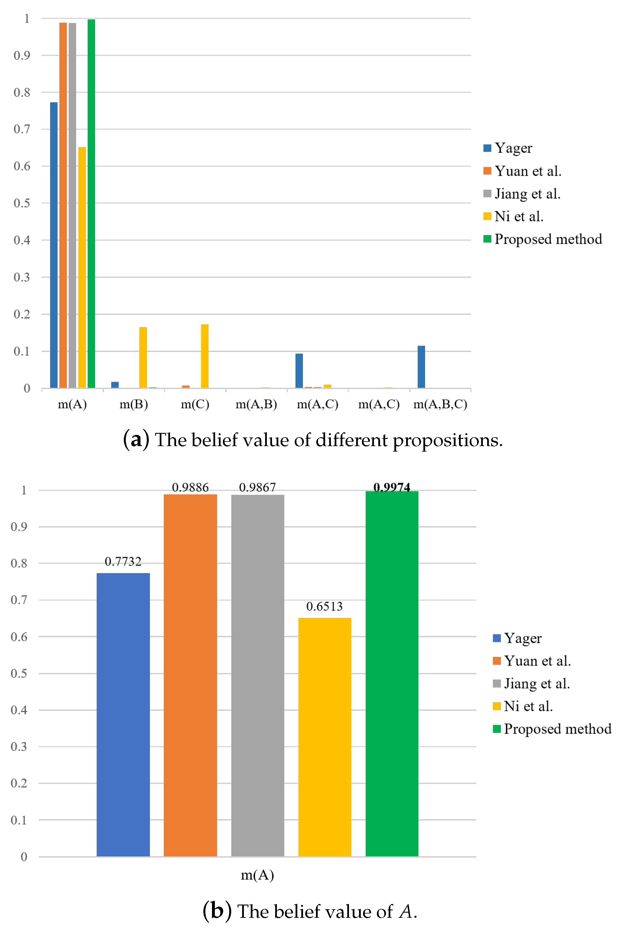
| Yager [31] | 0.7732 | 0.0167 | 0.0011 | 0 | 0.0938 | 0 | 0.1152 |
| Yuan et al. [39] | 0.9886 | 0.0002 | 0.0072 | 0 | 0.0039 | 0 | 0 |
| Jiang et al. [42] | 0.9867 | 0.0008 | 0 | 0 | 0.0036 | 0 | 0 |
| Ni et al. [43] | 0.6513 | 0.1648 | 0.1730 | 0.0016 | 0.0096 | 0.0016 | 0 |
| Proposed method | 0.9974 | 0.0026 | 0 | 0 | 0 | 0 | 0 |
| Methods | Decision-Making Result | |||
|---|---|---|---|---|
| Yager [31] | 0.9750 | 0.0532 | 0.0716 | A |
| Yuan et al. [39] | 1 | 0.0002 | 0.0086 | A |
| Jiang et al. [42] | 1 | 0.0008 | 0.0012 | A |
| Ni et al. [43] | 0.9378 | 0.2375 | 0.2530 | A |
| Proposed method | 1 | 0.0026 | 0 | A |
| BPA | |||||
|---|---|---|---|---|---|
| 0.7 | 0 | 0 | 0.3 | 0 | |
| 0.4 | 0 | 0 | 0.3 | 0.3 | |
| 0.55 | 0.2 | 0.05 | 0 | 0.2 |
| The Negation of BPA | ||||
|---|---|---|---|---|
| 0.7 | 0 | 0 | 0.30 | |
| 0.7722 | 0.1139 | 0 | 0.1139 | |
| 0.8209 | 0.1791 | 0 | 0 | |
| 0.8425 | 0.1575 | 0 | 0 | |
| (a) BPAs for the application under feature 1. | ||||
| BPA | ||||
| Sensor 1: | 0.8176 | 0.0003 | 0.1553 | 0.0268 |
| Sensor 2: | 0.5658 | 0.0009 | 0.0646 | 0.3687 |
| Sensor 3: | 0.2403 | 0.0004 | 0.0141 | 0.7452 |
| (b) BPAs for the application under feature 2. | ||||
| BPA | ||||
| Sensor 1: | 0.6229 | 0.3771 | ||
| Sensor 2: | 0.7660 | 0.2340 | ||
| Sensor 3: | 0.8598 | 0.1402 | ||
| (c) BPAs for the application under feature 3. | ||||
| BPA | ||||
| Sensor 1: | 0.3666 | 0.4563 | 0.1185 | 0.0586 |
| Sensor 2: | 0.2793 | 0.4151 | 0.2652 | 0.0404 |
| Sensor 3: | 0.2897 | 0.4331 | 0.2470 | 0.0302 |
| Parameter | Value |
|---|---|
| Discount factor () | 0.9 |
| Learning rate () | 0.1 |
| Episode number (M) | 80 |
| BPA | The First Round of Processing Results | The Final Round of Processing Results | |
|---|---|---|---|
| Feature 1 | Sensor 1: | Retain | Retain |
| Sensor 2: | Retain | Retain | |
| Sensor 3: | Waiting to Process | Delete | |
| Feature 2 | Sensor 1: | Retain | Retain |
| Sensor 2: | Retain | Retain | |
| Sensor 3: | Retain | Retain | |
| Feature 3 | Sensor 1: | Retain | Retain |
| Sensor 2: | Retain | Retain | |
| Sensor 3: | Retain | Retain | |
| (a) The negation of the BPAs for the application under feature 1. | |||
| The Negation of BPA | |||
| 0.8176 | 0.0003 | 0.1821 | |
| 0.9587 | 0 | 0.0432 | |
| 0.9368 | 0 | 0.0632 | |
| (b) The negation of the BPAs for the application under feature 2. | |||
| The Negation of BPA | |||
| 0.6229 | 0.3771 | ||
| 0.8440 | 0.1562 | ||
| 0.9708 | 0.0292 | ||
| (c) The negation of the BPAs for the application under feature 3. | |||
| The Negation of BPA | |||
| 0.3666 | 0.4563 | 0.1771 | |
| 0.3145 | 0.5817 | 0.1038 | |
| 0.2482 | 0.6863 | 0.0655 | |
| (a) Fusion results of different methods for the application under feature 1. | |||||||
| Methods | |||||||
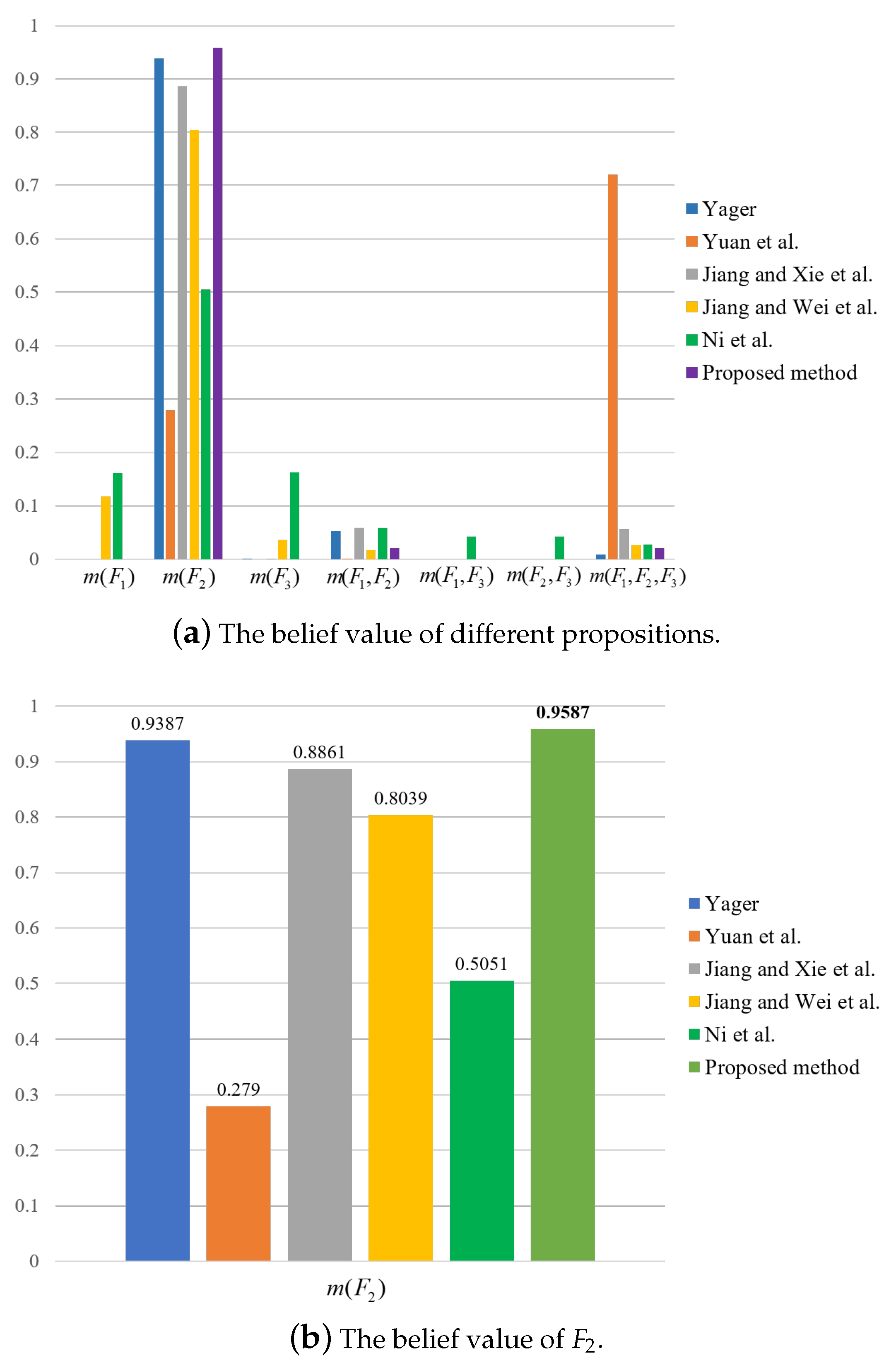
| Yager [31] | 0 | 0.9387 | 0.0001 | 0.0526 | 0 | 0 | 0.0086 |
| Yuan et al. [39] | 0 | 0.2790 | 0 | 0.0003 | 0 | 0 | 0.7207 |
| Jiang and Xie et al. [54] | 0 | 0.8861 | 0.0002 | 0.0582 | 0 | 0 | 0.0555 |
| Jiang and Wei et al. [42] | 0.1178 | 0.8039 | 0.0356 | 0.0170 | 0 | 0 | 0.0257 |
| Ni et al. [43] | 0.1616 | 0.5051 | 0.1619 | 0.0587 | 0.0425 | 0.0425 | 0.0276 |
| Proposed method | 0 | 0.9587 | 0 | 0.0208 | 0 | 0 | 0.0205 |
| (b) Fusion results of different methods for the application under feature 2. | |||||||
| Methods | |||||||
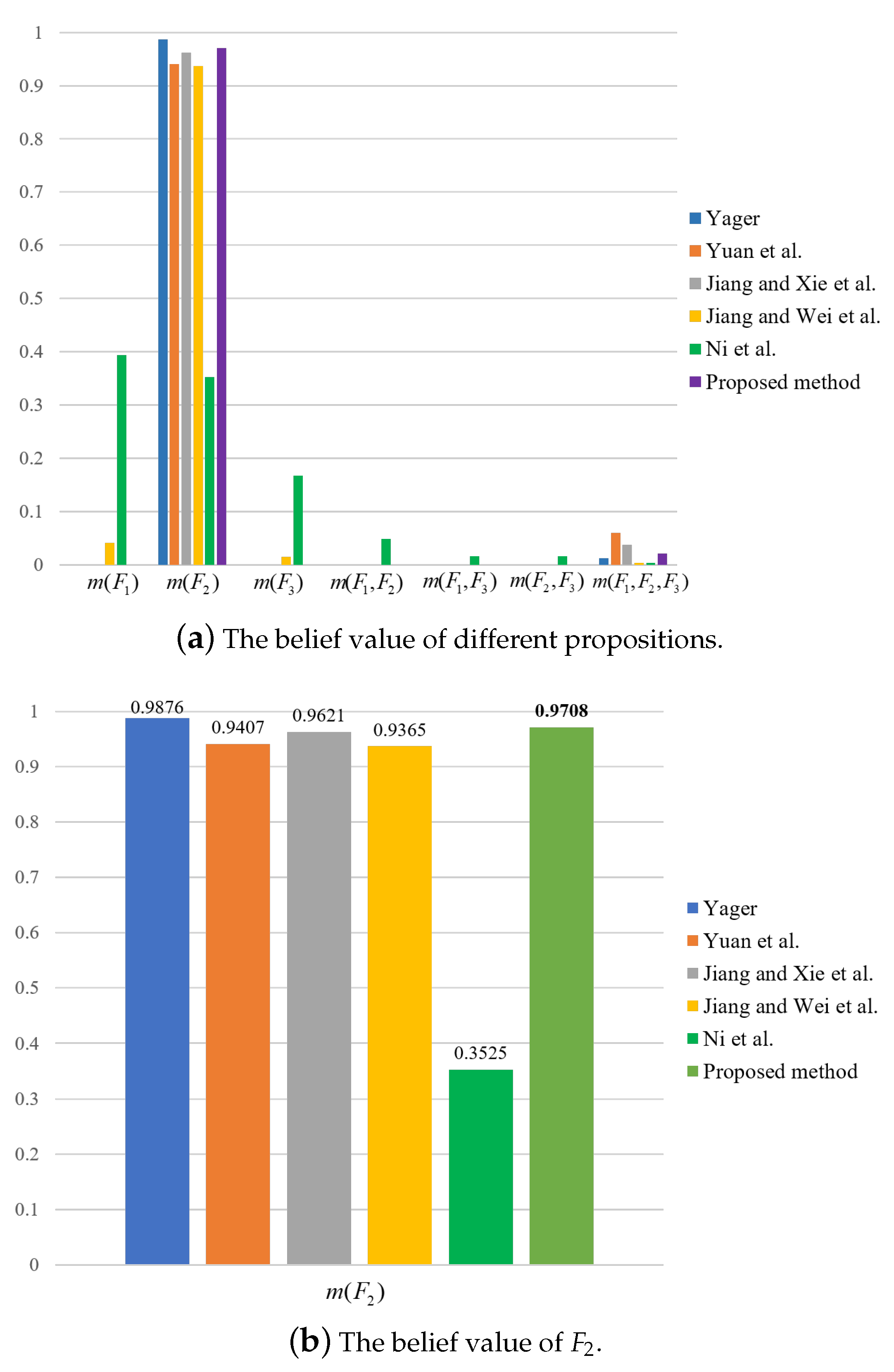
| Yager [31] | 0 | 0.9876 | 0 | 0 | 0 | 0 | 0.0124 |
| Yuan et al. [39] | 0 | 0.9407 | 0 | 0 | 0 | 0 | 0.0593 |
| Jiang and Xie et al. [54] | 0 | 0.9621 | 0 | 0 | 0 | 0 | 0.0371 |
| Jiang and Wei et al. [42] | 0.0461 | 0.9365 | 0.0144 | 0 | 0 | 0 | 0.0030 |
| Ni et al. [43] | 0.3938 | 0.3525 | 0.1679 | 0.0487 | 0.0162 | 0.0162 | 0.0030 |
| Proposed method | 0 | 0.9708 | 0 | 0 | 0 | 0 | 0.0292 |
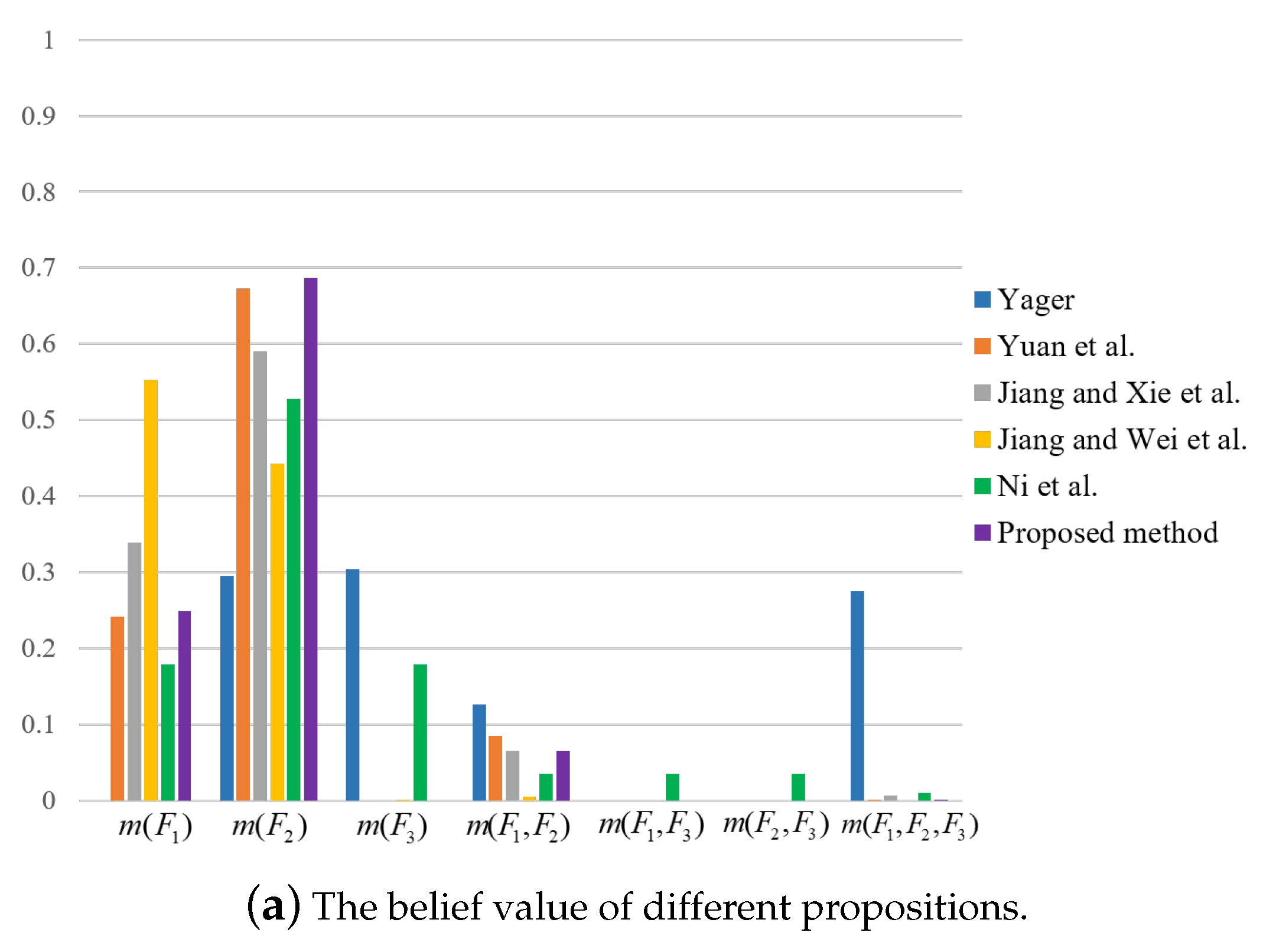
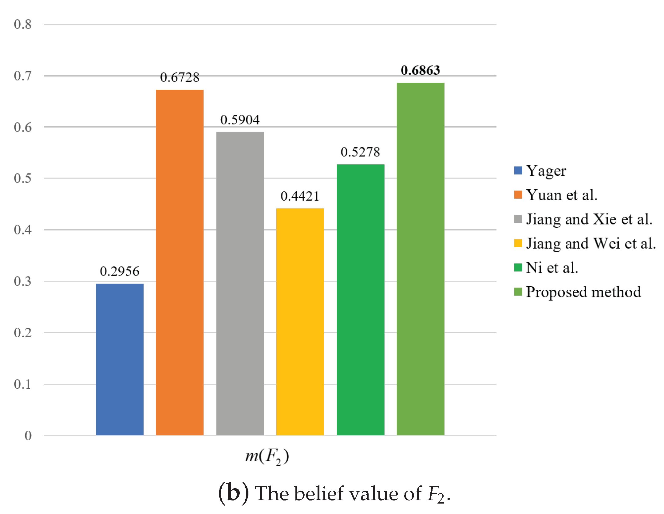
| (c) Fusion results of different methods for the application under feature 3. | |||||||
| Methods | |||||||
| Yager [31] | 0 | 0.2956 | 0.3034 | 0.1260 | 0 | 0 | 0.2750 |
| Yuan et al. [39] | 0.2414 | 0.6728 | 0 | 0.0852 | 0 | 0 | 0.0006 |
| Jiang and Xie et al. [54] | 0.3384 | 0.5904 | 0 | 0.0651 | 0 | 0 | 0.0061 |
| Jiang and Wei et al. [42] | 0.4421 | 0.5528 | 0.0005 | 0.0046 | 0 | 0 | 0 |
| Ni et al. [43] | 0.1787 | 0.5278 | 0.1787 | 0.0348 | 0.0348 | 0.0348 | 0.0097 |
| Proposed method | 0.2482 | 0.6863 | 0 | 0.0649 | 0 | 0 | 0.0006 |
| (a) The correlation value under feature 1. | ||||
| Methods | Decision-Making Result | |||
| Yager [31] | 0.0205 | 0.9983 | 0.0023 | |
| Yuan et al. [39] | 0.2158 | 0.5497 | 0.2156 | |
| Jiang and Xie et al. [54] | 0.0360 | 0.9940 | 0.0152 | |
| Jiang and Wei et al. [42] | 0.1569 | 0.9854 | 0.0507 | |
| Ni et al. [43] | 0.3225 | 0.8700 | 0.3141 | |
| Proposed method | 0.0124 | 0.9993 | 0.0053 | |
| (b) The correlation value under feature 2. | ||||
| Methods | Decision-Making Result | |||
| Yager [31] | 0.0031 | 0.9999 | 0.0031 | |
| Yuan et al. [39] | 0.0155 | 0.9982 | 0.0155 | |
| Jiang and Xie et al. [54] | 0.0095 | 0.9993 | 0.0095 | |
| Jiang and Wei et al. [42] | 0.0499 | 0.9986 | 0.0161 | |
| Ni et al. [43] | 0.7036 | 0.6337 | 0.3034 | |
| Proposed method | 0 | 0.9996 | 0.0099 | |
| (c) The correlation value under feature 3. | ||||
| Methods | Decision-Making Result | |||
| Yager [31] | 0.1689 | 0.5675 | 0.6196 | |
| Yuan et al. [39] | 0.3574 | 0.9286 | 0.0002 | |
| Jiang and Xie et al. [54] | 0.5058 | 0.8583 | 0.0021 | |
| Jiang and Wei et al. [42] | 0.6248 | 0.7807 | 0.0007 | |
| Ni et al. [43] | 0.3244 | 0.8787 | 0.3244 | |
| Proposed method | 0.3552 | 0.9317 | 0.0002 | |
| No. | BPA | Conflict Degree | |||||
|---|---|---|---|---|---|---|---|
| 1 | Sensor 1: | 0 | 0.8176 | 0.0003 | 0.1553 | 0.0268 | |
| Sensor 2: | 0 | 0.5658 | 0.0009 | 0.0646 | 0.3687 | ||
| Sensor 3: | 0 | 0.2403 | 0.0004 | 0.0141 | 0.7452 | ||
| 2 | Sensor 1: | 0 | 0.8176 | 0.0003 | 0.1553 | 0.0268 | |
| Sensor 2: | 0 | 0.5158 | 0.0509 | 0.0646 | 0.3687 | ||
| Sensor 3: | 0.05 | 0.2403 | 0.0004 | 0.0141 | 0.6952 | ||
| 3 | Sensor 1: | 0 | 0.8176 | 0.0003 | 0.1553 | 0.0268 | |
| Sensor 2: | 0 | 0.4658 | 0.1009 | 0.0646 | 0.3687 | ||
| Sensor 3: | 0.1 | 0.2403 | 0.0004 | 0.0141 | 0.6452 | ||
| 4 | Sensor 1: | 0 | 0.8176 | 0.0003 | 0.1553 | 0.0268 | |
| Sensor 2: | 0 | 0.4158 | 0.1509 | 0.0646 | 0.3687 | ||
| Sensor 3: | 0.15 | 0.2403 | 0.0004 | 0.0141 | 0.5952 | ||
| 5 | Sensor 1: | 0 | 0.8176 | 0.0003 | 0.1553 | 0.0268 | |
| Sensor 2: | 0 | 0.3658 | 0.2009 | 0.0646 | 0.3687 | ||
| Sensor 3: | 0.2 | 0.2403 | 0.0004 | 0.0141 | 0.5452 | ||
| 6 | Sensor 1: | 0 | 0.8176 | 0.0003 | 0.1553 | 0.0268 | |
| Sensor 2: | 0 | 0.3158 | 0.2509 | 0.0646 | 0.3687 | ||
| Sensor 3: | 0.25 | 0.2403 | 0.0004 | 0.0141 | 0.4952 | ||
| 7 | Sensor 1: | 0 | 0.8176 | 0.0003 | 0.1553 | 0.0268 | |
| Sensor 2: | 0 | 0.2658 | 0.3009 | 0.0646 | 0.3687 | ||
| Sensor 3: | 0.3 | 0.2403 | 0.0004 | 0.0141 | 0.4452 | ||
| 8 | Sensor 1: | 0 | 0.8176 | 0.0003 | 0.1553 | 0.0268 | |
| Sensor 2: | 0 | 0.2158 | 0.3509 | 0.0646 | 0.3687 | ||
| Sensor 3: | 0.35 | 0.2403 | 0.0004 | 0.0141 | 0.3952 |
| No. | BPA | Conflict Degree | ||||
|---|---|---|---|---|---|---|
| 1 | Sensor 1: | 0 | 0.6229 | 0 | 0.3771 | |
| Sensor 2: | 0 | 0.7660 | 0 | 0.2340 | ||
| Sensor 3: | 0 | 0.8598 | 0 | 0.1402 | ||
| 2 | Sensor 1: | 0.05 | 0.5729 | 0 | 0.3771 | |
| Sensor 2: | 0 | 0.7160 | 0.05 | 0.2340 | ||
| Sensor 3: | 0 | 0.8598 | 0 | 0.1402 | ||
| 3 | Sensor 1: | 0.1 | 0.5229 | 0 | 0.3771 | |
| Sensor 2: | 0 | 0.6660 | 0.1 | 0.2340 | ||
| Sensor 3: | 0 | 0.8598 | 0 | 0.1402 | ||
| 4 | Sensor 1: | 0.15 | 0.4729 | 0 | 0.3771 | |
| Sensor 2: | 0 | 0.6160 | 0.15 | 0.2340 | ||
| Sensor 3: | 0 | 0.8598 | 0 | 0.1402 | ||
| 5 | Sensor 1: | 0.2 | 0.4229 | 0 | 0.3771 | |
| Sensor 2: | 0 | 0.5660 | 0.2 | 0.2340 | ||
| Sensor 3: | 0 | 0.8598 | 0 | 0.1402 | ||
| 6 | Sensor 1: | 0.25 | 0.3729 | 0 | 0.3771 | |
| Sensor 2: | 0 | 0.5160 | 0.25 | 0.2340 | ||
| Sensor 3: | 0 | 0.8598 | 0 | 0.1402 | ||
| 7 | Sensor 1: | 0.3 | 0.3229 | 0 | 0.3771 | |
| Sensor 2: | 0 | 0.4660 | 0.3 | 0.2340 | ||
| Sensor 3: | 0 | 0.8598 | 0 | 0.1402 | ||
| 8 | Sensor 1: | 0.35 | 0.2729 | 0 | 0.3771 | |
| Sensor 2: | 0 | 0.4160 | 0.35 | 0.2340 | ||
| Sensor 3: | 0 | 0.8598 | 0 | 0.1402 |
| No. | BPA | Conflict Degree | |||||
|---|---|---|---|---|---|---|---|
| 1 | Sensor 1: | 0.3666 | 0.4563 | 0 | 0.1185 | 0.0586 | |
| Sensor 2: | 0.2793 | 0.4151 | 0 | 0.2652 | 0.0404 | ||
| Sensor 3: | 0.2897 | 0.4331 | 0 | 0.2470 | 0.0302 | ||
| 2 | Sensor 1: | 0.3666 | 0.4563 | 0 | 0.1185 | 0.0586 | |
| Sensor 2: | 0.3093 | 0.4151 | 0 | 0.2352 | 0.0404 | ||
| Sensor 3: | 0.2897 | 0.4331 | 0.03 | 0.2170 | 0.0302 | ||
| 3 | Sensor 1: | 0.3666 | 0.4563 | 0 | 0.1185 | 0.0586 | |
| Sensor 2: | 0.3393 | 0.4151 | 0 | 0.2052 | 0.0404 | ||
| Sensor 3: | 0.2897 | 0.4331 | 0.06 | 0.1870 | 0.0302 | ||
| 4 | Sensor 1: | 0.3666 | 0.4563 | 0 | 0.1185 | 0.0586 | |
| Sensor 2: | 0.3693 | 0.4151 | 0 | 0.1752 | 0.0404 | ||
| Sensor 3: | 0.2897 | 0.4331 | 0.09 | 0.1570 | 0.0302 | ||
| 5 | Sensor 1: | 0.3666 | 0.4563 | 0 | 0.1185 | 0.0586 | |
| Sensor 2: | 0.3993 | 0.4151 | 0 | 0.1452 | 0.0404 | ||
| Sensor 3: | 0.2897 | 0.4331 | 0.12 | 0.1270 | 0.0302 | ||
| 6 | Sensor 1: | 0.3666 | 0.4563 | 0 | 0.1185 | 0.0586 | |
| Sensor 2: | 0.4293 | 0.4151 | 0 | 0.1152 | 0.0404 | ||
| Sensor 3: | 0.2897 | 0.4331 | 0.15 | 0.0970 | 0.0302 | ||
| 7 | Sensor 1: | 0.3666 | 0.4563 | 0 | 0.1185 | 0.0586 | |
| Sensor 2: | 0.4593 | 0.4151 | 0 | 0.0852 | 0.0404 | ||
| Sensor 3: | 0.2897 | 0.4331 | 0.18 | 0.0670 | 0.0302 | ||
| 8 | Sensor 1: | 0.3666 | 0.4563 | 0 | 0.1185 | 0.0586 | |
| Sensor 2: | 0.4893 | 0.4151 | 0 | 0.0552 | 0.0404 | ||
| Sensor 3: | 0.2897 | 0.4331 | 0.21 | 0.0370 | 0.0302 |
| (a) Fusion results under feature 1. | |||||||
| No. | |||||||
| 1 | 0 | 0.9587 | 0 | 0.0208 | 0 | 0 | 0.0205 |
| 2 | 0 | 0.9549 | 0 | 0.0227 | 0 | 0 | 0.0224 |
| 3 | 0 | 0.9502 | 0 | 0.0251 | 0 | 0 | 0.0247 |
| 4 | 0 | 0.9445 | 0 | 0.0279 | 0 | 0 | 0.0276 |
| 5 | 0 | 0.9374 | 0.0002 | 0.0314 | 0 | 0 | 0.0314 |
| 6 | 0 | 0.9281 | 0.0003 | 0.0361 | 0 | 0 | 0.0355 |
| 7 | 0 | 0.9200 | 0 | 0.0025 | 0 | 0 | 0.0775 |
| 8 | 0 | 0.9129 | 0 | 0.0030 | 0 | 0 | 0.0841 |
| (b) Fusion results under feature 2. | |||||||
| No. | |||||||
| 1 | 0 | 0.9708 | 0 | 0 | 0 | 0 | 0.0292 |
| 2 | 0 | 0.9661 | 0 | 0 | 0 | 0 | 0.0339 |
| 3 | 0 | 0.9603 | 0 | 0 | 0 | 0 | 0.0397 |
| 4 | 0 | 0.9529 | 0 | 0 | 0 | 0 | 0.0471 |
| 5 | 0 | 0.9433 | 0 | 0 | 0 | 0 | 0.0567 |
| 6 | 0 | 0.9304 | 0 | 0 | 0 | 0 | 0.0696 |
| 7 | 0 | 0.9127 | 0 | 0 | 0 | 0 | 0.0873 |
| 8 | 0 | 0.8875 | 0 | 0 | 0 | 0 | 0.1125 |
| (c) Fusion results under feature 3. | |||||||
| No. | |||||||
| 1 | 0.2482 | 0.6863 | 0 | 0.0649 | 0 | 0 | 0.0006 |
| 2 | 0.2715 | 0.6780 | 0 | 0.0500 | 0 | 0 | 0.0005 |
| 3 | 0.2837 | 0.6686 | 0 | 0.0371 | 0 | 0 | 0.0006 |
| 4 | 0.3148 | 0.6585 | 0 | 0.0262 | 0 | 0 | 0.0005 |
| 5 | 0.3347 | 0.6475 | 0 | 0.0172 | 0 | 0 | 0.0006 |
| 6 | 0.3534 | 0.6358 | 0 | 0.0103 | 0 | 0 | 0.0005 |
| 7 | 0.3708 | 0.6235 | 0 | 0.0051 | 0 | 0 | 0.0006 |
| 8 | 0.3869 | 0.6108 | 0 | 0.0018 | 0 | 0 | 0.0005 |
Publisher’s Note: MDPI stays neutral with regard to jurisdictional claims in published maps and institutional affiliations. |
© 2021 by the authors. Licensee MDPI, Basel, Switzerland. This article is an open access article distributed under the terms and conditions of the Creative Commons Attribution (CC BY) license (https://creativecommons.org/licenses/by/4.0/).
Share and Cite
Huang, F.; Zhang, Y.; Wang, Z.; Deng, X. A Novel Conflict Management Method Based on Uncertainty of Evidence and Reinforcement Learning for Multi-Sensor Information Fusion. Entropy 2021, 23, 1222. https://0-doi-org.brum.beds.ac.uk/10.3390/e23091222
Huang F, Zhang Y, Wang Z, Deng X. A Novel Conflict Management Method Based on Uncertainty of Evidence and Reinforcement Learning for Multi-Sensor Information Fusion. Entropy. 2021; 23(9):1222. https://0-doi-org.brum.beds.ac.uk/10.3390/e23091222
Chicago/Turabian StyleHuang, Fanghui, Yu Zhang, Ziqing Wang, and Xinyang Deng. 2021. "A Novel Conflict Management Method Based on Uncertainty of Evidence and Reinforcement Learning for Multi-Sensor Information Fusion" Entropy 23, no. 9: 1222. https://0-doi-org.brum.beds.ac.uk/10.3390/e23091222