
Numerical Simulation of Nocturnal Ozone Increase in Metropolitan Area of São Paulo †

 ,
, 
Abstract
:1. Introduction
2. Methodology
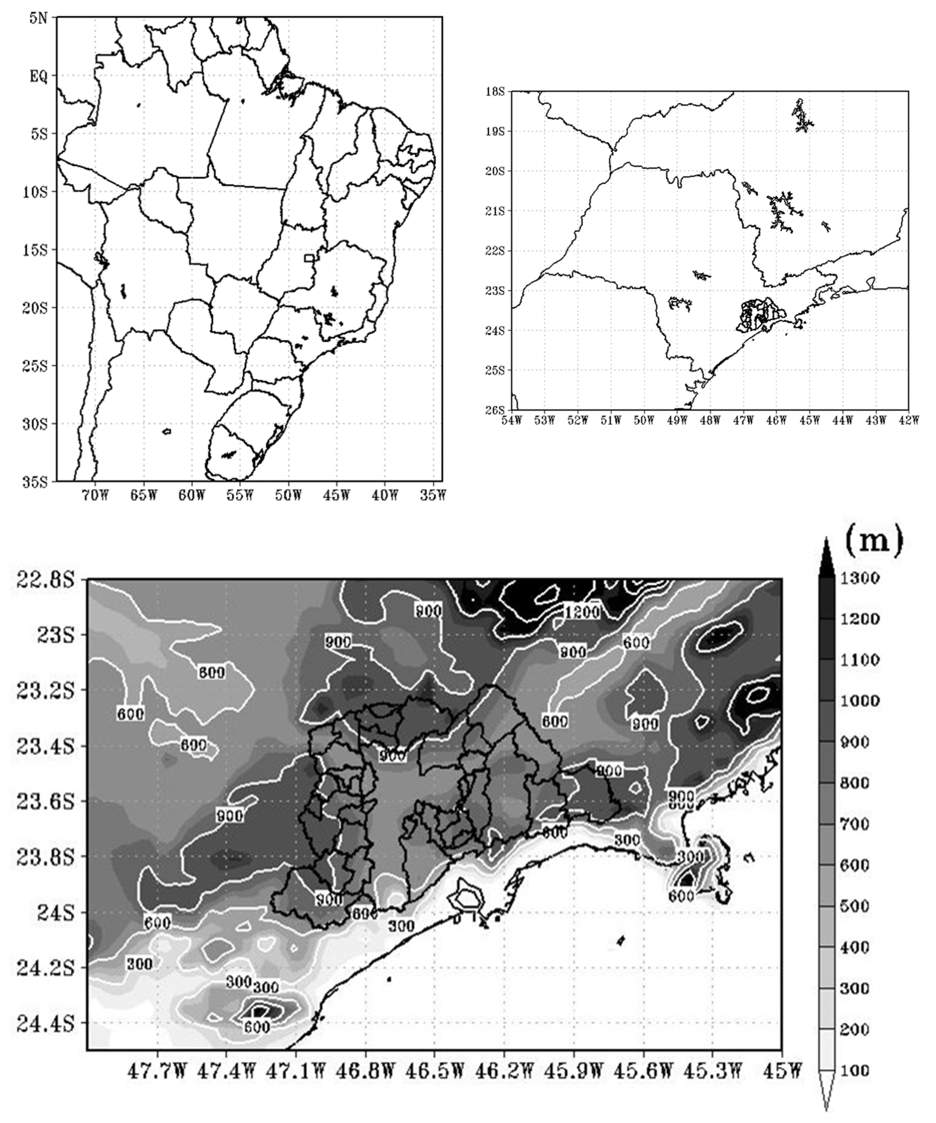
2.1. Study Area
2.2. SPM-BRAMS
2.3. Model Evaluation
2.4. Experimental Design
3. Results and Discussions
3.1. Model Evaluation
3.2. Nocturnal Ozone Experiments
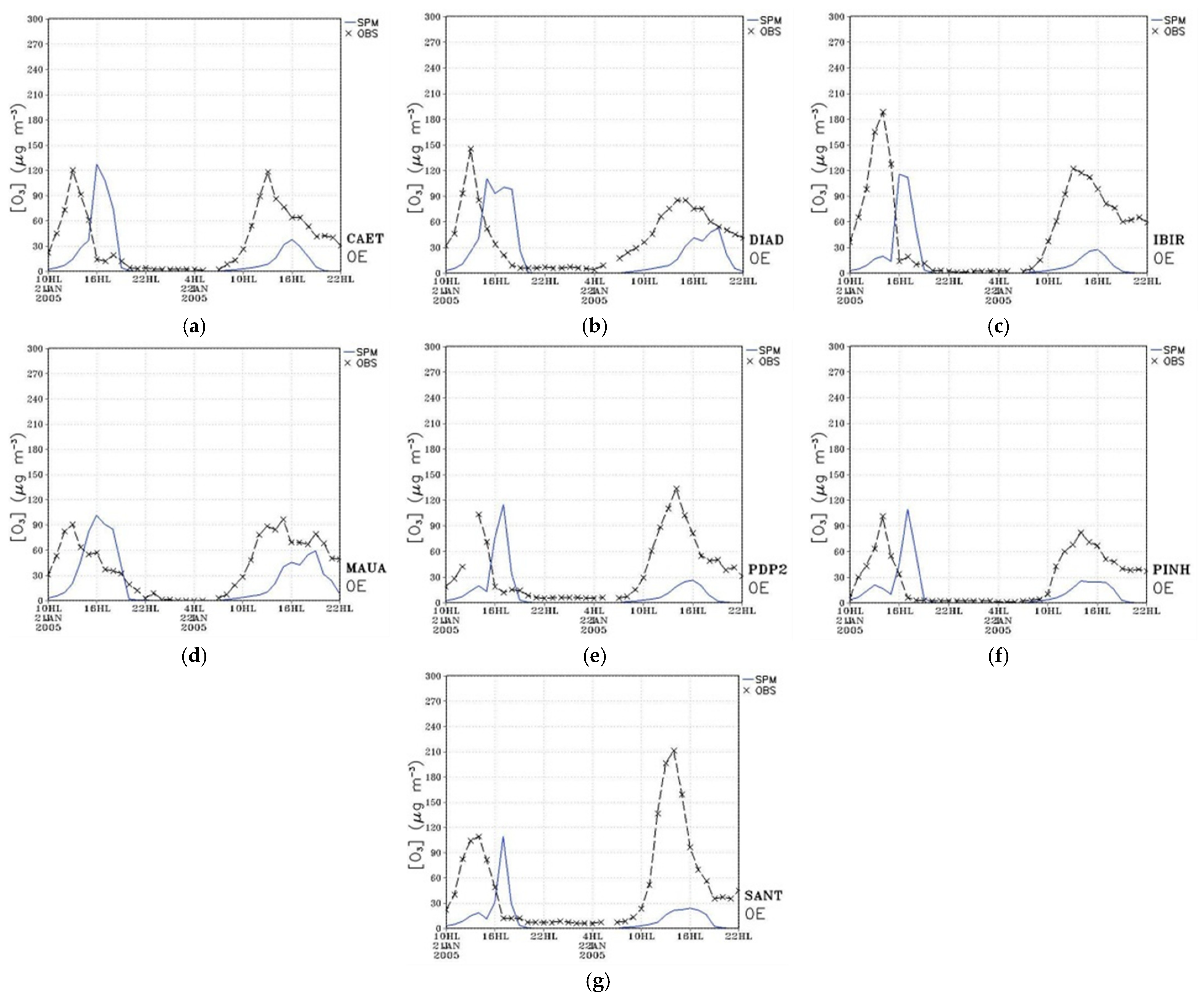
3.2.1. No Increase in Ozone Concentration (0E)
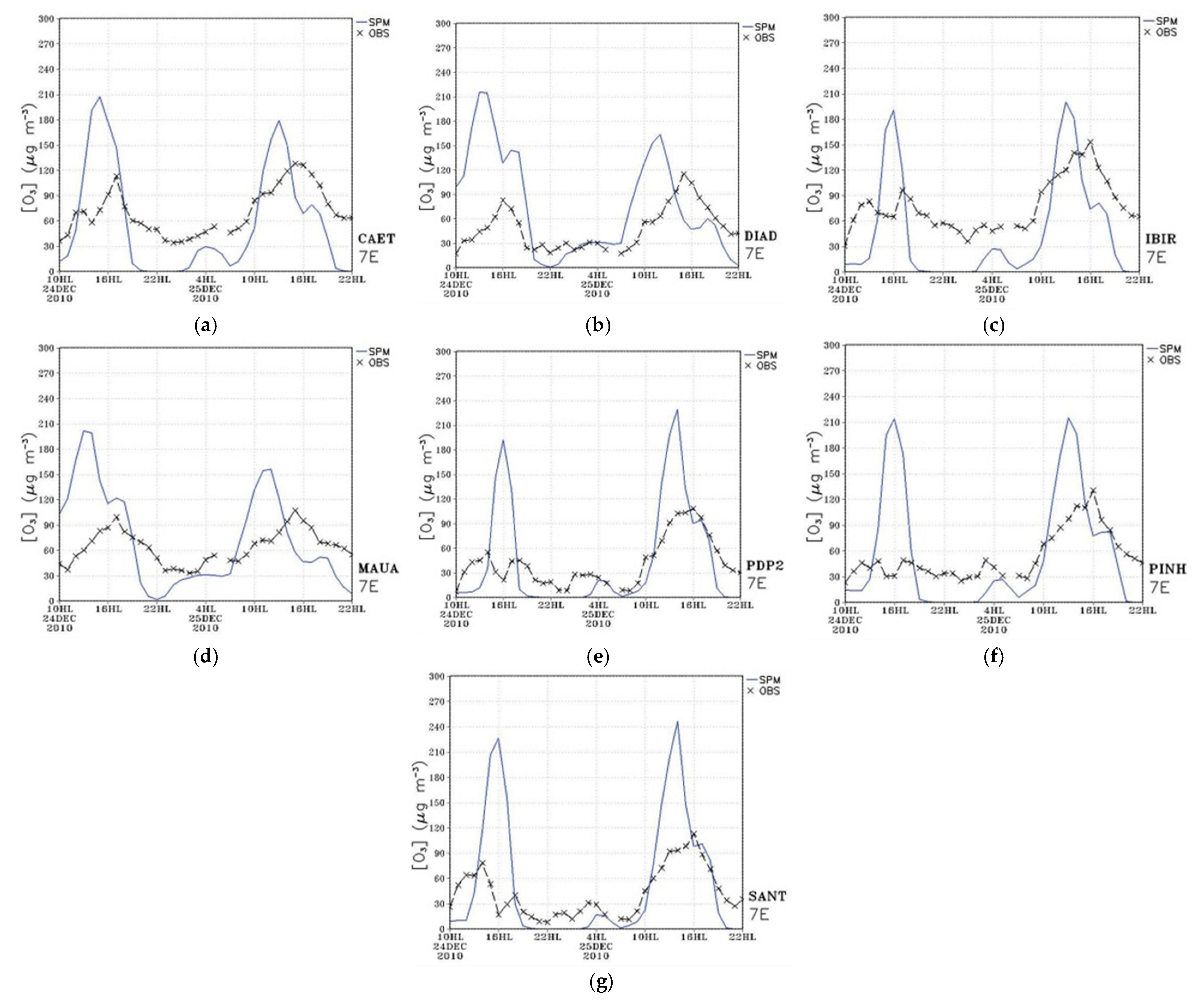
3.2.2. Increase in Ozone Concentration (7E)
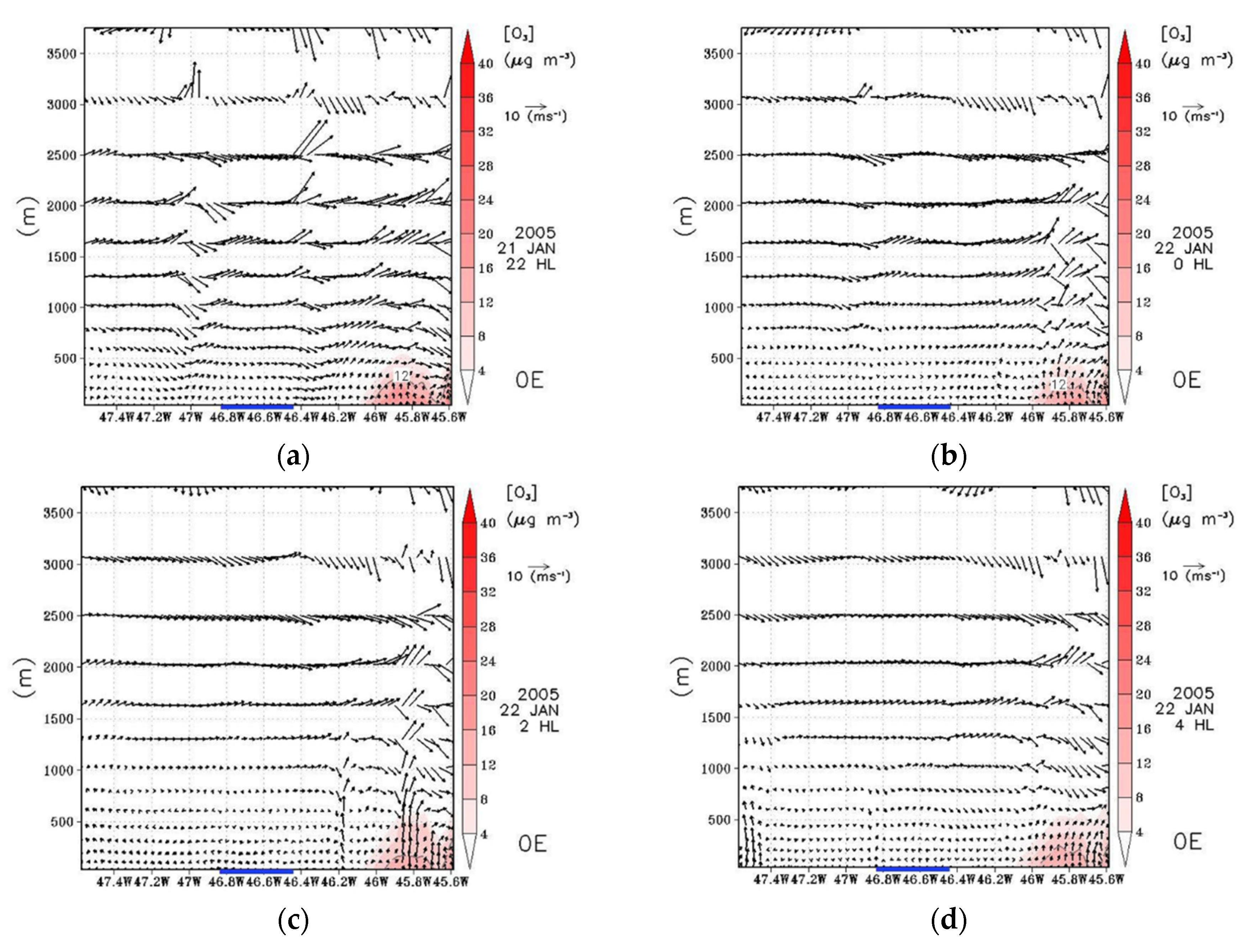
3.2.3. Ozone Vertical Profile
4. Conclusions and Remarks
Author Contributions
Funding
Conflicts of Interest
References
- Liana, M.; Edison, O.; Jorge, M.; Marcos, M.; Leda, A.; Guerrero, U.; Leila, M.D. Current state of air quality in major cities of Latin America. Ciência e Nat. 2016, 38, 523–531. [Google Scholar] [CrossRef]
- Patz, J.A.; Campbell-Lendrum, D.; Holloway, T.; Foley, J.A. Impact of regional climate change on human health. Nature 2005, 438, 310–317. [Google Scholar] [CrossRef]
- Woodall, G.M.; Hoover, M.D.; Williams, R.; Benedict, K.; Harper, M.; Soo, J.C.; Jarabek, A.M.; Stewart, M.J.; Brown, J.S.; Hulla, J.E.; et al. Interpreting mobile and handheld air sensor readings in relation to air quality standards and health effect reference values: Tackling the challenges. Atmosphere 2017, 8, 182. [Google Scholar] [CrossRef]
- Bell, M.L.; Zanobetti, A.; Dominici, F. Who is More Affected by Ozone Pollution? A Systematic Review and Meta-Analysis. Am. J. Epidemiol. 2014, 180, 15–28. [Google Scholar] [CrossRef]
- Wang, T.; Kwok, J.Y.H. Measurement and Analysis of a Multiday Photochemical Smog Episode in the Pearl River Delta of China. J. Appl. Meteorol. 2003, 42, 404–416. [Google Scholar] [CrossRef]
- Andrade, M.D.F.; Ynoue, R.Y.; Freitas, E.D.; Todesco, E.; Vara Vela, A.; Ibarra, S.; Martins, L.D.; Martins, J.A.; Carvalho, V.S.B. Air quality forecasting system for Southeastern Brazil. Front. Environ. Sci. 2015, 3, 1–14. [Google Scholar] [CrossRef]
- Samaali, M.; Moran, M.D.; Bouchet, V.S.; Pavlovic, R.; Cousineau, S.; Sassi, M. On the influence of chemical initial and boundary conditions on annual regional air quality model simulations for North America. Atmos. Environ. 2009, 43, 4873–4885. [Google Scholar] [CrossRef]
- Balzarini, A.; Pirovano, G.; Honzak, L.; Žabkar, R.; Curci, G.; Forkel, R.; Hirtl, M.; San José, R.; Tuccella, P.; Grell, G.A. WRF-Chem model sensitivity to chemical mechanisms choice in reconstructing aerosol optical properties. Atmos. Environ. 2015, 115, 604–619. [Google Scholar] [CrossRef]
- Vara-Vela, A.; Andrade, M.F.; Kumar, P.; Ynoue, R.Y.; Muñoz, A.G. Impact of vehicular emissions on the formation of fine particles in the Sao Paulo Metropolitan Area: A numerical study with the WRF-Chem model. Atmos. Chem. Phys. 2016, 16, 777–797. [Google Scholar] [CrossRef]
- Romero, H.; Ihl, M.; Rivera, A.; Zalazar, P.; Azocar, P. Rapid urban growth, land-use changes and air pollution in Santiago, Chile. Atmos. Environ. 1999, 33, 4039–4047. [Google Scholar] [CrossRef]
- Mar, K.A.; Ojha, N.; Pozzer, A.; Butler, T.M. Ozone air quality simulations with WRF-Chem (v3.5.1) over Europe: Model evaluation and chemical mechanism comparison. Geosci. Model Dev. Discuss. 2016, 1, 1–50. [Google Scholar] [CrossRef]
- Ren, X.; Mi, Z.; Georgopoulos, P.G. Comparison of Machine Learning and Land Use Regression for fine scale spatiotemporal estimation of ambient air pollution: Modeling ozone concentrations across the contiguous United States. Environ. Int. 2020, 142, 105827. [Google Scholar] [CrossRef] [PubMed]
- Gramsch, E.; Cereceda-Balic, F.; Oyola, P.; von Baer, D. Examination of pollution trends in Santiago de Chile with cluster analysis of PM10 and Ozone data. Atmos. Environ. 2006, 40, 5464–5475. [Google Scholar] [CrossRef]
- Khan, B.A.; de Freitas, C.R.; Shooter, D. Application of synoptic weather typing to an investigation of nocturnal ozone concentration at a maritime location, New Zealand. Atmos. Environ. 2007, 41, 5636–5646. [Google Scholar] [CrossRef]
- Alp, K.; Hanedar, A.O. Determination of transport processes of nocturnal ozone in Istanbul atmosphere. Int. J. Environ. Pollut. 2009, 39, 213. [Google Scholar] [CrossRef]
- Zhu, X.; Ma, Z.; Li, Z.; Wu, J.; Guo, H.; Yin, X.; Ma, X.; Qiao, L. Impacts of meteorological conditions on nocturnal surface ozone enhancement during the summertime in Beijing. Atmos. Environ. 2020, 225, 117368. [Google Scholar] [CrossRef]
- IBGE Censo Demográfico: Características da População—Mostra. Available online: https://censo2010.ibge.gov.br/resultados.html (accessed on 16 October 2020).
- Nair, K.N.; Freitas, E.D.; Snchez-Ccoyllo, O.R.; Silva Dias, M.a.F.; Silva Dias, P.L.; Andrade, M.F.; Massambani, O. Dynamics of urban boundary layer over São Paulo associated with mesoscale processes. Meteorol. Atmos. Phys. 2004, 86, 87–98. [Google Scholar] [CrossRef]
- Andrade, M.d.F.; Kumar, P.; de Freitas, E.D.; Ynoue, R.Y.; Martins, J.; Martins, L.D.; Nogueira, T.; Perez-Martinez, P.; de Miranda, R.M.; Albuquerque, T.; et al. Air quality in the megacity of São Paulo: Evolution over the last 30 years and future perspectives. Atmos. Environ. 2017, 159, 66–82. [Google Scholar] [CrossRef]
- Freitas, S.R.; Panetta, J.; Longo, K.M.; Rodrigues, L.F.; Moreira, D.S.; Rosário, N.E.; Silva Dias, P.L.; Silva Dias, M.A.F.; Souza, E.P.; Freitas, E.D.; et al. The Brazilian developments on the Regional Atmospheric Modeling System (BRAMS 5.2): An integrated environmental model tuned for tropical areas. Geosci. Model Dev. 2017, 10, 189–222. [Google Scholar] [CrossRef]
- Cotton, W.R.; Pielke Sr., R.a.; Walko, R.L.; Liston, G.E.; Tremback, C.J.; Jiang, H.; McAnelly, R.L.; Harrington, J.Y.; Nicholls, M.E.; Carrio, G.G.; et al. RAMS 2001: Current status and future directions. Meteorol. Atmos. Phys. 2003, 82, 5–29. [Google Scholar] [CrossRef]
- Walko, R.L.; Band, L.E.; Baron, J.; Kittel, T.G.F.; Lammers, R.; Lee, T.J.; Ojima, D.; Pielke, R.A.; Taylor, C.; Tague, C.; et al. Coupled Atmosphere–Biophysics–Hydrology Models for Environmental Modeling. J. Appl. Meteorol. 2000, 39, 931–944. [Google Scholar] [CrossRef]
- Masson, V. A physically-based scheme for the urban energy budget in atmospheric models. Bound.-Layer Meteorol. 2000, 94, 357–397. [Google Scholar] [CrossRef]
- Daley, R. (Ed.) Atmospheric Data Analysis; Cambridge University Press: Cambridge, UK, 1991. [Google Scholar]
- Morais, M.V.B.; Freitas, E.D.; Marciotto, E.R.; Urbina Guerrero, V.V.; Martins, L.D.; Martins, J.A. Implementation of observed sky-view factor in a mesoscale model for sensitivity studies of the urban meteorology. Sustainability 2018, 10, 2183. [Google Scholar] [CrossRef]
- Freitas, E.D.; Martins, L.D.; Silva Dias, P.L.; Andrade, M.F. A simple photochemical module implemented in RAMS for tropospheric ozone concentration forecast in the metropolitan area of São Paulo, Brazil: Coupling and validation. Atmos. Environ. 2005, 39, 6352–6361. [Google Scholar] [CrossRef]
- Wang, L.; Zhang, Y.; Wang, K.; Zheng, B.; Zhang, Q.; Wei, W. Application of Weather Research and Forecasting Model with Chemistry (WRF/Chem) over northern China: Sensitivity study, comparative evaluation, and policy implications. Atmos. Environ. 2014. [Google Scholar] [CrossRef]
- de Morais, M.V.B.; de Freitas, E.D.; Urbina Guerrero, V.V.; Martins, L.D. A modeling analysis of urban canopy parameterization representing the vegetation effects in the megacity of São Paulo. Urban Clim. 2016, 17, 102–115. [Google Scholar] [CrossRef]
- Pellegatti Franco, D.M.; Andrade, M.d.F.; Ynoue, R.Y.; Ching, J. Effect of Local Climate Zone (LCZ) classification on ozone chemical transport model simulations in Sao Paulo, Brazil. Urban Clim. 2019, 27, 293–313. [Google Scholar] [CrossRef]


Publisher’s Note: MDPI stays neutral with regard to jurisdictional claims in published maps and institutional affiliations. |
© 2020 by the authors. Licensee MDPI, Basel, Switzerland. This article is an open access article distributed under the terms and conditions of the Creative Commons Attribution (CC BY) license (https://creativecommons.org/licenses/by/4.0/).
Share and Cite
Guerrero, V.V.U.; de Morais, M.V.B.; de Freitas, E.D.; Martins, L.D. Numerical Simulation of Nocturnal Ozone Increase in Metropolitan Area of São Paulo. Environ. Sci. Proc. 2021, 4, 24. https://0-doi-org.brum.beds.ac.uk/10.3390/ecas2020-08140
Guerrero VVU, de Morais MVB, de Freitas ED, Martins LD. Numerical Simulation of Nocturnal Ozone Increase in Metropolitan Area of São Paulo. Environmental Sciences Proceedings. 2021; 4(1):24. https://0-doi-org.brum.beds.ac.uk/10.3390/ecas2020-08140
Chicago/Turabian StyleGuerrero, Viviana Vanesa Urbina, Marcos Vinicius Bueno de Morais, Edmilson Dias de Freitas, and Leila Droprinchinski Martins. 2021. "Numerical Simulation of Nocturnal Ozone Increase in Metropolitan Area of São Paulo" Environmental Sciences Proceedings 4, no. 1: 24. https://0-doi-org.brum.beds.ac.uk/10.3390/ecas2020-08140