
Learning Forecast-Efficient Yield Curve Factor Decompositions with Neural Networks


1
Institute of Mathematics and Statistics, University of Sao Paulo, Sao Paulo 05508-090, Brazil
2
Santander Asset Management, Sao Paulo 04543-011, Brazil
*
Author to whom correspondence should be addressed.
Econometrics 2022, 10(2), 15; https://0-doi-org.brum.beds.ac.uk/10.3390/econometrics10020015
Submission received: 13 May 2021
/
Revised: 30 November 2021
/
Accepted: 21 March 2022
/
Published: 25 March 2022
Abstract
:Most factor-based forecasting models for the term structure of interest rates depend on a fixed number of factor loading functions that have to be specified in advance. In this study, we relax this assumption by building a yield curve forecasting model that learns new factor decompositions directly from data for an arbitrary number of factors, combining a Gaussian linear state-space model with a neural network that generates smooth yield curve factor loadings. In order to control the model complexity, we define prior distributions with a shrinkage effect over the model parameters, and we present how to obtain computationally efficient maximum a posteriori numerical estimates using the Kalman filter and automatic differentiation. An evaluation of the model’s performance on 14 years of historical data of the Brazilian yield curve shows that the proposed technique was able to obtain better overall out-of-sample forecasts than traditional approaches, such as the dynamic Nelson and Siegel model and its extensions.
1. Introduction
Yield curve forecasting is an important instrument used by treasuries, central banks, and market participants in a wide range of applications, such as financial asset pricing and bond portfolio management. Yield curve forecasting models have increased their predictive abilities since the work of Diebold and Li (2006), who proposed the use of statistical models focused on out-of-sample forecasting performance, in contrast to previous works based on no-arbitrage (Hull and White 1990; Heath et al. 1992) and equilibrium approaches (Vasicek 1977; Cox et al. 2005; Duffie and Kan 1996).
A major part of the predictive power of the Diebold and Li (2006) model is attributed to the advantageous properties of the Nelson and Siegel (1987) decomposition, which is able to describe a variety of yield curve shapes with a small number of factors. Following a two-step estimation approach, Diebold and Li (2006) use the Nelson and Siegel model to decompose the yield curves independently into common factors, which are then used as in the traditional multivariate time-series setting.
Recent works show that independent yield curve decomposition models, which can be adapted to a forecast setting using the two-step estimation approach, can be further improved to consider more complex yield curve shapes. For example, Faria and Almeida (2018) suggest a hybrid model with a parametric component for the longer end of the curve and a B-spline model for the shorter end, Takada and Stern (2015) use a method of yield curve factor decomposition based on non-negative matrix factorization algorithms, and Mineo et al. (2020) propose arbitrage-free decomposition based on dynamic constrained B-splines, which is then used to forecast the yield curve using univariate time-series models.
In a similar vein, other authors suggest using more powerful yield curve decompositions in a state-space modeling framework, which allows estimating the entire model in one step. For instance, Bowsher and Meeks (2008) propose the functional signal plus noise model, which generates the yield curve using a single natural cubic spline with k knots constructed to interpolate a set of “latent” yield curve coordinates, which are modeled as a VAR(1) process. Despite performing dimensionality reduction, the functional signal plus noise model does not “disentangle” the yield curve into latent factors, as in the Nelson and Siegel decomposition, since the latent coordinates are restricted to points close to the observed yield curve. Alternatively, Hays et al. (2012) employ natural cubic spline functions for each factor loading in a linear state-space model with AR(1) dynamics. The factor loading functions are estimated sequentially using all of the selected maturities in the dataset as knots.
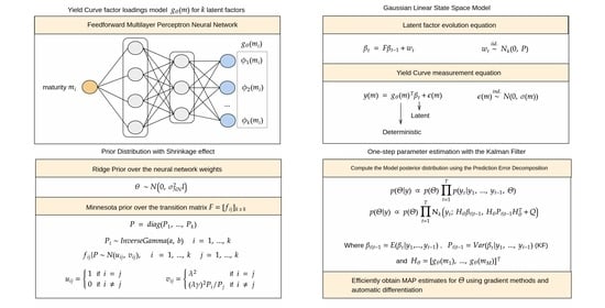
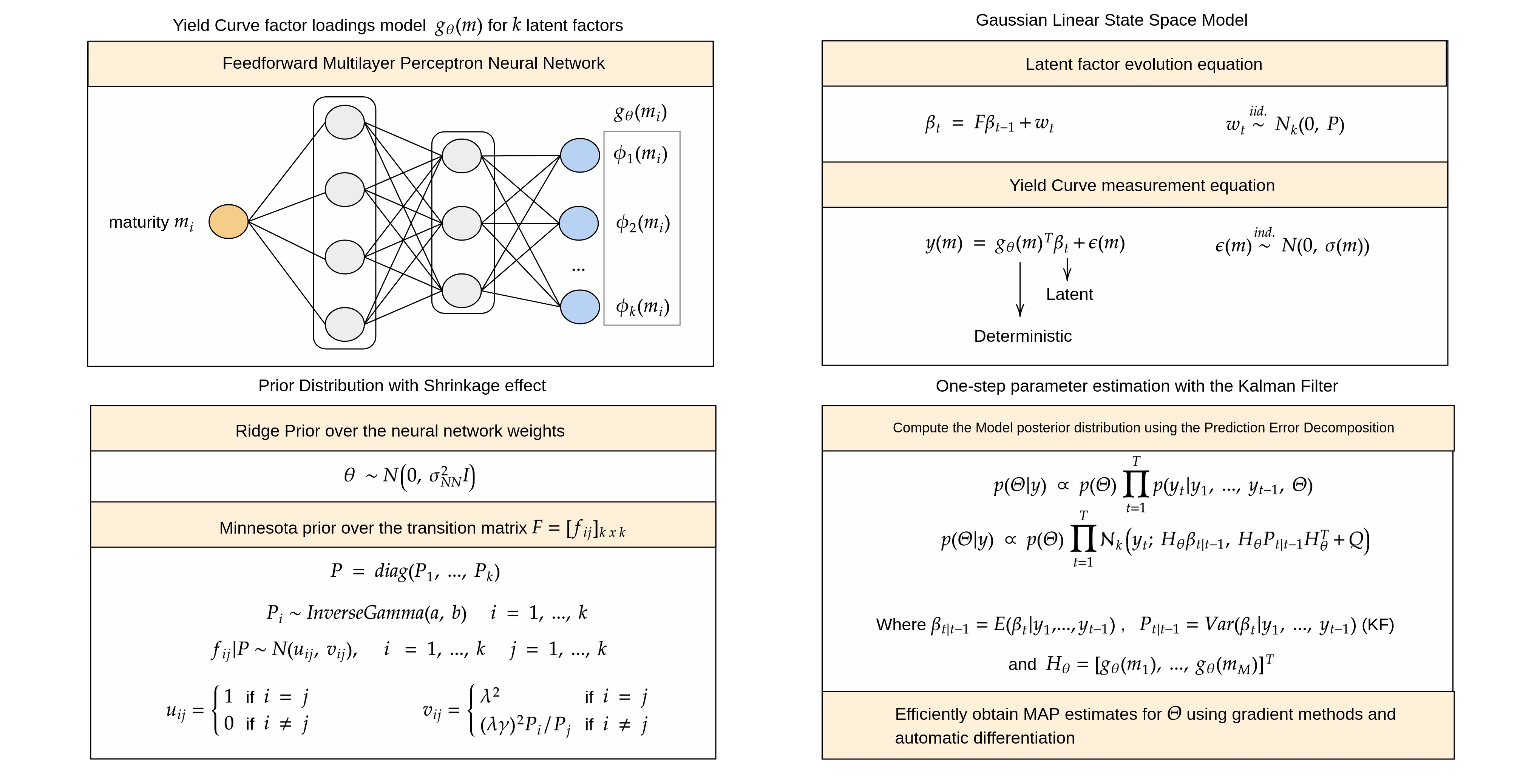
In this paper, we propose augmenting the Gaussian linear state-space model structure of yield curve factor models with a neural network that generates parameterized smooth factor loading functions, which can be jointly estimated with the transition parameters in one step. To help ensure that the generated yield curve factor loadings have good properties (such as smoothness) and to avoid the problem of overfitting in the temporal component of the model, we specify prior distributions for the model parameters that reflect these premises.
Among all of the works reviewed, our approach bears the greatest resemblance to the model proposed by Hays et al. (2012), although we highlight some key differences. Natural cubic splines depend on the number and position of knots, which need to be set beforehand, whereas neural networks do not have such a requirement. In practice, selecting the number and position of knots can be a difficult task, which can significantly impact the resulting curve. Secondly, due to computational constraints, Hays et al. (2012) estimate each factor loading function sequentially. In this work, we remove this restriction and estimate all factor loading functions simultaneously. Finally, we also investigate the impact of prior distributions with a regularization effect on both state and space parameters of yield curve forecasting models.
In an empirical evaluation conducted on 14 years of Brazilian yield curve data, we find that the proposed technique achieves better out-of-sample forecasting performance than traditional methods while still maintaining the advantageous properties of classic yield curve models. Given its similarity to long-established factor-based models, we highlight that the proposed technique can also be adapted to include a wide range of extensions proposed in the yield curve forecasting literature in the last decades, which may constitute an interesting topic for future studies.
The rest of this paper is organized as follows. We briefly review the dynamic Nelson and Siegel model family and parameter estimation approaches in Section 2. In Section 3, we introduce the neural network augmented state-space model. In Section 4 and Section 5, we evaluate the proposed model’s performance and present our concluding remarks.
2. Dynamic Nelson and Siegel Model and Extensions
2.1. The Dynamic Nelson and Siegel Model
In their seminal work, Nelson and Siegel (1987) propose a parsimonious three-factor yield curve model that can represent a variety of common yield curve shapes with precision. The Nelson and Siegel model (written using Diebold and Li (2006) parameterization) for the yield curve y evaluated at maturity m is given by
where m is the yield maturity; , , and are the yield curve factors; is an exponential decay parameter; and is an uncorrelated error term.
By individually estimating the parameters of the Nelson and Siegel model, any given yield curve y can be succinctly represented in four-dimensional space constructed using the obtained yield curve factors and exponential decay term, effectively functioning as a dimensionality reduction technique.
An advantage of the Nelson and Siegel yield curve formulation is the existence of economic interpretations of the model factors. The intercept parameter can be regarded as a long-term factor, given that asymptotically approaches as m increases. The factor can be interpreted as a short-term factor, since the factor loading function is a strictly decreasing function starting at 1 and decreasing toward 0. Lastly, the third factor is interpreted as a medium-term factor due to the fact that the loading function starts at 0, reaches a positive peak, and then decays toward 0.
The parameter affects the rate of decay of both short- and medium-term factor loadings as well as the location of the peak in the medium-term loading. Nelson and Siegel (1987) recommend treating the exponential decay parameter as fixed, allowing the factors to be estimated through ordinary least squares (OLS), significantly simplifying the estimation procedure.
In order to adapt the Nelson and Siegel decomposition of the term structure to the forecasting setting, Diebold and Li (2006) models the evolution of the latent yield curve factors as an autoregressive process:
where is a vector of factors at time t, F and P are 3 × 3 matrices, and P is a positive semi-definite matrix. For a fixed set of maturities , the above expression can be further simplified to
where , Q is a diagonal positive semi-definite matrix, and the factor loading matrix is given by
The estimation method of Diebold and Li (2006), which is often referred to as the two-step dynamic Nelson and Siegel model, involves first extracting the Nelson and Siegel factors independently for each yield curve and then fitting the autoregressive model with the factors extracted in the first step. In order to increase the numerical stability and computational efficiency of the first step, the exponential decay parameter is treated as fixed, allowing the estimation of the Nelson and Siegel factors through ordinary least squares (OLS) estimation, as noted before. Diebold and Li (2006) further suggest fixing the exponential decay parameter as the value that maximizes the medium-term loading function when evaluated at the average sample maturity . Alternatively, a grid search procedure can also be used to select , as suggested by Nelson and Siegel (1987).
More generally, the dynamic Nelson and Siegel model is a particular case of the Gaussian linear state-space model (often also referred in this context to as the dynamic Gaussian factor model) with measurement Equation (4) and state transition Equation (3), as shown in Diebold et al. (2006). Therefore, the parameters of the state transition and measurement equations can be jointly estimated using the prediction error decomposition to compute the model likelihood. This general estimation procedure is described in more detail in the next section.
2.2. The Dynamic Nelson, Siegel, and Svensson Model
In order to increase the model flexibility, Svensson (1994) includes a fourth factor in the Nelson and Siegel decomposition:
where , , , , and are defined as before, and is a new factor with the exponential decay parameter .
Svensson (1994) notes that the inclusion of another medium-term factor () and a second exponential decay parameter significantly increases the flexibility of the model to fit more yield curve shapes. Due to its direct similarities to the Nelson and Siegel model, a dynamic version of the Svensson model can be easily constructed following the same steps described in the previous section.
3. Neural Network Augmented State-Space Model
3.1. Model Definition
A natural extension of the discussed modeling approaches is to try to learn the interest rate term structure decomposition directly from data. For a model with k factors, an intuitive approach is to estimate the entire measurement matrix H with M × k free parameters simultaneously with the rest of the Gaussian linear state-space model parameters. However, this approach suffers from two main disadvantages: forecasts cannot be computed for unobserved maturities without requiring an interpolation or extrapolation procedure, and, most importantly, the model does not induce similarity among interest rates with similar maturities, which is a fundamental property of yield curves. We refer to the latter as the stability property (or smoothness) of the factor loadings.
To tackle both of these issues while still preserving model flexibility, we propose the following yield curve factor model for k arbitrary factors:
where m is the yield maturity, are the k yield curve factors at time t, and is a feedforward neural network (with parameter vector ) that maps a yield maturity m to the corresponding vector of factor loadings:
The structure of the neural network guarantees continuous and differentiable factor loadings, allowing the evaluation of the yield curve at any given maturity, as in the dynamic Nelson and Siegel model. Continuous factor decompositions can be learned from data by estimating the parameter vector from the neural network , but since neural networks are powerful general function approximators, we highlight the importance of restricting the network weights in order to produce stable factor loadings. A restriction in the form of a prior distribution over the neural network weights is described in the next section.
In order to simplify the model interpretation, we set and evaluate only at a constant vector of maturities , producing the following compact measurement equation:
where . Conditional on , the linear form of the model is preserved, and therefore, the Kalman filter (Kalman 1960) can be used to compute the conditional distribution of given the last observations. This property allows the direct computation of the posterior density function of the model, which is given by
where is the Gaussian probability density function. The terms and are obtained directly from the Kalman recurrence equations. This procedure is also known as the prediction error decomposition.
Point estimates for the model parameters can be obtained by maximizing the posterior density function with gradient-based optimization methods. The gradient can be efficiently computed for any given differentiable neural network architecture using automatic differentiation algorithms (Rall 1986; Wengert 1964), which can outperform numerical differentiation algorithms, especially in high-dimensional parameter spaces. The cost of computing the Kalman filter in each evaluation of the posterior density function can also be reduced using the parallel algorithm proposed by Särkkä and García-Fernández (2019), which achieves logarithmic span-complexity when multiple processing units are available.
Despite the similarities to Gaussian linear state-space models, performing fully Bayesian inference that relies on sampling methods for the model parameters can be challenging, since neural network models are usually overparameterized and suffer from low parameter identifiability. In recent years, there has been an increasing amount of literature on approximate inference methods for quantifying uncertainty in Bayesian neural networks (see Filos et al. 2019 for a benchmark and discussion of current approaches), but it is not in the scope of this work to provide accurate probabilistic forecasts. Nevertheless, we note that this limitation may pose a challenge for practitioners interested in yield curve forecasting from a risk management perspective.
3.2. Specification of Prior Distribution
Neural networks are known to typically require a large number of parameters to model complex functions and to be usually prone to overfitting in the absence of large datasets or regularization mechanisms (Barron 1991). As (Neal 1992; MacKay 1992) show, the Bayesian framework can be successfully applied to neural networks, providing a variety of theoretically solid regularization techniques based on the choice of the prior distribution defined over the neural network weights. One common choice of the prior distribution is the zero-centered uncorrelated normal distribution:
This prior distribution induces an weight penalty (also known as the ridge penalty Hoerl and Kennard (1970)) on the posterior distribution density function. The amount of shrinkage is controlled by the hyperparameter , where smaller values of induce larger penalties.
Another well-studied use of Bayesian shrinkage priors is in vector autoregressive (VAR) models, where the number of parameters can also be excessive in high dimensions. One commonly chosen prior distribution is the “Minnesota prior” (Litterman 1986), which assigns a normal distribution centered around a random walk to the VAR coefficients. This hypothesis is especially useful for yield curve forecasting, since the random walk model is usually a tough benchmark to beat, especially over short horizons (see Diebold and Li 2006; Ang and Piazzesi 2003, for instance).
Instead of the empirical Bayes approach described by Litterman (1986), we use a common variation of the Minnesota prior based on the normal and inverse gamma conjugacy:
where the state equation noise term covariance matrix P is a diagonal matrix of components , is a term in the transition matrix F, and the quantities and are defined as
The hyperparameter controls the strength of the support for the random walk hypothesis, while controls the importance of the relationship between different factors relative to .
In the next section, we perform an empirical comparison of the out-of-sample forecasting performance between the proposed model and approaches based on the dynamic Nelson and Siegel model. At the end of Section 4, the impact of the prior distribution hyperparameters is also briefly analyzed.
4. Empirical Evaluation
4.1. Experimental Setup
In order to empirically assess the forecasting performance of the proposed technique, we use the Brazilian yield curve constructed by the B3 Brazilian Stock Exchange using future interbank deposit rates, as commonly used in the Brazilian term structure modeling literature (see Caldeira et al. 2010; Vicente and Tabak 2008; Cajueiro et al. 2009, for instance). We consider 15 years of Brazilian yield curve data from August 2003 to August 2018 using the 11 maturities at 1, 2, 3, 6, 12, 24, 36, 48, 60, 72, and 84 business months. The missing yield curve vertices are interpolated using the “flat-forward” method (Maltz 2002).
For this experiment, we benchmark out-of-sample forecasts obtained with the proposed neural network augmented state-space model (NNSS) against the following classical modeling approaches: the random walk model (RW), the dynamic Nelson and Siegel model (DNS), and the dynamic Nelson, Siegel, and Svensson model (DSV). The DNS and DSV models are both evaluated using the two-step and one-step parameter estimation approaches. In order to assess whether the inclusion of the neural network component is beneficial to the proposed model, we also benchmark a complete Gaussian linear state-space model (GLSS), where the entire measurement matrix H is estimated directly with the remaining parameters. To verify whether four-factor models are sufficient, we test both NNSS and GLSS models using four and five latent factors.
In the two-step estimation approach for the DNS and DSV models, following the method described by Nelson and Siegel (1987), a grid search procedure is used to choose the exponential decay parameters that minimize the total sum of squares of the real yield curve and the curve reconstructed from the decomposition factors . The obtained values are also used in the respective one-step models.
To increase numerical stability and accelerate convergence, we initialize the one-step DNS and DSV with the estimates obtained in the two-step approach. For the same purpose, we also initialize the measurement matrix H of the GLSS model with the factor loading matrix used in the DSV model. Similarly, the neural network parameter vector of the NNSS is also initialized with a solution that closely reproduces (in the squared error sense) the DSV factor loadings. This is carried out by pre-training the neural network with that objective.
In all NNSS models, we use a neural network with two hidden layers, both with 300 hidden units intercalated with hyperbolic tangent activation functions, which are smooth and have good convergence properties (LeCun et al. 2012). To help interpret the model factors and obtain factor loadings that are similar to those of the Nelson and Siegel model, we use a sigmoid activation function in the last layer of the neural network, which produces factor loading functions bounded in the interval.
The models based on the one-step approach are estimated using gradient-based optimization methods with the Pytorch deep learning library (Paszke et al. 2019) and the parallel-scan Kalman filter algorithm (Särkkä and García-Fernández 2019) implemented in the Pyro probabilistic programming library (Bingham et al. 2019) in the Python programming language.
The prior distribution hyperparameters of the NNSS model are chosen based on the results obtained using the one-step DSV model and with the aid of simulation procedures. In this experiment, we use weakly informative prior distributions in order to assess the model behavior in the absence of strong external influences. A more comprehensive analysis of the impact of the prior distribution on model performance is presented at the end of the results section.
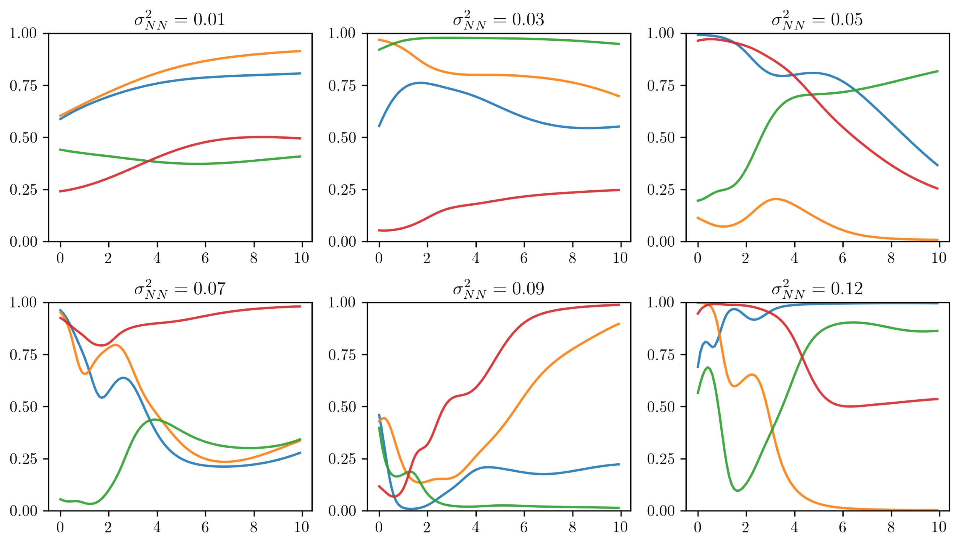
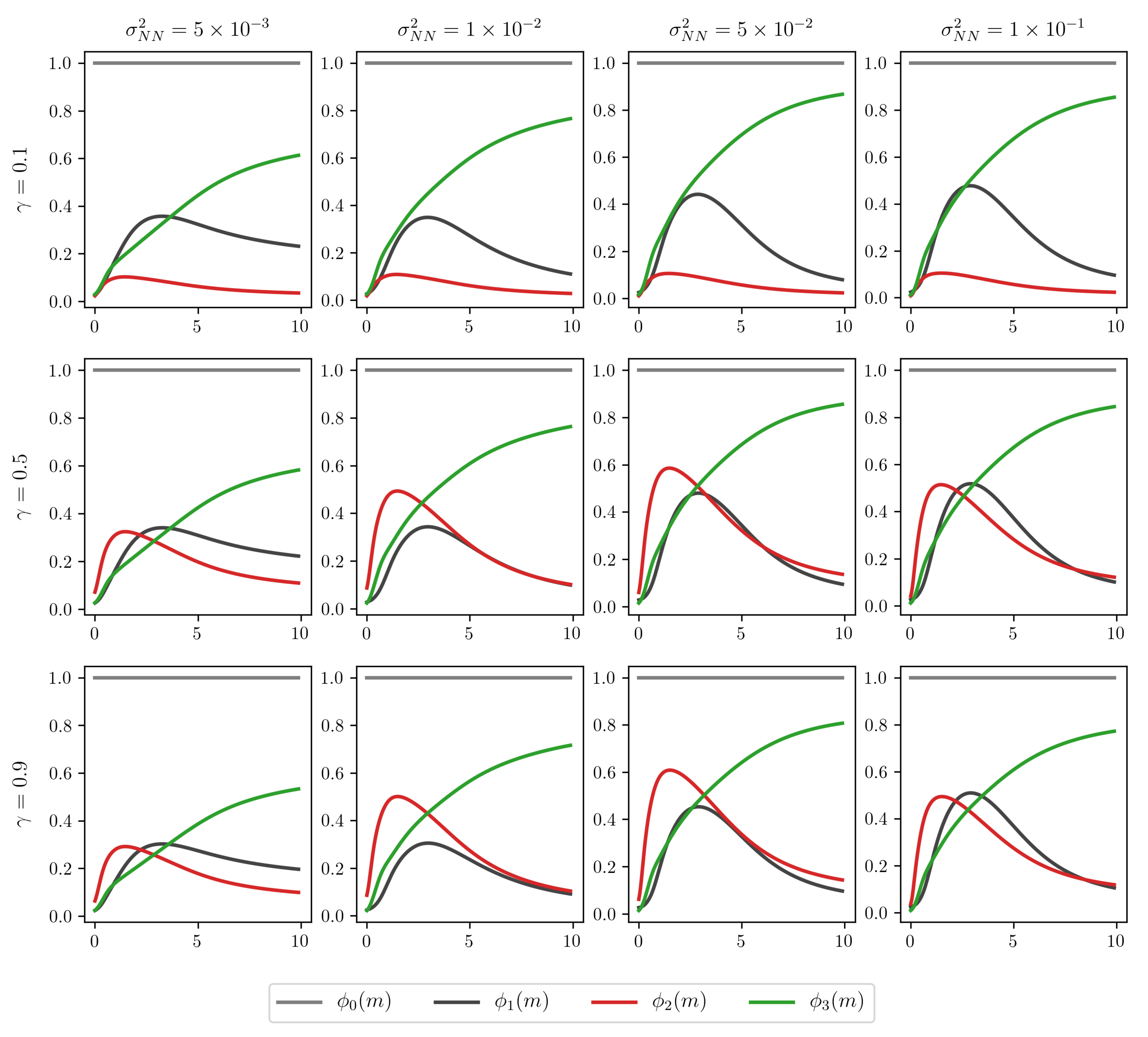
For the hyperparameters of the inverse gamma distribution, we select such that the resulting prior is weakly informative, and the mode of the distribution is close to the estimated state transition variances of the DSV model. The remaining hyperparameters of the Minnesota prior are chosen in a qualitative fashion by simulating the resulting prior transition matrices and determining whether the samples generally match our expected results while still preserving variability. Analogously, the same process is used to choose the prior variance of neural network weights (Figure 1).
4.2. Forecast Evaluation
Given the computational complexity of the NNSS model, we evaluate all of the described modeling approaches using only the first 12 years of data to estimate model parameters once and the remaining 3 years to evaluate the out-of-sample forecasts for 1 week, 1 month, 3 months, and 6 months ahead. For the models based on the two-step approach, the h-step ahead forecasts at time t are calculated by evolving the extracted factors available at t to step , which is carried out using the estimated VAR model. Then, the resulting prediction is converted to yield curve format using the decomposition equation.
For the models based on the one-step estimation approach, the procedure is similar, but it requires the extra step of updating the Kalman filter at the end of each iteration. The complete procedure is described below for each timestep t:
- Obtain the forecast of the yield curve factors from t using the filtered factors and the estimated transition matrix ;
- Convert the forecasted factors using the estimated measurement matrix to obtain the prediction of the complete yield curve from t to :
- Update the Kalman filter recurrence equations using the next observation to obtain .
Then, the forecasts are evaluated using the root-mean-square error metric (RMSE), which is calculated for each considered maturity m and horizon h as:
where denotes the index of the first out-of-sample observation, is the forecast from t to of the yield curve for maturity m, and T is the total number of observations in the dataset.
4.3. Results
Table 1, Table 2, Table 3 and Table 4 report the RMSE of the out-of-sample forecasts of the nine considered models for the four forecast horizons. For each model, we report error metrics for each of the 11 considered maturities as well as the average and standard deviation.
In the 1-week ahead forecasts (Table 1), all models except for the 5-GLSS model and the dynamic Nelson and Siegel model achieved better overall scores than the random walk (RW) method, which is typically a tough benchmark to beat over short horizons. The five-factor NNSS model achieved a slightly lower average RMSE score, which is followed closely by the four-factor NNSS model.
In the 1-month ahead forecast (Table 2), the NNSS models still achieved the lowest average RMSE, but we note that the DSV models performed better than the rest of the contenders. Overall, among all of the models, the DSV models had the best performance on short- and medium-term maturities, while the NNSS models had the best performance on longer maturities.
A similar pattern can be identified in the 3-month ahead forecast results, although the performance gap between the NNSS models and the other candidates becomes more noticeable. Surprisingly, for the DSV model, the two-step approach has perceptibly lower RMSE scores than the one-step version. We also note that the performance of the GLSS models decreased significantly, remaining only above that of the DNS models and the random walk method.
In the longest considered forecast horizon of 6 months, the relative performance of the NNSS models with respect to the other candidates was greatly improved, especially for the five-factor model. We also observe that the two-step DSV model and the 5-GLSS model achieved good performance.
The estimated yield curve factor loadings of the DNS, DSV, GLSS, and NNSS models are plotted in Figure 2. As expected, the factor loadings of the GLSS models present non-smooth behavior, especially the four-factor GLSS model. Despite being initialized with the factor loadings of the DSV model, the estimated loadings of the GLSS models seem to have lost the original asymptotic behavior of the Nelson and Siegel decomposition, which can make the process of extrapolating the factor loadings outside of the original range of maturities difficult and unreliable in a real-world setting.
Unlike the GLSS models, the factor loadings of both four- and five-factor NNSS exhibit a smooth and stable pattern. We also note that, as in the Nelson and Siegel decomposition, the obtained factor loading functions display asymptotic stable behavior, which is a well-known stylized fact about yield curves. We attribute this property of the NNSS model to the choice of the sigmoid activation function in the output layer of the neural network .
In some ways, the interpretation of some of the yield curve factors from the 4-NNSS model is similar to that of the Nelson, Siegel, and Svensson model. For instance, factors 1 and 2 can be interpreted as two medium-term factors with peaks around the 1.5- and 3-year maturities, although the first factor loading exhibits a steeper growth and decay rate as well as a slight bump around the shorter maturities. Another notable difference between the 4-NNSS and DSV factors can be seen in the third loading function, which resembles a mirrored version of the exponential decay pattern of the first Nelson and Siegel loading. Therefore, the intercept term in the 4-NNSS model can be interpreted as a short-term factor.
In the five-factor version of the NNSS model, the interpretation of the factors becomes slightly convoluted, but it is possible to identify a short-term factor (factor 1) and three different kinds of medium- and long-term factors (factors 2, 3, and 4). Similar to the first loading of the 4-NNSS model, we also observe a bump in the fourth loading of the 5-NNSS model located at the short end of the yield curve, which indicates that this factor also has some influence on shorter maturities.
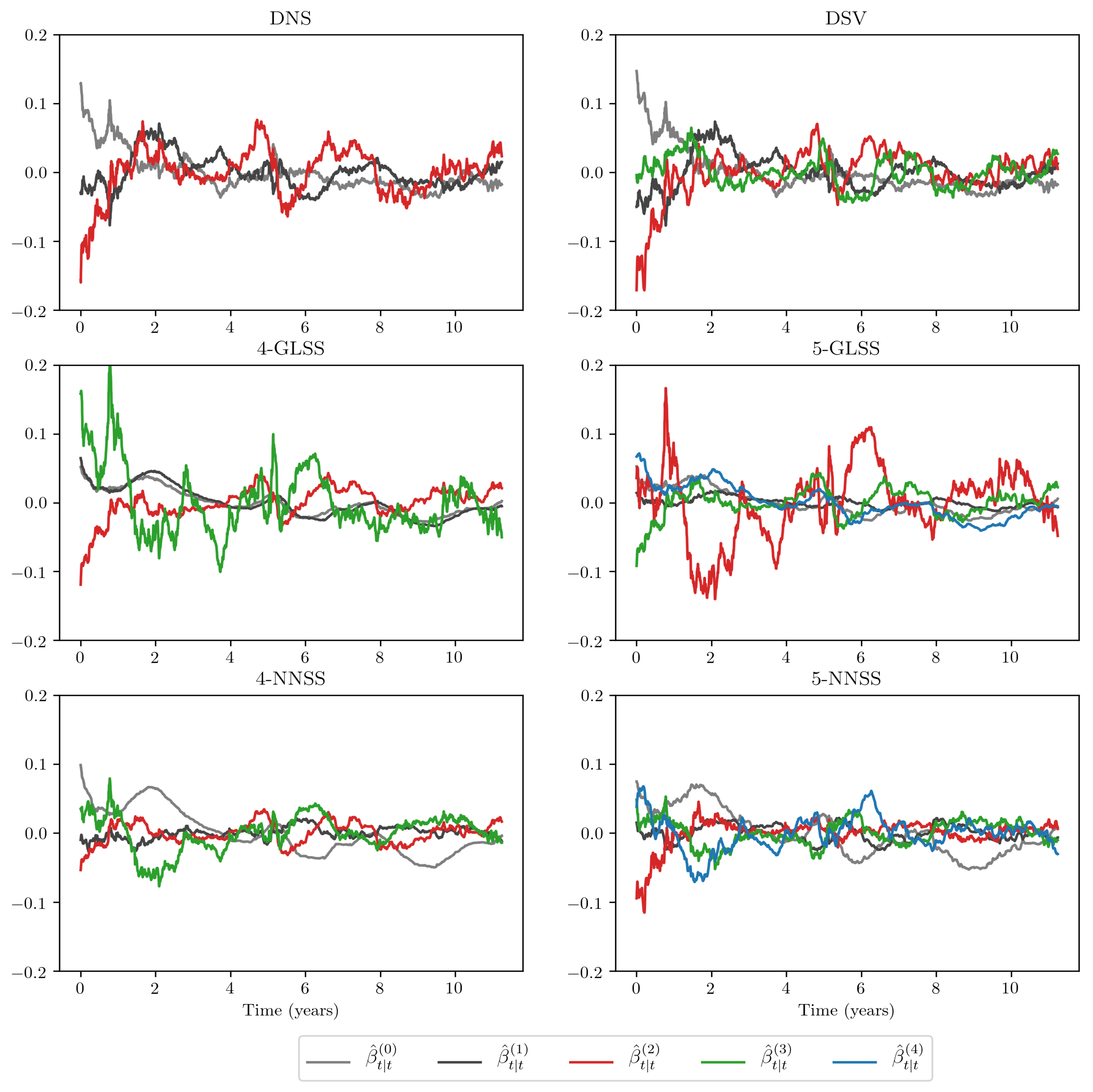
Figure 3 presents the time-series of the filtered yield curve factors for each considered model. The extracted factors of the 4-GLSS and 5-GLSS models exhibit a great amount of variability, especially in the second and third factors. Among all of the evaluated decompositions, the yield curve factors from the NNSS models are the most stable, which indicates that the learned decompositions are useful for the forecasting task.
4.4. Impact Analysis of the Prior Distribution Hyperparameters
In order to empirically assess the impact of the specified prior distribution in the proposed model, we repeat the forecast experiment described in the previous section for the 4-NNSS model with a variable set of hyperparameters. The four-factor version of the NNSS model was used due to the faster convergence of the model parameters and easier factor loading interpretation.
The experimental results reported in Table 5 verify that the Minnesota prior distribution significantly impacted the overall forecasting performance of the model, especially over longer horizons. The forecast accuracy dropped significantly under the strongest penalty tested (), although a medium penalty value () produced better results than the weakly informative prior used in the previous experiment ().
The neural network shrinkage prior slightly affected the overall forecast performance; in the models estimated with , a stronger penalty (lower value for ) produced a small but consistent gain in forecast performance. The factor loading plot for each tested model is included in Appendix A.
5. Conclusions
In this paper, we proposed a yield curve forecasting model that learns continuous and smooth decompositions directly from data using a neural network. We showed how the neural network can be integrated into a Gaussian linear state-space model and presented a joint estimation procedure to obtain maximum a posteriori (MAP) estimates for decomposition and autoregressive parameters.
In the empirical evaluation, we obtained better overall out-of-sample forecast performance than traditional approaches on 14 years of Brazilian yield curve data, especially for longer maturities and forecast horizons. By analyzing the generated decompositions, we found that the model was able to reproduce the advantageous properties of traditional yield curve models, such as the smoothness, asymptotic stability, and economic interpretability of the factor loadings, and that the learned decompositions produced yield curve factors that were more stable and easier to forecast than those obtained with traditional approaches.
Finally, we analyzed the role of the prior distribution hyperparameters in the out-of-sample forecasting performance and found that the shrinkage effect on the model parameters can significantly influence the quality of the produced forecasts, especially over longer time horizons. We found that stronger penalties for the weights in the neural network () and medium-level penalties in the state equation parameters () resulted in the best overall prediction performance in the experiments performed.
Given the direct similarities, we note that a wide range of extensions developed for the dynamic Nelson and Siegel model can also be adapted to the technique proposed in this paper, such as the inclusion of macroeconomic variables in the state equation (Diebold et al. 2006) and multicountry modeling (Diebold et al. 2008), which may be interesting topics for future research.
Another possible line of research concerns the optimization method used to obtain point estimates for the model parameters, since pure gradient-based optimization methods in state-space models can be unstable and require the careful selection of step sizes. As commonly used in the dynamic factor modeling literature, the Expectation-Maximization (EM) algorithm can be a robust alternative that usually approaches an optimal neighborhood very quickly, but it requires many iterations to reach full convergence. As noted by Watson and Engle (1983), the EM algorithm can be used to quickly provide good starting points to a gradient-based optimization algorithm, combining the best parts of both approaches. For the method proposed in this paper, the maximization step of the EM algorithm would also require the internal use of iterative methods, given the non-linear nature of the neural network component, but it could effectively increase the robustness of the overall optimization procedure.
The computer code used in this work, written in the Python programming language, is available in the Supplementary Materials.
Supplementary Materials
The following supporting information can be downloaded at: https://0-www-mdpi-com.brum.beds.ac.uk/article/10.3390/econometrics10020015/s1.
Author Contributions
Conceptualization, P.C.K.; methodology, P.C.K. and H.H.T.; software, P.C.K.; validation, H.H.T., A.T.T. and J.M.S.; formal analysis, P.C.K., H.H.T. and J.M.S.; investigation, A.T.T.; resources, J.M.S.; data curation, P.C.K. and A.T.T.; writing—original draft preparation, P.C.K.; writing—review and editing, H.H.T., A.T.T. and J.M.S.; visualization, P.C.K.; supervision, H.H.T. and J.M.S.; project administration, J.M.S. All authors have read and agreed to the published version of the manuscript.
Funding
This research received no external funding.
Institutional Review Board Statement
Not applicable.
Data Availability Statement
Restrictions apply to the availability of these data. Data was obtained from the B3 Brazillian Stock Exchange website (https://www.b3.com.br) accessed on 24 February 2019.
Conflicts of Interest
The authors declare no conflict of interest.
Appendix A
Figure A1.
Factor loading functions of the 4-NNSS model up to 10 years of maturity for each combination of the prior hyperparameters and while keeping and fixed.
Figure A1.
Factor loading functions of the 4-NNSS model up to 10 years of maturity for each combination of the prior hyperparameters and while keeping and fixed.

References
- Ang, Andrew, and Monika Piazzesi. 2003. A no-arbitrage vector autoregression of term structure dynamics with macroeconomic and latent variables. Journal of Monetary Economics 50: 745–87. [Google Scholar] [CrossRef]
- Barron, Andrew R. 1991. Complexity regularization with application to artificial neural networks. In Nonparametric Functional Estimation and Related Topics. Dordrecht: Springer, pp. 561–76. [Google Scholar]
- Bingham, Eli, Jonathan P. Chen, Martin Jankowiak, Fritz Obermeyer, Neeraj Pradhan, Theofanis Karaletsos, Rohit Singh, Paul Szerlip, Paul Horsfall, and Noah D. Goodman. 2019. Pyro: Deep universal probabilistic programming. The Journal of Machine Learning Research 20: 973–78. [Google Scholar]
- Bowsher, Clive G., and Roland Meeks. 2008. The dynamics of economic functions: Modeling and forecasting the yield curve. Journal of the American Statistical Association 103: 1419–37. [Google Scholar] [CrossRef] [Green Version]
- Cajueiro, Daniel O., Jose A. Divino, and Benjamin M. Tabak. 2009. Forecasting the yield curve for Brazil. Central Bank of Brazil Working Paper Series 197: 1–30. [Google Scholar]
- Caldeira, Joao, Guilherme V. Moura, and Marcelo Savino Portugal. 2010. Efficient yield curve estimation and forecasting in Brazil. Revista Economia 11: 27–51. [Google Scholar]
- Cox, John C., Jonathan E. Ingersoll Jr., and Stephen A. Ross. 2005. A theory of the term structure of interest rates. In Theory of Valuation. Singapore: World Scientific, pp. 129–64. [Google Scholar]
- Diebold, Francis X., and Canlin Li. 2006. Forecasting the term structure of government bond yields. Journal of Econometrics 130: 337–64. [Google Scholar] [CrossRef] [Green Version]
- Diebold, Francis X., Glenn D. Rudebusch, and S. Boragan Aruoba. 2006. The macroeconomy and the yield curve: A dynamic latent factor approach. Journal of Econometrics 131: 309–38. [Google Scholar] [CrossRef] [Green Version]
- Diebold, Francis X., Canlin Li, and Vivian Z. Yue. 2008. Global yield curve dynamics and interactions: A dynamic Nelson–Siegel approach. Journal of Econometrics 146: 351–63. [Google Scholar] [CrossRef] [Green Version]
- Duffie, Darrell, and Rui Kan. 1996. A yield-factor model of interest rates. Mathematical Finance 6: 379–406. [Google Scholar] [CrossRef] [Green Version]
- Faria, Adriano, and Caio Almeida. 2018. A hybrid spline-based parametric model for the yield curve. Journal of Economic Dynamics and Control 86: 72–94. [Google Scholar] [CrossRef]
- Filos, Angelos, Sebastian Farquhar, Aidan N. Gomez, Tim G. J. Rudner, Zachary Kenton, Lewis Smith, Milad Alizadeh, Arnoud de Kroon, and Yarin Gal. 2019. A Systematic Comparison of Bayesian Deep Learning Robustness in Diabetic Retinopathy Tasks. arXiv arXiv:1912.10481. [Google Scholar]
- Hays, Spencer, Haipeng Shen, and Jianhua Z. Huang. 2012. Functional dynamic factor models with application to yield curve forecasting. The Annals of Applied Statistics 6: 870–94. [Google Scholar] [CrossRef]
- Heath, David, Robert Jarrow, and Andrew Morton. 1992. Bond pricing and the term structure of interest rates: A new methodology for contingent claims valuation. Econometrica: Journal of the Econometric Society 60: 77–105. [Google Scholar] [CrossRef]
- Hoerl, Arthur E., and Robert W. Kennard. 1970. Ridge regression: Applications to nonorthogonal problems. Technometrics 12: 69–82. [Google Scholar] [CrossRef]
- Hull, John, and Alan White. 1990. Pricing interest-rate-derivative securities. The Review of Financial Studies 3: 573–92. [Google Scholar] [CrossRef]
- Kalman, Rudolph Emil. 1960. A New Approach to Linear Filtering and Prediction Problems. Transactions of the ASME–Journal of Basic Engineering 82: 35–45. [Google Scholar] [CrossRef] [Green Version]
- LeCun, Yann A., Léon Bottou, Genevieve B. Orr, and Klaus-Robert Müller. 2012. Efficient backprop. In Neural Networks: Tricks of the Trade. Berlin/Heidelberg: Springer, pp. 9–48. [Google Scholar]
- Litterman, Robert B. 1986. Forecasting with Bayesian vector autoregressions—Five years of experience. Journal of Business & Economic Statistics 4: 25–38. [Google Scholar]
- MacKay, David J. C. 1992. A practical Bayesian framework for backpropagation networks. Neural Computation 4: 448–72. [Google Scholar] [CrossRef]
- Maltz, Allan. 2002. Estimation of zero coupon curves in Datametrics. RiskMetrics Journal 3: 27–39. [Google Scholar]
- Mineo, Eduardo, Airlane Pereira Alencar, Marcelo Moura, and Antonio Elias Fabris. 2020. Forecasting the Term Structure of Interest Rates with Dynamic Constrained Smoothing B-Splines. Journal of Risk and Financial Management 13: 65. [Google Scholar] [CrossRef] [Green Version]
- Neal, Radford M. 1992. Bayesian Training of Backpropagation Networks by the Hybrid Monte Carlo Method. Technical Report, Citeseer. Toronto: Department of Computer Science, University of Toronto. [Google Scholar]
- Nelson, Charles R., and Andrew F. Siegel. 1987. Parsimonious modeling of yield curves. Journal of Business 60: 473–89. [Google Scholar] [CrossRef]
- Paszke, Adam, Sam Gross, Francisco Massa, Adam Lerer, James Bradbury, Gregory Chanan, Trevor Killeen, Zeming Lin, Natalia Gimelshein, Luca Antiga, and et al. 2019. Pytorch: An imperative style, high-performance deep learning library. Advances in Neural Information Processing Systems 32: 8026–37. [Google Scholar]
- Rall, Louis B. 1986. The Arithmetic of Differentiation. Mathematics Magazine 59: 275–82. [Google Scholar] [CrossRef]
- Särkkä, Simo, and Ángel F. García-Fernández. 2019. Temporal parallelization of bayesian filters and smoothers. arXiv arXiv:1905.13002. [Google Scholar]
- Svensson, Lars E. O. 1994. Estimating and Interpreting forward Interest Rates: Sweden 1992–1994. Technical Report. Cambridge, MA: National Bureau of Economic Research. [Google Scholar]
- Takada, Hellinton H., and Julio M. Stern. 2015. Non-negative matrix factorization and term structure of interest rates. AIP Conference Proceedings American Institute of Physics 1641: 369–77. [Google Scholar]
- Vasicek, Oldrich. 1977. An equilibrium characterization of the term structure. Journal of Financial Economics 5: 177–88. [Google Scholar] [CrossRef]
- Vicente, José, and Benjamin M. Tabak. 2008. Forecasting bond yields in the Brazilian fixed income market. International Journal of Forecasting 24: 490–97. [Google Scholar] [CrossRef]
- Watson, Mark W., and Robert F. Engle. 1983. Alternative algorithms for the estimation of dynamic factor, mimic and varying coefficient regression models. Journal of Econometrics 23: 385–400. [Google Scholar] [CrossRef] [Green Version]
- Wengert, Robert Edwin. 1964. A Simple Automatic Derivative Evaluation Program. Communications of the ACM 7: 463–64. [Google Scholar] [CrossRef]
Figure 1.
Samples of the factor loading functions under the prior distribution for six different values of the hyperparameter .
Figure 1.
Samples of the factor loading functions under the prior distribution for six different values of the hyperparameter .

Figure 2.
Estimated factor loadings of the DNS and DSV models, 4- and 5-factor GLSS models, and 4- and 5-factor NNSS models. The factor loadings for the GLSS models are linearly interpolated within the range of the 11 maturities considered in the dataset; factor loadings for maturities outside of this range are not extrapolated.

Figure 3.
Filtered yield curve factors from the dataset for the one-step DNS, one-step DSV, 4- and 5-factor GLSS, and 4- and 5-factor NNSS.
Figure 3.
Filtered yield curve factors from the dataset for the one-step DNS, one-step DSV, 4- and 5-factor GLSS, and 4- and 5-factor NNSS.


Table 1.
Out-of-sample RMSE × of 1-week ahead forecasts (lowest scores in bold).
| Model | Maturity (Business Months) | Avg. | Std. | ||||||||||
|---|---|---|---|---|---|---|---|---|---|---|---|---|---|
| 1 | 2 | 3 | 6 | 12 | 24 | 36 | 48 | 60 | 72 | 84 | |||
| RW | 0.95 | 0.95 | 1.07 | 1.47 | 1.99 | 2.66 | 2.90 | 2.98 | 3.02 | 3.03 | 3.03 | 2.19 | 0.87 |
| 2-step DNS | 1.02 | 0.79 | 1.14 | 2.15 | 2.54 | 2.66 | 2.99 | 3.03 | 3.00 | 3.15 | 3.34 | 2.34 | 0.89 |
| 1-step DNS | 1.10 | 0.81 | 1.17 | 2.20 | 2.53 | 2.80 | 2.95 | 2.94 | 2.95 | 3.05 | 3.20 | 2.34 | 0.84 |
| 2-step DSV | 0.77 | 0.79 | 1.05 | 1.46 | 2.16 | 2.68 | 2.90 | 3.01 | 2.98 | 3.04 | 3.15 | 2.18 | 0.93 |
| 1-step DSV | 0.75 | 0.78 | 0.98 | 1.35 | 2.18 | 2.81 | 2.81 | 2.90 | 2.95 | 3.01 | 3.12 | 2.15 | 0.93 |
| 4-GLSS | 0.71 | 0.75 | 0.97 | 1.51 | 2.16 | 2.79 | 2.81 | 2.89 | 2.96 | 3.01 | 3.08 | 2.15 | 0.93 |
| 5-GLSS | 0.69 | 0.89 | 1.28 | 1.89 | 2.10 | 2.60 | 2.87 | 3.06 | 3.10 | 3.02 | 3.01 | 2.23 | 0.87 |
| 4-NNSS | 0.75 | 0.73 | 0.89 | 1.36 | 2.08 | 2.80 | 2.81 | 2.90 | 2.96 | 3.00 | 3.05 | 2.12 | 0.94 |
| 5-NNSS | 0.66 | 0.72 | 0.89 | 1.37 | 2.07 | 2.65 | 2.85 | 2.96 | 3.00 | 2.98 | 2.96 | 2.10 | 0.95 |
Table 2.
Out-of-sample RMSE × of 1-month ahead forecasts (lowest scores in bold).
| Model | Maturity (Business Months) | Avg. | Std. | ||||||||||
|---|---|---|---|---|---|---|---|---|---|---|---|---|---|
| 1 | 2 | 3 | 6 | 12 | 24 | 36 | 48 | 60 | 72 | 84 | |||
| RW | 3.27 | 3.24 | 3.34 | 3.75 | 4.40 | 5.34 | 5.76 | 5.91 | 5.98 | 6.00 | 6.00 | 4.82 | 1.16 |
| 2-step DNS | 1.57 | 1.98 | 2.57 | 3.86 | 4.72 | 5.09 | 5.60 | 5.92 | 6.02 | 6.25 | 6.47 | 4.55 | 1.70 |
| 1-step DNS | 1.58 | 1.94 | 2.51 | 3.75 | 4.65 | 5.19 | 5.36 | 5.56 | 5.73 | 5.88 | 6.04 | 4.38 | 1.58 |
| 2-step DSV | 1.31 | 1.69 | 2.11 | 2.93 | 4.00 | 4.98 | 5.48 | 5.77 | 5.85 | 6.03 | 6.25 | 4.22 | 1.80 |
| 1-step DSV | 1.61 | 1.79 | 2.02 | 2.72 | 4.18 | 5.41 | 5.49 | 5.62 | 5.76 | 5.87 | 6.02 | 4.23 | 1.74 |
| 4-GLSS | 1.75 | 2.00 | 2.32 | 3.06 | 4.23 | 5.40 | 5.48 | 5.61 | 5.74 | 5.80 | 5.88 | 4.30 | 1.61 |
| 5-GLSS | 2.24 | 2.70 | 3.12 | 3.76 | 4.24 | 5.19 | 5.71 | 6.06 | 6.09 | 5.92 | 5.86 | 4.63 | 1.40 |
| 4-NNSS | 1.63 | 1.75 | 2.00 | 2.72 | 4.03 | 5.32 | 5.42 | 5.56 | 5.70 | 5.78 | 5.85 | 4.16 | 1.70 |
| 5-NNSS | 1.77 | 1.98 | 2.24 | 2.94 | 4.07 | 5.16 | 5.49 | 5.65 | 5.67 | 5.59 | 5.53 | 4.19 | 1.56 |
Table 3.
Out-of-sample RMSE × for 3-month ahead forecasts (lowest scores in bold).
| Model | Maturity (Business Months) | Avg. | Std. | ||||||||||
|---|---|---|---|---|---|---|---|---|---|---|---|---|---|
| 1 | 2 | 3 | 6 | 12 | 24 | 36 | 48 | 60 | 72 | 84 | |||
| RW | 9.35 | 9.33 | 9.34 | 9.46 | 9.87 | 11.09 | 11.89 | 12.05 | 12.00 | 11.99 | 11.96 | 10.76 | 1.21 |
| 2-step DNS | 4.51 | 5.20 | 5.90 | 7.52 | 9.05 | 10.27 | 11.27 | 11.77 | 11.92 | 12.20 | 12.45 | 9.28 | 2.87 |
| 1-step DNS | 4.42 | 5.03 | 5.63 | 7.14 | 8.93 | 10.37 | 10.80 | 11.03 | 11.17 | 11.27 | 11.37 | 8.83 | 2.63 |
| 2-step DSV | 3.64 | 4.24 | 4.80 | 6.05 | 7.50 | 9.24 | 10.42 | 11.08 | 11.36 | 11.76 | 12.11 | 8.38 | 3.09 |
| 1-step DSV | 4.20 | 4.42 | 4.68 | 5.77 | 8.14 | 10.46 | 10.87 | 11.01 | 11.10 | 11.15 | 11.24 | 8.46 | 2.93 |
| 4-GLSS | 4.98 | 5.29 | 5.57 | 6.32 | 8.12 | 10.32 | 10.69 | 10.83 | 10.90 | 10.89 | 10.93 | 8.62 | 2.47 |
| 5-GLSS | 6.49 | 6.80 | 7.01 | 7.21 | 7.91 | 9.92 | 10.83 | 11.26 | 11.27 | 11.08 | 10.99 | 9.16 | 1.95 |
| 4-NNSS | 4.14 | 4.40 | 4.67 | 5.60 | 7.70 | 10.09 | 10.58 | 10.79 | 10.91 | 10.96 | 11.02 | 8.26 | 2.85 |
| 5-NNSS | 4.81 | 5.04 | 5.24 | 5.89 | 7.50 | 9.58 | 10.16 | 10.34 | 10.34 | 10.25 | 10.21 | 8.12 | 2.32 |
Table 4.
Out-of-sample RMSE × for 6-month ahead forecasts (lowest scores in bold).
| Model | Maturity (Business Months) | Avg. | Std. | ||||||||||
|---|---|---|---|---|---|---|---|---|---|---|---|---|---|
| 1 | 2 | 3 | 6 | 12 | 24 | 36 | 48 | 60 | 72 | 84 | |||
| RW | 18.08 | 18.14 | 18.19 | 18.17 | 17.89 | 18.37 | 19.04 | 18.94 | 18.71 | 18.64 | 18.58 | 18.43 | 0.36 |
| 2-step DNS | 8.82 | 9.55 | 10.30 | 12.27 | 14.39 | 16.28 | 17.49 | 17.89 | 17.90 | 18.10 | 18.31 | 14.66 | 3.59 |
| 1-step DNS | 8.47 | 9.04 | 9.64 | 11.59 | 14.39 | 16.64 | 17.07 | 16.98 | 16.87 | 16.78 | 16.77 | 14.02 | 3.42 |
| 2-step DSV | 8.03 | 8.86 | 9.65 | 11.53 | 13.33 | 15.20 | 16.54 | 17.17 | 17.39 | 17.77 | 18.12 | 13.96 | 3.67 |
| 1-step DSV | 8.49 | 8.86 | 9.34 | 11.24 | 14.38 | 16.89 | 17.06 | 16.85 | 16.70 | 16.56 | 16.54 | 13.90 | 3.47 |
| 4-GLSS | 9.75 | 10.15 | 10.51 | 11.77 | 14.23 | 16.52 | 16.60 | 16.39 | 16.23 | 16.06 | 15.99 | 14.02 | 2.73 |
| 5-GLSS | 10.67 | 10.78 | 10.80 | 11.09 | 12.63 | 15.20 | 15.90 | 16.03 | 15.96 | 15.78 | 15.70 | 13.69 | 2.34 |
| 4-NNSS | 8.03 | 8.43 | 8.82 | 10.39 | 13.36 | 16.11 | 16.48 | 16.40 | 16.34 | 16.24 | 16.23 | 13.35 | 3.49 |
| 5-NNSS | 8.45 | 8.69 | 8.87 | 9.91 | 12.38 | 15.00 | 15.48 | 15.43 | 15.34 | 15.23 | 15.21 | 12.73 | 2.97 |
Table 5.
Average out-of-sample forecast RMSE scores for the 4-NNSS model estimated with each combination of the prior hyperparameters and while keeping and fixed.
Table 5.
Average out-of-sample forecast RMSE scores for the 4-NNSS model estimated with each combination of the prior hyperparameters and while keeping and fixed.
| Horizon (Days) | |||||
|---|---|---|---|---|---|
| 0.1 | 2.16 | 2.15 | 2.14 | 2.14 | |
| 5 | 2.12 | 2.12 | 2.12 | 2.13 | |
| 2.13 | 2.13 | 2.15 | 2.12 | ||
| 4.44 | 4.36 | 4.30 | 4.29 | ||
| 20 | 4.09 | 4.10 | 4.13 | 4.12 | |
| 4.14 | 4.16 | 4.19 | 4.16 | ||
| 10.15 | 9.75 | 9.52 | 9.47 | ||
| 60 | 8.12 | 8.13 | 8.16 | 8.15 | |
| 8.20 | 8.24 | 8.28 | 8.27 | ||
| 18.63 | 17.70 | 17.16 | 17.07 | ||
| 120 | 13.11 | 13.11 | 13.18 | 13.17 | |
| 13.18 | 13.27 | 13.35 | 13.37 | ||
Lowest RMSE scores for each maturity shown in bold.
Publisher’s Note: MDPI stays neutral with regard to jurisdictional claims in published maps and institutional affiliations. |
© 2022 by the authors. Licensee MDPI, Basel, Switzerland. This article is an open access article distributed under the terms and conditions of the Creative Commons Attribution (CC BY) license (https://creativecommons.org/licenses/by/4.0/).
Share and Cite
MDPI and ACS Style
Kauffmann, P.C.; Takada, H.H.; Terada, A.T.; Stern, J.M. Learning Forecast-Efficient Yield Curve Factor Decompositions with Neural Networks. Econometrics 2022, 10, 15. https://0-doi-org.brum.beds.ac.uk/10.3390/econometrics10020015
AMA Style
Kauffmann PC, Takada HH, Terada AT, Stern JM. Learning Forecast-Efficient Yield Curve Factor Decompositions with Neural Networks. Econometrics. 2022; 10(2):15. https://0-doi-org.brum.beds.ac.uk/10.3390/econometrics10020015
Chicago/Turabian StyleKauffmann, Piero C., Hellinton H. Takada, Ana T. Terada, and Julio M. Stern. 2022. "Learning Forecast-Efficient Yield Curve Factor Decompositions with Neural Networks" Econometrics 10, no. 2: 15. https://0-doi-org.brum.beds.ac.uk/10.3390/econometrics10020015
Note that from the first issue of 2016, this journal uses article numbers instead of page numbers. See further details here.