Biases in the Maximum Simulated Likelihood Estimation of the Mixed Logit Model

Abstract

In a recent study, it was demonstrated that the maximum simulated likelihood (MSL) estimator produces significant biases when applied to the bivariate normal and bivariate Poisson-lognormal models. The study’s conclusion suggests that similar biases could be present in other models generated by correlated bivariate normal structures, which include several commonly used specifications of the mixed logit (MIXL) models. This paper conducts a simulation study analyzing the MSL estimation of the error components (EC) MIXL. We find that the MSL estimator produces significant biases in the estimated parameters. The problem becomes worse when the true value of the variance parameter is small and the correlation parameter is large in magnitude. In some cases, the biases in the estimated marginal effects are as large as 12% of the true values. These biases are largely invariant to increases in the number of Halton draws.

1. Introduction

This paper examines the maximum simulated likelihood (MSL) estimator of the error components (EC) mixed logit (MIXL) model. The MIXL has been preferred by applied economists due to its flexible latent structure, which allows for various specifications of behavioral patterns. Since the model does not have a closed form, its estimation relies on simulation-based methods, specifically the MSL estimator, which has been the dominant estimation strategy for more than 20 years. However, Jumamyradov and Munkin (2021) showed that the MSL estimator produces significant biases when applied to the bivariate normal and bivariate Poisson-lognormal models. Their conclusion is that similar biases could be present in other models generated by correlated bivariate normal structures, which include the most commonly used specifications of the MIXL models. Therefore, further analysis of the MSL estimator in the context of the MIXL model is necessary.

The multinomial logit (MNL) model was introduced by McFadden (1974). It has a closed-form solution due to two convenient, however, restrictive, assumptions. First, the MNL model assumes that the error terms are independently and identically distributed (i.i.d.) as a type 1 extreme value (EV1) across the individuals and alternatives. As a result, the MNL model suffers from the independence from irrelevant alternatives (IIA) property (Debreu 1960), which in the literature has been illustrated by the “red-bus, blue-bus” example (Quandt 1970). Second, the MNL model does not allow for the unobserved variation in individual tastes (i.e., taste heterogeneity) in the population, meaning that the coefficients, associated with alternative-specific variables and observable alternative attributes that vary among individuals, are fixed. Although the MNL model has become the ”workhorse” in discrete choice analysis (Hensher and Greene 2003), its inconsistencies with realistic behavioral patterns have led researchers to look for more flexible alternative models. The MIXL model was derived by relaxing these restrictive assumptions (see McFadden 2001).

The first contribution to the development of the MIXL model came with relaxing the assumption of homogeneous parameters. Specifically, Boyd and Mellman (1980) and Cardell and Dunbar (1980) analyzed market demand for automobiles by allowing the consumer taste coefficients associated with the attributes of the alternatives to vary among individuals, in the form of random variables representing random taste heterogeneity (i.e., taste patterns). This specification of the MIXL model is also known as random coefficients, with application examples including Revelt and Train (1998) and Bhat (2000). Revelt and Train (1998) analyzed households’ choices of efficiency levels for refrigerators based on rebates and loans using the panel data MIXL model. Bhat (2000) studied urban work travel mode choices by incorporating observed and unobserved individual characteristics into the panel data MIXL model. Similar to random coefficients, alternative-specific constants (ASCs) may not be homogeneous within a sample, potentially leading to substitution patterns (e.g., red bus–blue bus Quandt 1970). The challenges of accommodating such heterogeneity are well-known in choice modeling (see Hensher et al. 2005).

Next, the i.i.d. assumption of the MNL model was relaxed, allowing for non-independent and non-identical errors, leading to the EC MIXL and generalized mixed logit (GMIXL). The EC specification of the MIXL model assumes that the stochastic portion of the utility consists of two parts, the i.i.d. errors with an EV1 distribution and additional components varying among the alternatives and individuals. This specification induces various correlation structures (i.e., taste and substitution patterns) as well as heteroskedasticity through the nests or cross nests created among the alternatives as a result of shared error components. Brownstone and Train (1998) used this approach to forecast new product penetration rates by allowing for flexible substitution patterns among the alternative sources of fuel for vehicles.

Recent studies related to discrete choice modeling have recognized the necessity of the heterogeneity of the scale parameter (see Louviere et al. 1999, 2002, 2008), which led to another specification of the MIXL model that relaxed the i.i.d. assumption. The scale parameter is directly related to the variance of the EV1 error terms, and is usually restricted to one because it cannot be identified separately from the slope coefficients. However, Fiebig et al. (2010) as well as Greene and Hensher (2010) proposed the generalized mixed logit (GMIXL) model that allows for individual variation in the variance of the EV1 error terms (i.e., scale heterogeneity) along with the unobserved individual heterogeneity of the slope coefficients. Although it has been shown that the GMIXL model performed better than the standard MIXL model (Fiebig et al. 2010; Keane and Wasi 2013), Hess and Train (2017), as well as Hess and Rose (2012), raised concerns about the identifiability of the GMIXL model. It is an open research question as to what additional assumptions need to be imposed to make the GMIXL model estimable.

The flexibility of the MIXL model is achieved by introducing latent variables into the model. However, this leads to the intractability of the choice probabilities, which cannot be evaluated analytically since they do not have a closed form. Therefore, the estimation of the MIXL model relies on a numerical approximation of the choice probabilities through simulation. The MSL estimator was introduced by Lerman and Manski (1980) to replace the intractable choice probabilities of the multinomial probit (MNP) model with simulated probabilities.

A well-known limitation of the MSL estimator is that it is biased when the number of simulations is limited, as is always the case in applications (see Gourieroux and Monfort 1996; Lee 1995; Hajivassiliou et al. 1996; Train 2009). Nevertheless, the estimation of the MIXL model in the literature is based on the MSL estimator, including in studies by Ben-Akiva et al. (1993), Revelt and Train (1998), Bhat (1998), Brownstone and Train (1998), McFadden and Train (2000), and Hess et al. (2005). The usual practice is to use the MSL in combination with Halton draws to reduce the simulation bias. Bhat (2001) showed that 100 Halton draws provide better approximation results than 1000 pseudo-random draws for the mixed logit model. According to Palma et al. (2020), around 93% of over 150 papers indexed in the Research Papers in Economics (RePEc) produced during 2008–2018 used less than 1000 Halton draws in their estimations of the mixed logit model. Furthermore, 72% and 40% of these papers used less than 500 and 250 Halton draws, respectively. Czajkowski and Budziński (2019) found that more than 3000 Halton draws are necessary to achieve a Minimum Tolerance Level of 5%. However, in the RePEc database, only 5.6% of papers used more than 2000 Halton draws (Palma et al. 2020).

Jumamyradov and Munkin (2021) primarily focused their analysis on the estimation of the correlation parameter in the bivariate normal and bivariate Poisson-lognormal models. In this paper, we closely follow their strategy and allow for correlation across the utilities of different alternatives. We also utilize Halton draws and analyze two error components specifications of the MIXL model. The first specification is the MIXL model with correlated slope coefficients and fixed alternative-specific coefficients (ASCs). The second example is the MIXL model with correlated ASCs and fixed slope coefficients. Moreover, for simplicity, we assume that there is only one attribute that varies among the alternatives and individuals. It should be noted that in most specifications of the MIXL model used by practitioners, the correlation parameter is assumed to be zero for simplicity, compromising robustness to the IIA property. However, practitioners are mostly interested in the estimated mean and variance of the random parameters. In this paper, we simulate the data according to the MIXL model and assess the MSL performance based on the difference between the true and estimated parameters. Our findings confirm simulation biases even in cases with zero correlation.

There have been several studies that have compared the MIXL results produced by estimators and software packages. Huber and Train (2001), Regier et al. (2009), Haan et al. (2015), Bastin and Cirillo (2010), and Elshiewy et al. (2017) compared the MSL and Bayesian estimation of the MIXL model. The first three of these studies were based on a single panel dataset. Bastin and Cirillo (2010) estimated the simulation biases in the MSL with respect to the number of draws and sample sizes, without comparing the MSL with the Bayesian estimation. Elshiewy et al. (2017) used cross-sectional and panel data with three empirical and four simulated datasets. Although Elshiewy et al. (2017) found MSL biases in the correlation parameter of the cross-sectional MIXL model, they only tested two values (0.75 and 0.25). We analyze the MSL estimator with respect to an extensive range of values of the correlation parameter and standard deviation, as well as different numbers of Halton draws. To the best of our knowledge, an extensive Monte Carlo simulation study like this has not been conducted before.

The rest of the paper is organized as follows. Section 2 introduces the MSL estimator. Section 3 presents different logit model specifications. Section 4 presents numerical examples using MIXL data simulation and produces MSL estimation results. Section 5 discusses the results.

2. Maximum Simulated Likelihood Estimator

The maximum likelihood (ML) estimator of parameter vector $\theta$ can be utilized when $f(y_i|x_i,\theta )$, where the density of dependent variable $y_i$ conditional on the vector of independent variables $x_i$, has a closed form, such that

$${\widehat{\theta }}_N=\arg \underset{\mathsf{\theta }}{\max }{\displaystyle {\sum }_{i=1}^N}\log f(y_i|x_i,\theta ),$$

where $(y_i.x_i)$ is a set of independent observations for $i=1,\dots ,N$. However, the ML is not feasible when $f(y_i|x_i,\theta )$ does not have a tractable closed form. This could be because the density is specified only conditionally on latent variables, which cannot be integrated out. Then, the MSL estimator is a possible alternative, which we define following Gourieroux and Monfort (1990, 1996). Suppose $\tilde{f}(y_i,x_i,u,\theta )$ is an unbiased simulator of the conditional density $f(y_i|x_i,\theta )$, such that

$$f\left(y_i|x_i,\theta \right)=E_u[\tilde{f}(y_i,x_i,u,\theta )|y_i,x_i]$$

where the distribution of $u$ is known and independent of $y_i$ and $x_i$. Then, the MSL estimator of $\theta$ is defined as

$${\widehat{\theta }}_{SN}=\arg \underset{\mathsf{\theta }}{\max }{\displaystyle \sum _{i=1}^N}\log \left[\frac{1}{S}\tilde{f}(y_i,x_i,u_i^s,\theta )\right]$$

where $u_i^s(s=1,\dots ,S)$ are drawn independently for each individual $i$ from the distribution $u_i$. The MSL estimator is obtained by replacing the intractable conditional p.d.f. $f(y_i|x_i,\theta )$ with its unbiased approximation based on the simulator $\tilde{f}(y_i,x_i,u,\theta )$. However, although $\tilde{f}(y_i,x_i,u,\theta )$ is an unbiased simulator of $f(y_i|x_i,\theta )$, its log transformation $\log \tilde{f}(y_i,x_i,u,\theta )$ is not an unbiased simulator of $\log f(y_i|x_i,\theta )$, which results in simulation biases in the MSL estimator.

The asymptotic properties of the MSL estimator are determined by the relationship between $S$ and $N$. For instance, the MSL estimator is biased when $S$ is fixed and $N$ tends to infinity (Property 1 in Gourieroux and Monfort 1990). If $S$ increases with $N$, then the MSL estimator is consistent (Property 2 in Gourieroux and Monfort 1990). If $S$ increases faster than $\sqrt{N}(\sqrt{N}/S\to 0)$, then the MSL estimator is also efficient and, therefore, asymptotically equivalent to the ML estimator (Property 7 in Gourieroux and Monfort 1990). In practice, neither $N$ or $S$ might be close enough to infinity. However, the expectation is that there are achievable levels large enough for the biases to become acceptably small.

3. Materials and Methods

In this section, we define the MNL model and two specifications of the EC MIXL model. We also provide detailed information on how to simulate the corresponding likelihood functions.

3.1. Random Utility Maximization

Discrete choice models are usually introduced based on the random utility maximization (RUM) theory (see McFadden 1974), which states that the utility of individual $i=1,\dots ,N$ from the chosen alternative $j=1,\dots J$ can be presented as $U_{ij}=V_{ij}+{\epsilon }_{ij}$, where $V_{ij}$ is the observed part of the utility and ${\epsilon }_{ij}$ is the stochastic portion, unobserved by the researcher. Individual $i$ will choose alternative $j$ if and only if the level of utility associated with alternative $j$ is higher than the levels associated with the other alternatives:

$$\begin{array}{l}{P}_{ij}=P\left(U_{ij}>U_{ik},\forall k\ne j\right)\\ P_{ij}=P(V_{ij}+{\epsilon }_{ij}>V_{ik}+{\epsilon }_{ik},\forall k\ne j)\\ P_{ij}=P({\epsilon }_{ik}-{\epsilon }_{ij}<V_{ij}-V_{ik},\forall k\ne j)\end{array}$$

(1)

Since the utilities are latent, the choice probabilities are evaluated at relative measures, where the utility of one of the alternatives is taken as the reference. In order to calculate the choice probabilities, the distributional assumptions of the stochastic utility must be made. In the logit family of models, ${\epsilon }_{ij}$ is assumed to be independently and identically distributed (i.i.d.) across individuals and alternatives with an extreme value type 1 (EV1) distribution. As a result, the difference between two i.i.d. EV1 error terms $({\epsilon }_{ik}-{\epsilon }_{ij})$ has a logistic distribution with the cumulative distribution function

$$P_{ij}=\frac{1}{1+{\displaystyle {\sum }_{k=1}^J}\exp [(V_{ik}-V_{ij})]},\forall k\ne j,$$

(2)

The observed utility $V_{ij}$ is a function of individual characteristics and alternative attributes, and usually assumed to be linear for the parameters.

3.2. Multinomial Logit (MNL) Model

The MNL model is derived under the assumption that all the coefficients are fixed, implying that all the individuals in the population have homogeneous tastes. In this paper, we consider the case of three alternatives, in which the third alternative is restricted as the referent category. Therefore, we work with two utility differences, $Z_{i1}=U_{i1}-U_{i3}$ and $Z_{i2}=U_{i2}-U_{i3},$ defined as

$$\begin{gathered} Z_{i1}={\alpha }_1+{\beta }_1{x}_{i1}+{\epsilon }_{i1} \\ {Z}_{i2}={\alpha }_2+{\beta }_2{x}_{i2}+{\epsilon }_{i2} \end{gathered}$$

(3)

where ${\epsilon }_{i1}~Logistic(\mathrm{0,1})$ and ${\epsilon }_{i2}~Logistic(\mathrm{0,1})$ are i.i.d. logistically distributed, $x_{i1}$ and $x_{i2}$ are alternative attributes, ${\alpha }_1$ and ${\alpha }_2$ are alternative-specific coefficients (ASC), and ${\beta }_1$ and ${\beta }_2$ are coefficients of the alternative attributes. In some specifications, these coefficients are restricted to be equal, ${\beta }_1={\beta }_2=\beta$. In the numerical examples, we choose the distribution of the covariates to be standard normal, such that $x_{i1}~N(\mathrm{0,1})$ and $x_{i2}~N(\mathrm{0,1})$. The observability conditions for the outcome variables $y_{i1}$, $y_{i2}$ and $y_{i3}$ are defined as

$$\begin{gathered} y_{i1}=1ifandonlyif{Z}_{i1}\ge Z_{i2},Z_{i1}\ge 0 \\ {y}_{i2}=1ifandonlyif{Z}_{i2}>Z_{i1},Z_{i2}\ge 0 \\ {y}_{i3}=1ifandonlyif{Z}_{i1}<0,Z_{i2}<0 \end{gathered}$$

(4)

In other words, individual $i$ chooses the alternative with the highest utility.

3.3. Mixed Logit (MIXL) Model

The assumption of homogeneous preferences leads to computationally convenient functional forms for the choice probabilities. However, preference homogeneity is not consistent with realistic behavioral patterns. Next, we present two specifications of the EC MIXL model that allow for various taste and substitution patterns through a correlation among the utilities of the different alternatives. The first specification is the MIXL model, with correlated slope coefficients and fixed ASCs. The second example is the MIXL model, with correlated ASCs and fixed slope coefficients. We refer to these two examples as EC1 and EC2, respectively. Under the EC1 specification taste patterns, we assume that

$$\begin{gathered} Z_{i1}={\alpha }_1+({\beta }_1+u_{i1})x_{i1}+{\epsilon }_{i1} \\ {Z}_{i2}={\alpha }_2+({\beta }_2+u_{i2})x_{i2}+{\epsilon }_{i2} \end{gathered}$$

(5)

where $u_{i1}$ and $u_{i2}$ are jointly normally distributed $(u_{i1},u_{i2})~N((\mathrm{0,0}),\Sigma )$ with covariance matrix $\Sigma$. Similarly, under the EC2 specification substitution patterns, we assume

$$\begin{gathered} Z_{i1}=({\alpha }_1+u_{i1})+\beta x_{i1}+{\epsilon }_{i1} \\ {Z}_{i2}=({\alpha }_2+u_{i2})+\beta x_{i2}+{\epsilon }_{i2} \end{gathered}$$

(6)

where, once again, $(u_{i1},u_{i2})~N((\mathrm{0,0}),\Sigma )$. The covariance matrix in both cases is parametrized as

$$\mathsf{\Sigma }=\left[\begin{array}{cc}{\sigma }_1^2& \rho {\sigma }_1{\sigma }_2\\ \rho {\sigma }_1{\sigma }_2& {\sigma }_2^2\end{array}\right]$$

where restriction ${\sigma }_1=1$ is imposed for identification, such that

$$\mathsf{\Sigma }=\left[\begin{array}{cc}1& \rho {\sigma }_2\\ \rho {\sigma }_2& {\sigma }_2^2\end{array}\right].$$

(7)

We define the lower triangular matrix

$$A=\left[\begin{array}{cc}1& 0\\ {\sigma }_2\rho & {\sigma }_2\sqrt{1-{\rho }^2}\end{array}\right].$$

(8)

to be the Choleski decomposition of the covariance matrix, such that $\mathsf{\Sigma }={AA}^{\prime }$. Then, the bivariate normal $u_{i1}$ and $u_{i2}$ can be written as

$$\left[\begin{array}{c}{u}_{i1}\\ u_{i2}\end{array}\right]=A\left[\begin{array}{c}{v}_{i1}\\ v_{i2}\end{array}\right]$$

(9)

where $v_{i1}\sim N(\mathrm{0,1})$ and $v_{i2}\sim N\left(\mathrm{0,1}\right),$ which helps us to approximate the simulated likelihood function drawn from the known density.

Both the EC1 and EC2 specifications induce correlation in the utilities of the different alternatives. The EC1 specification allows for correlation through the coefficients associated with alternative attributes xi1 and xi2. This correlation is known as taste patterns, because the weights for an attribute are associated with the weights of another attribute. The EC2 specification allows for correlations through the ASCs, similar to the classic red bus–blue bus example. This is also known as the substitution patterns, because the weights of an alternative are associated with those of another (e.g., red and blue bus). Each MIXL specification relaxes the preference homogeneity assumption in a slightly different way, and may be warranted depending on the decision context.

3.4. Simulated Likelihood Function of MIXL

The MIXL choice probabilities, unconditional of the unobserved latent variables $v_{i1}$ and $v_{i2}$, can be written as integrals over the density $f(v_{i1},v_{i2})$, such that

$$\begin{gathered} P(y_{i1}=1)={\int }_{v_{i1}}{\int }_{v_{i2}}\left[\frac{\exp \left(V_{i1}\right)}{1+\exp \left(V_{i1}\right)+\exp \left(V_{i2}\right)}\right]f\left(v_{i1},v_{i2}\right)d{v}_{i2}d{v}_{i1} \\ P(y_{i2}=1)={\int }_{v_{i1}}{\int }_{v_{i2}}\left[\frac{\exp \left(V_{i2}\right)}{1+\exp \left(V_{i1}\right)+\exp \left(V_{i2}\right)}\right]f\left(v_{i1},v_{i2}\right)d{v}_{i2}d{v}_{i1} \\ P(y_{i3}=1)={\int }_{v_{i1}}{\int }_{v_{i2}}\left[\frac{1}{1+\exp \left(V_{i1}\right)+\exp \left(V_{i2}\right)}\right]f\left(v_{i1},v_{i2}\right)d{v}_{i2}d{v}_{i1} \end{gathered}$$

(10)

where the form of $V_{i1}$ and $V_{i2}$ depends on the EC model. In the EC1 specification,

$$\begin{array}{l}{V}_{i1}={\alpha }_1+({\beta }_1+v_{i1})x_{i1}\\ V_{i2}={\alpha }_2+({\beta }_2+{\sigma }_2\rho v_{i1}+{\sigma }_2{v}_{i2}\sqrt{1-{\rho }^2})x_{i2}\end{array}$$

(11)

and in the EC2 specification,

$$\begin{array}{l}{V}_{i1}=({\alpha }_1+v_{i1})+\beta x_{i1}\\ V_{i2}=\left({\alpha }_2+{\sigma }_2\rho v_{i1}+{\sigma }_2{v}_{i2}\sqrt{1-{\rho }^2}\right)+\beta x_{i2}\end{array}$$

(12)

The log-likelihood function to be maximized can be written as

$$LL={\displaystyle \sum _{i=1}^N}\left({\displaystyle \sum _{j=1}^3}I\left\{y_{ij}=1\right\}\ln P(y_{ij}=1)\right)$$

(13)

However, the choice probabilities in Equation (10) do not have a closed form, and the log-likelihood function cannot be calculated analytically. Therefore, we approximate the choice probabilities through simulation, and maximize the simulated log-likelihood function

$$SLL={\displaystyle \sum _{i=1}^N}\left({\displaystyle \sum _{j=1}^3}I\left\{y_{ij}=1\right\}\ln \widehat{P}(y_{ij}=1)\right)$$

(14)

where the simulated choice probabilities are

$$\begin{gathered} \widehat{P}(y_{i1}=1)=\frac{1}{S}{\displaystyle \sum _{s=1}^S}\left[\frac{\exp \left(V_{i1}^s\right)}{1+\exp \left(V_{i1}^s\right)+\exp \left(V_{i2}^s\right)}\right] \\ \widehat{P}(y_{i2}=1)=\frac{1}{S}{\displaystyle \sum _{s=1}^S}\left[\frac{\exp \left(V_{i2}^s\right)}{1+\exp \left(V_{i1}^s\right)+\exp \left(V_{i2}^s\right)}\right] \\ \widehat{P}(y_{i3}=1)=\frac{1}{S}{\displaystyle \sum _{s=1}^S}\left[\frac{1}{1+\exp \left(V_{i1}^s\right)+\exp \left(V_{i2}^s\right)}\right] \end{gathered}$$

(15)

and $s=1,\dots ,S$ represents the draw for $v_{i1}^s$ and $v_{i2}^s$ used to evaluate $V_{i1}^s$ and $V_{i2}^s$.

4. Results

We generate data according to the EC1 and EC2 models. For each data generation process, the following specifications are used: ${\alpha }_1={\alpha }_2=-0.25$, $\beta ={\beta }_1={\beta }_2=1$, $x_{i1}\sim N(\mathrm{0,1})$, $x_{i2}\sim N(\mathrm{0,1})$, $(u_{i1},u_{i2})\sim N((\mathrm{0,0}),(1,\rho {\sigma }_2,{\sigma }_2^2))$, $i=1,\dots ,N$, and $N=1000$. We test three different values for ${\sigma }_2=(\mathrm{0.25,0.5,1})$ and generate data sets for all values of the correlation parameter $\rho$, ranging from −0.95 to 0.95 with increments of 0.05, $\rho =\{-0.95:0.05:0.95\}$. Hence, a total of $3\times 39=117$ covariance matrices for each specification is analyzed.

To examine the performance of the MSL estimator, we estimate the MIXL model under three different sets of restrictions imposed on the covariance matrix (M0, M1, and M2). Under M0, we do not impose any restrictions on the covariance matrix and estimate all the parameters. Under M1, we restrict the correlation parameter to zero, $\rho =0$, and estimate the remaining parameters. Finally, under M2, we restrict the correlation parameter to its true value ($\rho =TV$) and estimate the remaining parameters. In each example, the number of Halton draws are chosen to be $H=(250,500,1000)$, which is consistent with the levels used in leading MSL applications.

In summary, new MIXL data sets are generated for all 117 values of the covariance matrices for both the EC1 and EC2 specifications. For each data set, three specifications (M0, M1, and M2) are estimated, each with three different numbers of Halton draws $(250,500,\mathrm{a}\mathrm{n}\mathrm{d}1000)$. We repeat each simulation 100 times, $R=100$, generating a new data set and collecting the MSL estimates. The reported results are based on the means and standard errors calculated for these 100 simulations (i.e., Wald test).

4.1. Taste Patterns: EC1 Simulation Evidence

Table 1. MSL estimates for EC1 (taste patterns).

		$\mathit{\rho }\mathbf{=}\mathbf{-}\mathbf{0.95}$
		250 Draws			500 Draws			1000 Draws
		${\mathit{\sigma }}_{\mathbf{2}}\mathbf{=}\mathbf{0.25}$	${\mathit{\sigma }}_{\mathbf{2}}\mathbf{=}\mathbf{0.5}$	${\mathit{\sigma }}_{\mathbf{2}}\mathbf{=}\mathbf{1}$	${\mathit{\sigma }}_{\mathbf{2}}\mathbf{=}\mathbf{0.25}$	${\mathit{\sigma }}_{\mathbf{2}}\mathbf{=}\mathbf{0.5}$	${\mathit{\sigma }}_{\mathbf{2}}\mathbf{=}\mathbf{1}$	${\mathit{\sigma }}_{\mathbf{2}}\mathbf{=}\mathbf{0.25}$	${\mathit{\sigma }}_{\mathbf{2}}\mathbf{=}\mathbf{0.5}$	${\mathit{\sigma }}_{\mathbf{2}}\mathbf{=}\mathbf{1}$
M0	${\widehat{\alpha }}_1$	−0.307	−0.299	−0.299	−0.299	−0.301	−0.303	−0.308	−0.298	−0.308
		(0.008)	(0.009)	(0.009)	(0.008)	(0.009)	(0.009)	(0.008)	(0.009)	(0.009)
	${\widehat{\alpha }}_2$	−0.349	−0.342	−0.273	−0.349	−0.342	−0.296	−0.348	−0.344	−0.289
		(0.010)	(0.009)	(0.011)	(0.009)	(0.010)	(0.012)	(0.010)	(0.010)	(0.011)
	${\widehat{\beta }}_1$	1.131	1.122	1.163	1.133	1.141	1.154	1.132	1.137	1.159
		(0.011)	(0.011)	(0.012)	(0.012)	(0.012)	(0.012)	(0.011)	(0.011)	(0.012)
	${\widehat{\beta }}_2$	1.248	1.197	1.070	1.265	1.241	1.136	1.245	1.220	1.120
		(0.013)	(0.013)	(0.017)	(0.013)	(0.019)	(0.027)	(0.013)	(0.014)	(0.025)
	${\widehat{\sigma }}_2$	0.413	0.569	0.885	0.439	0.662	0.930	0.405	0.566	0.897
		(0.026)	(0.023)	(0.038)	(0.030)	(0.033)	(0.054)	(0.025)	(0.022)	(0.050)
	$\widehat{\rho }$	−0.877	−0.938	−0.975	−0.875	−0.899	−0.970	−0.887	−0.904	−0.973
		(0.026)	(0.017)	(0.008)	(0.025)	(0.023)	(0.009)	(0.025)	(0.021)	(0.009)
M1	${\widehat{\alpha }}_1$	−0.308	−0.297	−0.294	−0.300	−0.302	−0.302	−0.308	−0.298	−0.302
		(0.008)	(0.009)	(0.009)	(0.009)	(0.009)	(0.009)	(0.008)	(0.009)	(0.009)
	${\widehat{\alpha }}_2$	−0.342	−0.342	−0.295	−0.342	−0.337	−0.323	−0.342	−0.341	−0.323
		(0.010)	(0.010)	(0.011)	(0.010)	(0.010)	(0.012)	(0.010)	(0.010)	(0.012)
	${\widehat{\beta }}_1$	1.151	1.147	1.196	1.151	1.167	1.190	1.151	1.162	1.190
		(0.011)	(0.011)	(0.011)	(0.012)	(0.012)	(0.012)	(0.011)	(0.010)	(0.012)
	${\widehat{\beta }}_2$	1.250	1.227	1.179	1.261	1.254	1.264	1.249	1.239	1.263
		(0.014)	(0.015)	(0.020)	(0.016)	(0.019)	(0.025)	(0.014)	(0.016)	(0.025)
	${\widehat{\sigma }}_2$	0.305	0.522	1.013	0.322	0.563	1.107	0.320	0.508	1.108
		(0.033)	(0.036)	(0.042)	(0.035)	(0.039)	(0.049)	(0.031)	(0.032)	(0.048)
M2	${\widehat{\alpha }}_1$	−0.307	−0.295	−0.291	−0.299	−0.299	−0.299	−0.307	−0.297	−0.299
		(0.008)	(0.009)	(0.009)	(0.008)	(0.009)	(0.009)	(0.008)	(0.009)	(0.009)
	${\widehat{\alpha }}_2$	−0.348	−0.354	−0.315	−0.348	−0.349	−0.341	−0.348	−0.352	−0.340
		(0.010)	(0.010)	(0.011)	(0.010)	(0.009)	(0.011)	(0.010)	(0.010)	(0.011)
	${\widehat{\beta }}_1$	1.127	1.114	1.148	1.126	1.132	1.140	1.127	1.129	1.140
		(0.011)	(0.011)	(0.011)	(0.012)	(0.012)	(0.012)	(0.011)	(0.010)	(0.012)
	${\widehat{\beta }}_2$	1.249	1.239	1.193	1.262	1.266	1.272	1.249	1.250	1.272
		(0.012)	(0.014)	(0.017)	(0.013)	(0.016)	(0.024)	(0.012)	(0.014)	(0.024)
	${\widehat{\sigma }}_2$	0.430	0.677	1.200	0.446	0.722	1.271	0.430	0.649	1.271
		(0.025)	(0.030)	(0.034)	(0.028)	(0.030)	(0.045)	(0.025)	(0.025)	(0.045)

presents the MSL results (M0, M1, M2) for the EC1 simulations with a high and negative correlation value of $\rho =-0.95$. This extreme case produces a few results that deserve attention. First, there are biases in all the coefficient estimates under the M0 specification. For instance, when the true values are ${\sigma }_2=0.25$, $\rho =-0.95$, and $H=250,$ the estimated values for ${\alpha }_1$, ${\alpha }_2$, ${\beta }_1$, and ${\beta }_2$ are −0.307 (0.008), −0.349 (0.010), 1.131 (0.011), and 1.248 (0.013), respectively. In other words, ${\widehat{\alpha }}_1$, ${\widehat{\alpha }}_2$, ${\widehat{\beta }}_1$, and ${\widehat{\beta }}_2$ are separated from their true values by 7, 10, 12, and 19 standard errors, respectively, and, therefore, the null hypotheses that $H_o:{\alpha }_1={\alpha }_2=-0.25$ and $H_o:{\beta }_1={\beta }_2=1$ are overwhelmingly rejected. Notice also that there are no apparent reductions in the biases for ${\alpha }_1$, ${\alpha }_2$, ${\beta }_1$, and ${\beta }_2,$ regardless of whether we increase the true variance ${\sigma }_2$ or the number of Halton draws.

Second, the MSL produces biased results for ${\sigma }_2$ with small true values, regardless of the chosen number of Halton draws. For example, when ${\sigma }_2=0.25$ and $H=250$, the estimated value of ${\sigma }_2$ is 0.413 (0.026), which is separated from its true value by 6.27 standard errors; therefore, the null hypothesis $H_o:{\sigma }_2=0.25$ is rejected. However, the estimated ${\sigma }_2$ comes closer to its true value when we increase the variance. For example, when ${\sigma }_2=0.5$, the estimated ${\sigma }_2$ is 0.569 (0.023). The case when ${\sigma }_2=1$ produces a similar result. However, the biased results for small variances do not change with the number of Halton draws. For instance, when $H=500$ and $H=1000,$ the estimated values for the true ${\sigma }_2=0.25$ are 0.439 (0.030) and 0.405 (0.025), respectively. In both of these cases, the null hypothesis $H_o:{\sigma }_2=0.25$ is rejected. It is also interesting to notice that when the true standard deviation is ${\sigma }_2=1$, the estimated ${\sigma }_2$ is much smaller for M0 than for M1 and M2.

Third, for almost all the parameter sets presented in Table 1, the estimated $\rho$ is within three standard errors from its true value. The only case where the null hypothesis, that $H_o:\rho =-0.95$, may be rejected is when $H=250$ and ${\sigma }_2=1$. The EC1 simulation results for all the other 38 correlation values are provided in the Supplementary Materials.

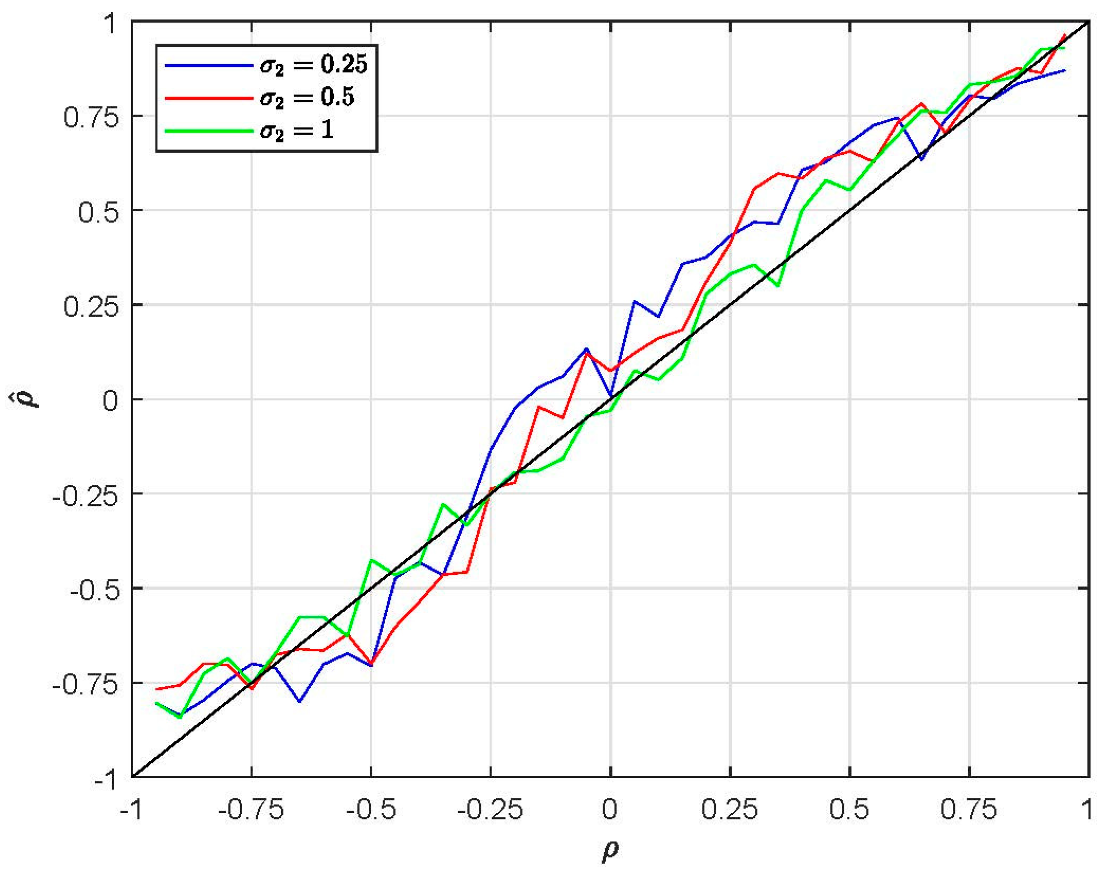
Figure 1 plots the estimated $\widehat{\rho }$ against its true values, which ranges from −0.95 to 0.95 with increments of 0.05, where $\widehat{\rho }$ is calculated as the averages of $\rho$ MSL estimates under M0 specification, obtained based on 100 samples ($R=100$) generated for the same set of true values and estimated with 1000 Halton draws ($H=1000$). The diagonal black line represents the true value of $\rho$. The blue, red and green lines correspond to ${\sigma }_2=0.25$, ${\sigma }_2=0.5$ and ${\sigma }_2=1$, respectively. Figure 1 shows that $\widehat{\rho }$ is mostly biased downward for $H=1000$.

Finally, when the researcher erroneously assumes that the true correlation is zero (M1), there is no substantial worsening in the performance of the MSL estimates. Similarly, when $\rho$ is restricted at the true values (M2), there is no substantial improvement in the estimation of the parameters. A potential explanation for this is that the biases in the MSL estimation of taste patterns are mostly caused by difficulties in estimating the correlation parameter, with the efficiency of the $\rho$ estimates declining for smaller values of ${\sigma }_2$.

4.2. Substitution Patterns: EC2 Simulation Evidence

Table 2. MSL estimates for EC2 (substitution patterns).

		$\mathit{\rho }\mathbf{=}\mathbf{-}\mathbf{0.95}$
		250 Draws			500 Draws			1000 Draws
		${\mathit{\sigma }}_{\mathbf{2}}\mathbf{=}\mathbf{0.25}$	${\mathit{\sigma }}_{\mathbf{2}}\mathbf{=}\mathbf{0.5}$	${\mathit{\sigma }}_{\mathbf{2}}\mathbf{=}\mathbf{1}$	${\mathit{\sigma }}_{\mathbf{2}}\mathbf{=}\mathbf{0.25}$	${\mathit{\sigma }}_{\mathbf{2}}\mathbf{=}\mathbf{0.5}$	${\mathit{\sigma }}_{\mathbf{2}}\mathbf{=}\mathbf{1}$	${\mathit{\sigma }}_{\mathbf{2}}\mathbf{=}\mathbf{0.25}$	${\mathit{\sigma }}_{\mathbf{2}}\mathbf{=}\mathbf{0.5}$	${\mathit{\sigma }}_{\mathbf{2}}\mathbf{=}\mathbf{1}$
M0	${\widehat{\alpha }}_1$	−0.274	−0.271	−0.241	−0.278	−0.246	−0.243	−0.285	−0.266	−0.238
		(0.012)	(0.012)	(0.012)	(0.011)	(0.012)	(0.012)	(0.012)	(0.011)	(0.012)
	${\widehat{\alpha }}_2$	−0.341	−0.299	−0.227	−0.321	−0.289	−0.233	−0.349	−0.301	−0.216
		(0.011)	(0.013)	(0.012)	(0.014)	(0.015)	(0.014)	(0.014)	(0.013)	(0.012)
	$\widehat{\beta }$	1.160	1.127	1.078	1.165	1.126	1.071	1.146	1.127	1.069
		(0.009)	(0.009)	(0.010)	(0.009)	(0.010)	(0.009)	(0.008)	(0.008)	(0.009)
	${\widehat{\sigma }}_2$	0.258	0.469	0.892	0.284	0.484	0.874	0.252	0.442	0.853
		(0.055)	(0.050)	(0.044)	(0.058)	(0.060)	(0.044)	(0.053)	(0.050)	(0.043)
	$\widehat{\rho }$	−0.781	−0.810	−0.799	−0.826	−0.740	−0.819	−0.805	−0.768	−0.803
		(0.040)	(0.034)	(0.036)	(0.037)	(0.039)	(0.033)	(0.034)	(0.035)	(0.036)
M1	${\widehat{\alpha }}_1$	−0.243	−0.200	−0.095	−0.247	−0.188	−0.093	−0.255	−0.199	−0.095
		(0.009)	(0.009)	(0.009)	(0.009)	(0.009)	(0.010)	(0.010)	(0.010)	(0.009)
	${\widehat{\alpha }}_2$	−0.285	−0.241	−0.161	−0.292	−0.244	−0.171	−0.312	−0.247	−0.161
		(0.010)	(0.011)	(0.013)	(0.013)	(0.013)	(0.016)	(0.011)	(0.013)	(0.013)
	$\widehat{\beta }$	1.153	1.111	1.085	1.157	1.117	1.080	1.132	1.113	1.084
		(0.010)	(0.009)	(0.011)	(0.009)	(0.011)	(0.012)	(0.008)	(0.010)	(0.011)
	${\widehat{\sigma }}_2$	0.335	0.534	1.199	0.452	0.660	1.199	0.365	0.558	1.211
		(0.052)	(0.053)	(0.058)	(0.049)	(0.053)	(0.060)	(0.041)	(0.050)	(0.055)
M2	${\widehat{\alpha }}_1$	−0.283	−0.280	−0.278	−0.283	−0.265	−0.281	−0.291	−0.278	−0.278
		(0.012)	(0.012)	(0.013)	(0.012)	(0.013)	(0.010)	(0.013)	(0.011)	(0.013)
	${\widehat{\alpha }}_2$	−0.319	−0.312	−0.308	−0.319	−0.303	−0.319	−0.347	−0.316	−0.308
		(0.013)	(0.015)	(0.016)	(0.016)	(0.017)	(0.019)	(0.015)	(0.016)	(0.016)
	$\widehat{\beta }$	1.160	1.134	1.123	1.160	1.129	1.117	1.144	1.135	1.123
		(0.010)	(0.010)	(0.011)	(0.010)	(0.011)	(0.011)	(0.009)	(0.010)	(0.011)
	${\widehat{\sigma }}_2$	0.235	0.452	1.027	0.223	0.449	1.058	0.222	0.451	1.028
		(0.048)	(0.047)	(0.055)	(0.052)	(0.053)	(0.044)	(0.045)	(0.045)	(0.055)

presents the M0, M1, and M2 results for the EC2 simulations when the true correlation is $\rho =-0.95$. First, notice that increasing the true value of variance ${\sigma }_2$ in M0 reduces the bias in ${\alpha }_1$, ${\alpha }_2,$ and $\beta$. For example, given the estimated ${\alpha }_1$, ${\alpha }_2,$ and $\beta$ as −0.274 (0.012), −0.314 (0.011), and 1.16 (0.009), respectively, we may reject the null hypotheses that $H_o:{\alpha }_2=-0.25$ and $H_o:\beta =1$. However, when we increase ${\sigma }_2$ to one, the estimated ${\alpha }_1$, ${\alpha }_2,$ and $\beta$ are within 3 standard errors of their respective true values. This conclusion is irrespective of the number of Halton draws.

Second, the standard errors for the estimated ${\sigma }_2$ are substantially larger than those for ${\alpha }_1$, ${\alpha }_2,$ and $\beta$. As a result, the estimated ${\sigma }_2$ is within 3 standard errors of its true value across almost all the parameter sets presented in Table 2. Therefore, the null hypothesis that ${\sigma }_2$ is equal to the true value cannot be rejected for almost all the cases. The only exception is the case when ${\sigma }_2=1$ and $H=1000$, and ${\widehat{\sigma }}_2$ is 0.853 (0.043) and it is separated from the true value by 3.4 standard errors. The standard errors decrease slightly when the correlation is restricted in the specifications M1 and M2.

Third, the correlation parameter $\rho$ is estimated with substantial biases in all the M0 specifications. The estimated $\widehat{\rho }$ is separated from the true value by 4 ($H=1000,{\sigma }_2=1$) to 6 standard errors ($H=500,{\sigma }_2=0.25$), and the null hypothesis $H_o:\rho =-0.95$ is rejected in all the cases. The EC2 results for the other 38 correlation values are provided in the Supplementary Materials.

Figure 2 plots the estimated $\widehat{\rho }$ against the true values, once again ranging from −0.95 to 0.95 with increments of 0.05. Although $\widehat{\rho }$ is close to $\rho$ for some values, the estimated correlation parameter mostly displays biases. The biases are smaller for ${\sigma }_2=1$ relative to when ${\sigma }_2=0.25$ or ${\sigma }_2=0.5$. This finding is consistent with that of Jumamyradov and Munkin (2021) for the bivariate normal and bivariate Poisson-lognormal models. They report larger biases for smaller standard deviations. Overall, the M0 results show biases for all five parameters ${\alpha }_1$, ${\alpha }_2$, $\beta$, ${\sigma }_2$, and $\rho$.

It is also interesting to notice that the MSL estimates of ${\alpha }_1$ and ${\alpha }_2$ in M1 have larger biases than in M0 for larger variances, and this is regardless of the number of Halton draws. For example, when $H=250$ and ${\sigma }_2=1$, the estimated ${\alpha }_1$ and ${\alpha }_2$ are −0.095 (0.009) and −0.161 (0.013), and are separated from their true value ${\alpha }_1={\alpha }_2=-0.25$ by 17 and 7 standard errors, respectively. This does not change much for larger numbers of Halton draws. Thus, misspecifying the model setting correlation to $\rho =0$ results in very large biases in ${\alpha }_1$ and ${\alpha }_2$. Moreover, M1 produces larger positive biases for ${\sigma }_2$ compared to M0. For example, when $H=1000$, the estimated ${\sigma }_2$ are 0.365 (0.041), 0.558 (0.050), and 1.211 (0.055), while the true ${\sigma }_2=0.25$, ${\sigma }_2=0.5$ and ${\sigma }_2=1$, respectively. Moreover, the estimates of ${\alpha }_1$, ${\alpha }_2,$ and $\beta$ improve with larger variances in M0; however, we do not observe similar patterns in the M2 estimation, although there is an improvement in the estimation of ${\sigma }_2$.

4.3. Choice Probabilities and Marginal Effects

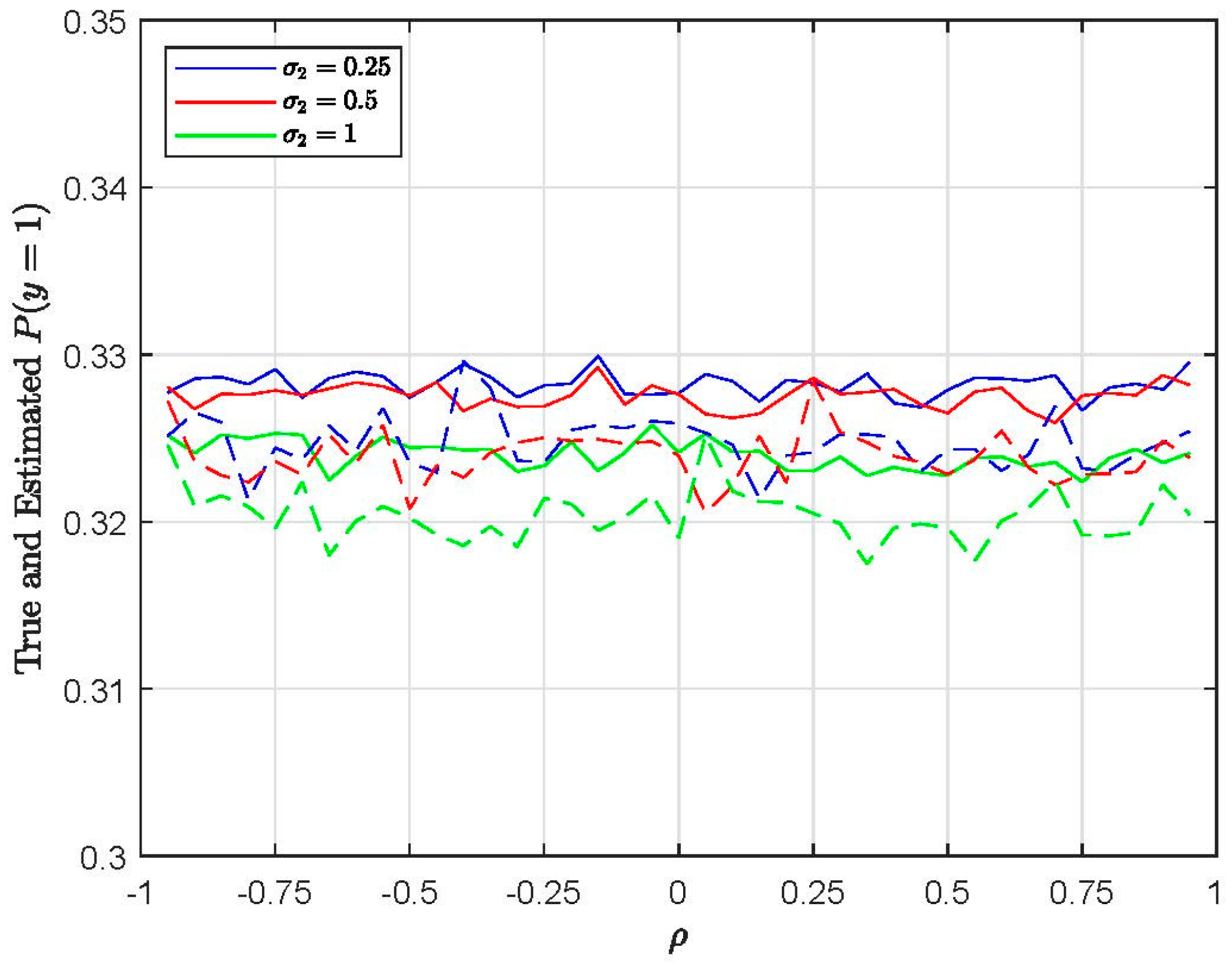
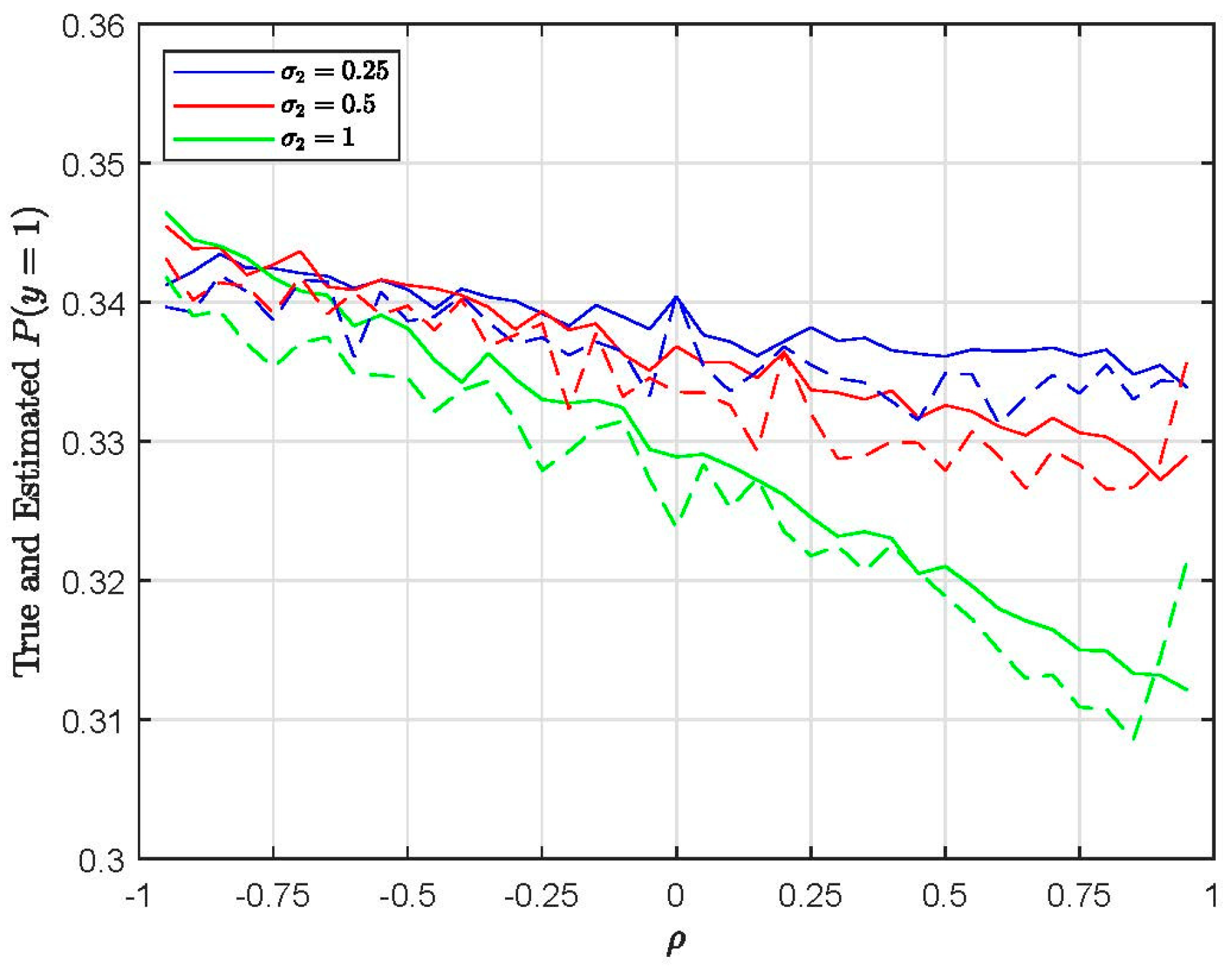
Next, we examine how these reported biases affect the estimated choice probabilities and marginal effects (see Appendix A for the formulas of the marginal effects). Figure 3 plots the true and estimated $P(y=1)$ calculated based on the M0 estimates of the EC1 specification with 500 Halton draws. The true probability means are calculated for the true values of all the parameters. The straight lines represent the true choice probabilities and the dashed lines represent the estimated choice probabilities. Figure 4 plots the true and estimated $P(y=1)$ based on the M0 estimates of the EC2 specification with 500 Halton draws. Even though there are significant biases in the estimated parameters, as expected, the choice probabilities are close to their true values for both the EC1 and EC2 specifications (i.e., taste and substitution patterns).

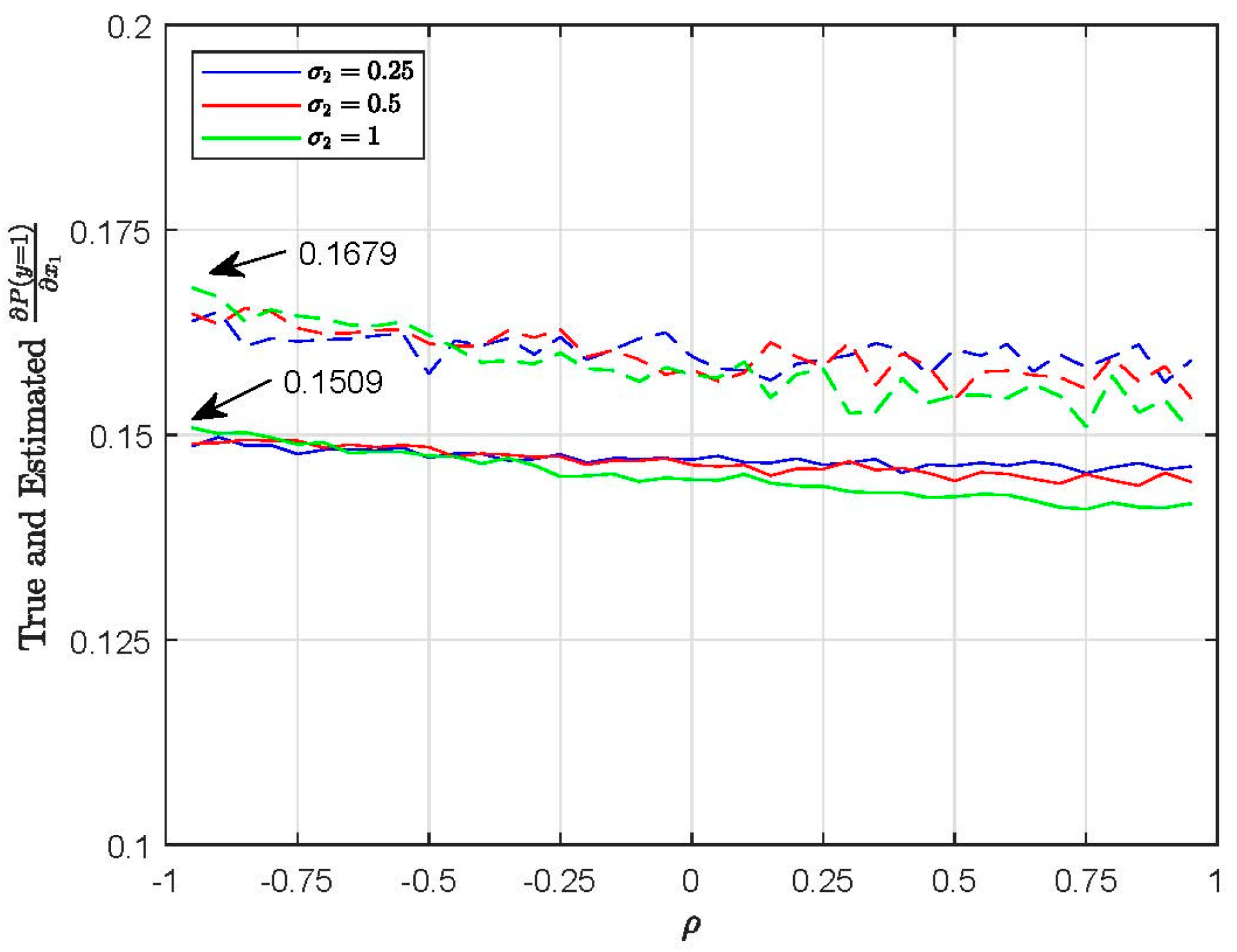
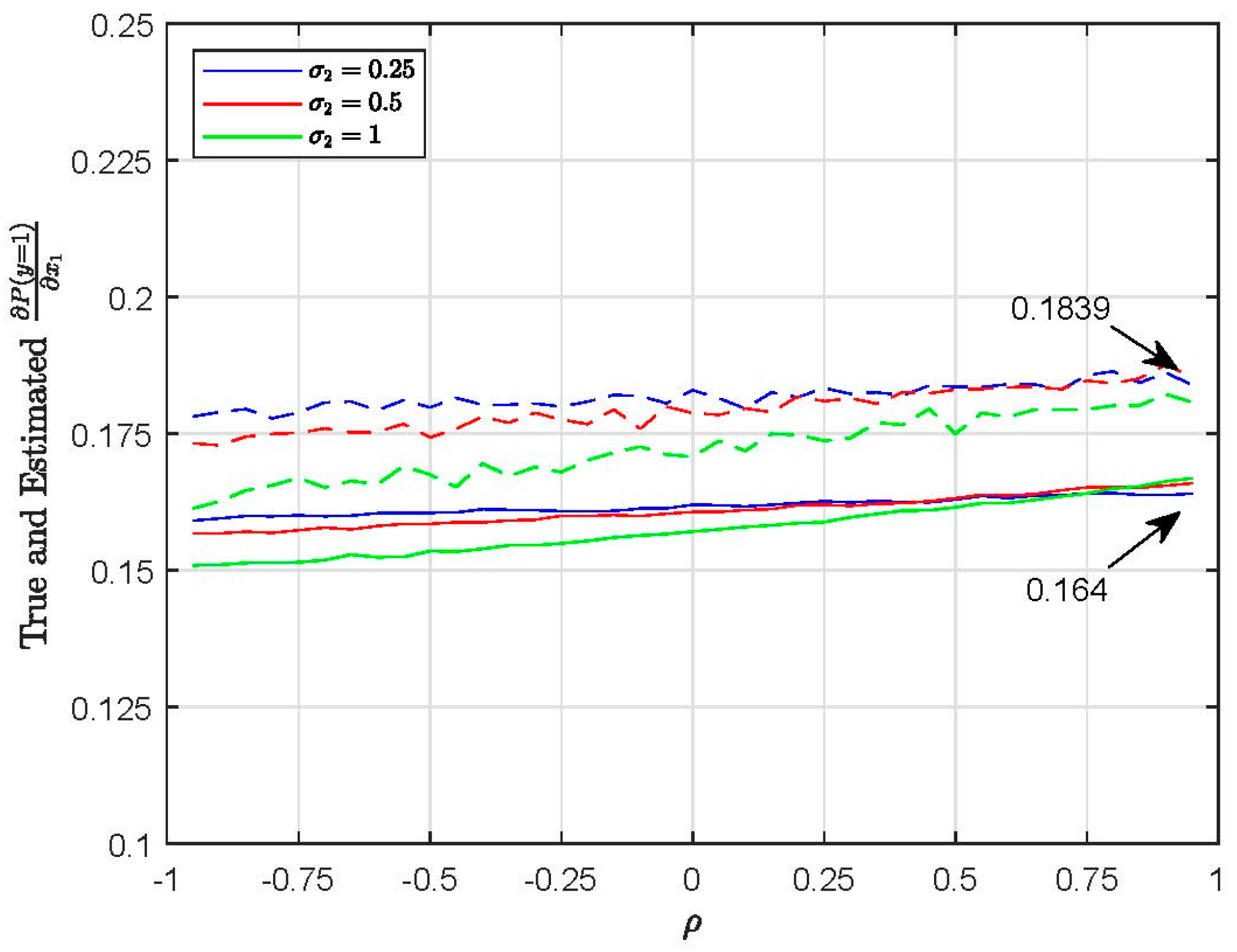
However, when comparing the true and estimated marginal effects, the differences are considerable. Figure 5 plots the true and estimated $\partial P(y=1)/\partial x_1$ for EC1 (M0, 500 Halton draws). For example, when ${\sigma }_2=1$ and $\rho =0.95$, the true $\partial P(y=1)/\partial x_1$ is 0.1509 and the estimated $\partial P(y=1)/\partial x_1$ is 0.1679. Thus, the marginal effect in this case is overestimated by 11%. Figure 6 plots the true and estimated $\partial P(y=1)/\partial x_1$ for EC2 (M0, 500 Halton draws). For example, when ${\sigma }_2=1$ and $\rho =-0.95$, the true $\partial P(y=1)/\partial x_1$ is 0.164 and the estimated $\partial P(y=1)/\partial x_1$ is 0.1839, which is overestimated by 12%.

5. Discussion

In this paper, we examine the properties of the MSL estimator in the context of two MIXL model specifications, EC1 and EC2 (i.e., taste and substitution patterns), where random parameters are generated by a correlated bivariate normal structure. We find that the MSL estimator produces significant biases in the estimated parameters. The problem becomes worse when the true value of the variance parameter is small and the correlation parameter is large in magnitude. Furthermore, we find that the biases in the estimated marginal effects can be as large as 12% of the true values. These biases are largely invariant to increases in the number of Halton draws. Since the existing literature has relied heavily on the MSL estimator in the analysis of the MIXL model, our findings should be an important additional warning to researchers about potential sizable biases in the results.

We also discover that the performance of the MSL depends on other factors, such as the model specification (i.e., EC1 or EC2), distributional assumptions, exogenous variation, as well as the true values of variance and correlation parameters. Therefore, we believe that biases in empirical applications (e.g., discrete choice experiments in health preference research) are likely to be worse due to real-world complexity; however, more research is needed to address such questions. Future simulation studies may examine biases in more complex specifications, such as the generalized MIXL or EC MIXL with more than two random parameters.

References

- Bastin, Fabian, and Cinzia Cirillo. 2010. Reducing simulation bias in mixed logit model estimation. Journal of Choice Modelling 3: 71–88. [Google Scholar] [CrossRef]
- Ben-Akiva, Moshe, Denis Bolduc, and Mark Bradley. 1993. Estimation of travel choice models with randomly distributed values of time. Transportation Research Record 1413: 88–97. [Google Scholar]
- Bhat, Chandra. 1998. Accommodating flexible substitution patterns in multidimensional choice modeling: Formulation and application to travel mode and departure time choice. Transportation Research Part B: Methodological 32: 455–66. [Google Scholar] [CrossRef]
- Bhat, Chandra. 2000. Incorporating observed and unobserved heterogeneity in urban work travel mode choice modeling. Transportation Science 34: 228–38. [Google Scholar] [CrossRef]
- Bhat, Chandra. 2001. Quasi-random maximum simulated likelihood estimation of the mixed multinomial logit model. Transportation Research Part B: Methodological 35: 677–93. [Google Scholar] [CrossRef]
- Boyd, Hayden, and Robert Mellman. 1980. The effect of fuel economy standards on the U.S. automotive market: An hedonic demand analysis. Transportation Research Part A: General 14: 367–78. [Google Scholar] [CrossRef]
- Brownstone, David, and Kenneth Train. 1998. Forecasting new product penetration with flexible substitution patterns. Journal of Econometrics 89: 109–29. [Google Scholar] [CrossRef]
- Cardell, Scott, and Frederick Dunbar. 1980. Measuring the societal impacts of automobile downsizing. Transportation Research Part A: General 14: 423–34. [Google Scholar] [CrossRef]
- Czajkowski, Mikołaj, and Wiktor Budziński. 2019. Simulation error in maximum likelihood estimation of discrete choice models. Journal of Choice Modelling 31: 73–85. [Google Scholar] [CrossRef]
- Debreu, Gerard. 1960. Review of Duncan Luce, Individual Choice Behavior: A theoretical analysis. American Economic Review 50: 186–88. [Google Scholar]
- Elshiewy, Ossama, German Zenetti, and Yasemin Boztug. 2017. Differences between classical and Bayesian estimates for mixed logit models: A replication study. Journal of Applied Econometrics 32: 470–76. [Google Scholar] [CrossRef]
- Fiebig, Denzil, Michael Keane, Jordan Louviere, and Nada Wasi. 2010. The generalized multinomial logit model: Accounting for scale and coefficient heterogeneity. Marketing Science 29: 393–421. [Google Scholar] [CrossRef]
- Gourieroux, Christian, and Alain Monfort. 1990. Simulation based inference in models with heterogeneity. Annales d’Economie et de Statistique 20/21: 69–107. [Google Scholar] [CrossRef]
- Gourieroux, Christian, and Alain Monfort. 1996. Simulation-Based Econometric Methods. New York: Oxford University Press. [Google Scholar]
- Greene, William, and David Hensher. 2010. Does scale heterogeneity across individuals matter? An empirical assessment of alternative logit models. Transportation 37: 413–28. [Google Scholar] [CrossRef]
- Haan, Peter, Daniel Kemptner, and Arne Uhlendorff. 2015. Bayesian procedures as a numerical tool for the estimation of an intertemporal discrete choice model. Empirical Economics 49: 1123–41. [Google Scholar] [CrossRef]
- Hajivassiliou, Vassilis, Daniel McFadden, and Paul Ruud. 1996. Simulation of multivariate normal rectangle probabilities and their derivatives theoretical and computational results. Journal of Econometrics 72: 85–134. [Google Scholar] [CrossRef]
- Hensher, David, and William Greene. 2003. The mixed logit model: The state of practice. Transportation 30: 133–76. [Google Scholar] [CrossRef]
- Hensher, David, John Rose, and William Greene. 2005. Applied Choice Analysis: A Primer. Cambridge: Cambridge University Press. [Google Scholar]
- Hess, Stephane, and John Rose. 2012. Can scale and coefficient heterogeneity be separated in random coefficients models? Transportation 39: 1225–39. [Google Scholar] [CrossRef]
- Hess, Stephane, and Kenneth Train. 2017. Correlation and scale in mixed logit models. Journal of Choice Modelling 23: 1–8. [Google Scholar] [CrossRef]
- Hess, Stephane, Michel Bierlaire, and John Polak. 2005. Estimation of value of travel-time savings using mixed logit models. Transportation Research Part A: Policy and Practice 39: 221–36. [Google Scholar] [CrossRef]
- Huber, Joel, and Kenneth Train. 2001. On the similarity of classical and Bayesian estimates of individual mean partworths. Marketing Letters 12: 259–69. [Google Scholar] [CrossRef]
- Jumamyradov, Maksat, and Murat Munkin. 2021. Biases in maximum simulated likelihood estimation of bivariate models. Journal of Econometric Methods 11: 55–70. [Google Scholar] [CrossRef]
- Keane, Michael, and Nada Wasi. 2013. Comparing alternative models of heterogeneity in consumer choice behavior. Journal of Applied Econometrics 28: 1018–45. [Google Scholar] [CrossRef]
- Lee, Lung-Fei. 1995. Asymptotic bias in simulated maximum likelihood estimation of discrete choice models. Econometric Theory 11: 437–83. [Google Scholar] [CrossRef]
- Lerman, Steven, and Charles Manski. 1980. On the use of simulated frequencies to approximate choice probabilities. In Structural Analysis of Discrete Data with Econometric Applications. Edited by Charles Manski and Daniel McFadden. Cambridge: MIT Press, pp. 305–19. [Google Scholar]
- Louviere, Jordan, Deborah Street, Leonie Burgess, Nada Wasi, Towhidul Islam, and Anthony Marley. 2008. Modeling the choices of individual decision-makers by combining efficient choice experiment designs with extra preference information. Journal of Choice Modelling 1: 128–64. [Google Scholar] [CrossRef]
- Louviere, Jordan, Deborah Street, Richard Carson, Andrew Ainslie, Jay DeShazo, Trudy Cameron, David Hensher, Robert Kohn, and Tony Marley. 2002. Dissecting the random component of utility. Marketing Letters 13: 177–93. [Google Scholar] [CrossRef]
- Louviere, Jordan, Robert Meyer, David Bunch, Richard Carson, Benedict Dellaert, Michael Hanemann, David Hensher, and Julie Irwin. 1999. Combining sources of preference data for modeling complex decision processes. Marketing Letters 10: 205–17. [Google Scholar] [CrossRef]
- McFadden, Daniel. 1974. Conditional logit analysis of qualitative choice behavior. In Frontiers in Econometrics. Edited by Paul Zarambka. New York: Academic Press, pp. 105–42. [Google Scholar]
- McFadden, Daniel. 2001. Economic choices. American Economic Review 91: 351–78. [Google Scholar] [CrossRef]
- McFadden, Daniel, and Kenneth Train. 2000. Mixed mnl models for discrete response. Journal of Applied Econometrics 15: 447–70. [Google Scholar] [CrossRef]
- Palma, Marco, Dmitry Vedenov, and David Bessler. 2020. The order of variables, simulation noise, and accuracy of mixed logit estimates. Empirical Economics 58: 2049–83. [Google Scholar] [CrossRef]
- Quandt, Richard. 1970. The Demand for Travel: Theory and Measurement. Lexington: Heath and Company. [Google Scholar]
- Regier, Dean A., Mandy Ryan, Euan Phimister, and Carlo A. Marra. 2009. Bayesian and classical estimation of mixed logit: An application to genetic testing. Journal of Health Economics 28: 598–610. [Google Scholar] [CrossRef] [PubMed]
- Revelt, David, and Kenneth Train. 1998. Mixed logit with repeated choices: Households’ choices of appliance efficiency level. The Review of Economics and Statistics 80: 647–57. [Google Scholar] [CrossRef]
- Train, Kenneth. 2009. Discrete Choice Methods with Simulation. New York: Cambridge University Press. [Google Scholar]
Figure 1.
Plots of for EC1 (taste patterns) using M0 (H = 1000).
Figure 2.
Plots of for EC2 (substitution patterns) using M0 (H = 1000).
Figure 3.
Plots of true and estimated for EC1 (taste patterns) using M0 (H = 500).
Figure 4.
Plots of true and estimated for EC2 (substitution patterns) using M0 (H = 500).
Figure 5.
Figure 6.