Econometric Fine Art Valuation by Combining Hedonic and Repeat-Sales Information

1
Department of Economics, McGill University, Montreal, QC H3A 2T7, Canada
2
Dépt. de Sciences Économiques, Université du Québec à Montréal, Montréal, QC H2L 2C4, Canada
*
Author to whom correspondence should be addressed.
Econometrics 2018, 6(3), 32; https://0-doi-org.brum.beds.ac.uk/10.3390/econometrics6030032
Submission received: 11 December 2017
/
Revised: 11 April 2018
/
Accepted: 5 June 2018
/
Published: 24 June 2018
(This article belongs to the Special Issue Celebrated Econometricians: Peter Phillips)
Abstract
:Statistical methods are widely used for valuation (prediction of the value at sale or auction) of a unique object such as a work of art. The usual approach is estimation of a hedonic model for objects of a given class, such as paintings from a particular school or period, or in the context of real estate, houses in a neighborhood. Where the object itself has previously sold, an alternative is to base an estimate on the previous sale price. The combination of these approaches has been employed in real estate price index construction (e.g., Jiang et al. 2015); in the present context, we treat the use of these different sources of information as a forecast combination problem. We first optimize the hedonic model, considering the level of aggregation that is appropriate for pooling observations into a sample, and applying model-averaging methods to estimate predictive models at the individual-artist level. Next, we consider an additional stage in which we incorporate repeat-sale information, in a subset of cases for which this information is available. The methods are applied to a data set of auction prices for Canadian paintings. We compare the out-of-sample predictive accuracy of different methods and find that those that allow us to use single-artist samples produce superior results, that data-driven averaging across predictive models tends to produce clear gains, and that, where available, repeat-sale information appears to yield further improvements in predictive accuracy.
JEL Classification:
Z111. Introduction
In the secondary art market, the only way to know with certainty the value placed on an art work at a particular point in time is to see the work be offered for sale and purchased. Nonetheless, there are many art market participants who would like to have an approximate idea of the worth of a work and for whom this datum is unavailable, because the work in question has been sold privately, has not been sold recently, or will not be sold. An owner who is considering offering a work for sale will often want to know what it might fetch before consigning it to an auction house; the valuation of an individual work or indeed an entire collection can be necessary for insurance or taxation.
Although expert appraisers can be consulted, and are employed by auction houses to set the pre-sale estimates reported in auction catalogues, in many cases, expert appraisal may be more costly than necessary given the degree of precision required or the likely value of the work. In such cases, the application of a statistical model that averages over past sale prices of art works that are in some way similar to the one under consideration can provide a quick and relatively inexpensive estimate of the likely sale price. Indeed, there are agencies that provide such estimates on a commercial basis (Artprice.com, Blouin Art Index, and Beautiful Asset Advisors), and statistical models may also be useful in providing a baseline estimate for a professional appraiser.
The usual statistical model of this type is the hedonic regression, in which various observable characteristics of an item are used to estimate its value. Well established in the literature on real estate pricing (see for example Meese and Wallace (1997), and Hodgson et al. (2006)), there is also a body of research that applies hedonic regression to the analysis of the pricing of collectible objects, including art works (see for example Hodgson and Vorkink 2004). In recent real estate literature, hedonic models have also been combined with information from repeat sales of the same property (see in particular Jiang et al. 2015). Hedonic regression is applied when we have a number of observations on sales of objects that, although individually unique, have some degree of commonality, so that the likely value of an item can be inferred from sales of other items. In Hodgson and Vorkink (2004), these objects are paintings created by important (as judged by major art-historical survey books) Canadian painters; Arvin and Scigliano (2004) consider the Canadian Group of Seven painters; Atukeren and Seckin (2009) study Turkish paintings; and Hellmanzik (2009, 2010) studies prominent modern artists. A typical hedonic data set contains sale-specific data such as the price and date of sale (and auction house when the observations come from auction sales), as well as object-specific characteristics such as the size, materials, date of production, and artist and subject matter (in the case of paintings).
Hedonic regressions in the context of a particular art market often group all artists together in one estimation sample, in which most of the hedonic covariates are presumed to have the same proportionate effect on the value of a painting regardless of artist. Differences among artists are captured by individual-artist dummies. Such a specification has clear shortcomings, because the effect on valuation of a given characteristic, for example the age of the artist at the date of execution of the work, may differ across artists; in fact, there is a growing literature that explores the effects of various forms of disaggregation of a large group of artists on the estimated age-valuation profile (e.g., Galenson (2000, 2001), Galenson and Weinberg (2000, 2001), Hellmanzik (2009, 2010), Accominotti (2009), and Hodgson (2011)). The effects of disaggregation by, for example, birth cohort, can be striking. Researchers have generally avoided the estimation of individual-artist level hedonic models, however, because the number of degrees of freedom, although ample in a model where many artists are pooled together, can be prohibitively small at the level of individual artists.
When a work is known to have sold previously, this prior-sale information can also be used to predict the value at the next sale. However, market conditions may have evolved since the previous sale, particularly if it was relatively long ago; combining both types of information may lead to better estimates, as noted earlier with respect to construction of price indices for real estate. Using the hedonic characteristics together with the previous-sale information may be seen as a forecast combination problem.
The present paper investigates the problem of improving upon art valuations from simple hedonic regression methods, using two potential efficiency improvements. First, as in Galbraith and Hodgson (2012), we consider the estimation of hedonic regressions for individual artists with relatively few degrees of freedom by applying model-averaging methods.1 We can then examine whether an artist-specific hedonic model average may be able to deliver hedonic predictions of the sale price of a painting that are superior to those provided by a single model. Second, we suggest methods for incorporating repeat-sale information, where available for a particular work of art, into a hybrid prediction. Both the hedonic model average and hybrid repeat-sale methods are evaluated with respect to predictive performance.
We examine the out-of-sample predictive ability of these methods using auction data for a set of sixty-four prominent Canadian painters over the period 1968–2015. A sequence of rolling estimation samples is used, with all data up to a particular year used to obtain parameter estimates which are then used to predict the prices of all art works for the following year. Data from the years until 2000 are used for initial estimation, and from 2001 to 2015 are used for pseudo-out-of-sample prediction. Measures of prediction loss (such as root mean squared error) are then computed for each method and artist, and comparisons are drawn between the predictive power of alternative methods. Model-average results are compared with simple least-squares regressions, and the usefulness of repeat-sale information is evaluated.
We emphasize that this study makes no claim concerning the relative accuracy of statistical and expert predictions. Instead, our aim is to investigate whether statistical forecasts, based on the limited information sets available to the econometrician, can be made more efficient through econometric methods such as model averaging, and by incorporating repeat sale information where available. The next section of the paper describes the econometric methods, and the data and empirical results are presented in Section 3.
2. Econometric Methods
The econometric valuation of art objects has traditionally relied on hedonic methods, by which the value of an object is assumed to derive from characteristics that are at least in part observable, one of which is the identity of the artist. While these methods have also long been used in real estate valuation, recent literature (particularly with respect to price index construction) has increasingly moved toward estimates based on past sales (the repeat-sales method, RSM), or the combination of hedonic methods with repeat sales.2
There are many similarities between the problems of valuing individual art objects, and real estate. In each case, there is a market for individual items which trade infrequently, and which are individually unique but nonetheless have some degree of commonality with other items. In each case, hedonic models have had some success in capturing characteristics which clearly have important effects on sale prices, but the processes determining the price may differ markedly for different classes of object. In each case, the number of observations which are repeat sales also tends to be a small proportion of a sample of data.
2.1. Hedonic Models
We adopt the notation of Jiang et al. (2015), making only such modifications as are necessary for the problem at hand. Let, therefore, be the logarithm of the price of the ith work of art, sold for the jth time, by artist z. In a large majority of cases, a work is observed to sell only once, and so ; nevertheless, the data set does contain many examples with The date of sale corresponding to this observation is and is observed here only at the level of the year; the last year of the sample is A general hedonic formulation (Jiang et al. 2015, Equation (1)) is:
The are observable characteristics of the work (unchanging with j), which are presumed in a hedonic specification to give utility and therefore affect value. In this specification, there is an artist-specific effect and a work-specific effect as well. This specification is appropriate to a sample that pools the works of all artists; a corresponding specification for an individual artist is
where we now suppress the subscript z since it is a constant within each artist-specific sample. Unless parameters are identical for each in which case the specification in (1) is unambiguously more efficient, there is a bias–variance trade-off between (1) and (2). The small number of repeat sales () in our sample means that we have little information with which to estimate separately from the constant; it is therefore suppressed in our empirical specifications.
Estimation by least squares (LS) is generally straightforward: endogeneity of regressors is not normally a problem in modeling secondary market prices at auctions which take place many years after the determination of characteristics of the artwork (a possible exception to this rule lies in auction house dummy variables, if these are used as characteristics of the work).
The literature on the estimation of art valuation models by hedonic methods, using data from auction sales, is now quite substantial. In general, the logarithm of the sale price of a specific object is regressed on a number of characteristics specific to that sale, such as the date, auction house, artist, medium, support, subject matter, size, etc. Most of the variables are categorical, and so are included as dummy variables, with the number of dummies for each characteristic corresponding with the number of categories associated with the characteristic. For example, in the original data set of Hodgson and Vorkink (2004), comprising part of the data used in the present study, there were over forty auction houses, nine genre categories, over twenty medium/support combinations, and about forty-five annual time-of-sale indicators. In many such studies, the effects on the price associated with these variables are of central substantive interest. Hodgson (2011) is an example which focuses on pooled age-valuation profiles. Of course, the effects of hedonic characteristics at an individual-artist level could well be different for each artist, and better models may result from using separate models for each. Nonetheless, individual-artist level sample sizes may be too small for reliable estimation by OLS where a relatively large number of hedonic covariates may be present; methods such as those described in the next subsection can alleviate this problem.
2.2. Model Averaging
The common problem of uncertainty concerning model specification particularly afflicts hedonic models of art sales where, as here, we have a large set of potential explanatory variables. In the pooled sample of nearly 10,000 observations, there are sufficient degrees of freedom to include all regressors; by contrast, if we wish to allow all parameters to differ by artist, the number of degrees of freedom for each individual is too small to allow inclusion of all observable indicators. In this case, we need to consider subsets of the possible regressors, but with many available indicators it may be unclear which to include for optimal prediction.
One approach to conserving degrees of freedom that has been successful in a number of forecasting contexts is model averaging, where results from models with different sets of included regressors are averaged, as opposed to choosing only one of the models; model averaging allows us to use information from a large number of potential explanatory effects even where sample sizes preclude including each one in a single regression.3
Model averaging is usually accomplished using sample-based criteria, such as information criteria, to select weights. Hansen (2007) proposed an alternative weighting based on the Mallows (1973) criterion. Within a class of discrete averaging estimators, Hansen showed that this criterion has a minimum mean squared error property, and we adopt this criterion here. For use as a forecasting procedure, we retain the parameter estimates from each of the estimated models with its corresponding weight, produce forecasts from each of the sets of parameters, and produce an overall forecast by weighting these forecasts by the set of model weights.
Galbraith and Hodgson (2012) use the model-average method in the context of artists’ age–valuation profiles, and summarize the steps as follows, but see Hansen (2007) for a detailed exposition. Consider, in the notation of Hansen, the model
where W represents a dimensional set of potential explanatory variables; the columns of W are ordered in accordance with an a priori view of their importance. Select a maximum number M of regressors to include, such that where N is the sample size, and estimate all models with constant and m regressors, The model average estimator of is where is the weight given to model and is the parameter vector estimated using a model with m regressors, padded with zeroes for excluded variables in the cases for which The weights are chosen to minimize the Mallows criterion where is replaced with an estimate and where is the effective number of parameters, being the number of parameters estimated in model
Let the vector of forecasts from model m be Then, the model-average forecast is
again with
2.3. Combining Hedonic and Repeat-Sale Information
For most works in our sample, the base hedonic model, or averages over different hedonic models, will constitute the full set of alternatives that we have sufficient information to consider. In a subset of cases, however, we will have additional information arising from a previous sale of a work. In that case, the question arises as to how, if at all, this additional information should be used. Our approach will be to use forecast combination methods.
A traditional statistical principle states that, when one has information from multiple different sources, it is in general optimal to combine information from the different sources rather than to use one of them alone. In the special case where independent unbiased sources have known finite variances, and one is interested in minimizing the overall variance of a prediction, it is optimal to combine the sources in inverse proportion to their variances (Bates and Granger 1969).
Here, albeit in a relatively small subset of the cases in our data set, we identify a previous sale of a given artwork earlier in the data set which can serve as the basis of an alternative forecast. We make this identification by searching for a previously-sold work by a given artist that has identical measured characteristics. This means that we could in principle incorrectly identify as a match two different works with identical dimensions, year of production, medium, genre and so on; the converse error, failing to identify a genuine repeat sale, should never arise unless there are undiscovered coding errors in the characteristics.
The previous sale price, updated with any information we have concerning changes in average prices over the relevant time period, provides an alternative forecast of the current value at auction. We treat the incorporation of this information, where available, in the classical forecast combination framework.
For sales of art works for which a previous sale can be identified in the data set, let be the hedonic regression forecast of the log price, and be the repeat-sale forecast which, allowing for the different time period effect, is
A combined forecast is then
An optimal weight may be estimated by training based on cases observed at times preceding However, it has often been observed in the literature on forecast combination (see for example Clemen 1989 for a review) that it is difficult to improve upon equal weighting () for two forecasts that are close to being of equal variance. The small individual-artist sample sizes here constrain us to use this equal weighting in this problem, although in large data sets we would expect further efficiency gains from optimization over
Note that the hedonic forecast may be derived from any of the forms of regression model used here: an OLS regression on core variables only, a broader regression involving as many covariates as possible, or a model average over a number of such regressions. We report results below in which repeat-sales forecasts are combined with those derived from both single-regression and model-average methods.
3. Empirical Predictions of Value at Auction
The data set that we use for empirical comparison of methods is an extended version of that used by Hodgson (2011) in a study of age-valuation profiles for Canadian painters. In the pooled model, all of the artists included in the sample are grouped together, whereas, in the individual-artist models, a separate regression is estimated for each artist. The artists included, along with numbers of observations, are listed in Appendix A. For each of the sixty-four painters analyzed, we record every sale of an oil or acrylic work sold at auction during the years 1968–2015 for which date of execution was provided in the auction record, with data also collected on the variables mentioned below. The sources for the data are summaries of sales of Canadian paintings at auction, as reported in Campbell (1970–1975, 1980), Sotheby’s (1975, 1980), and Westbridge (1981–2015). Painters from various periods of Canadian art history are considered, with artists of different gender and working in a variety of styles, and of different geographical and linguistic backgrounds.
The full pooled sample size comprises 9891 works, individual sample sizes range from 50 to 997 with a median of 107, and we have as many as 80 regressors, many of which are indicators for qualitative features of the work of art.
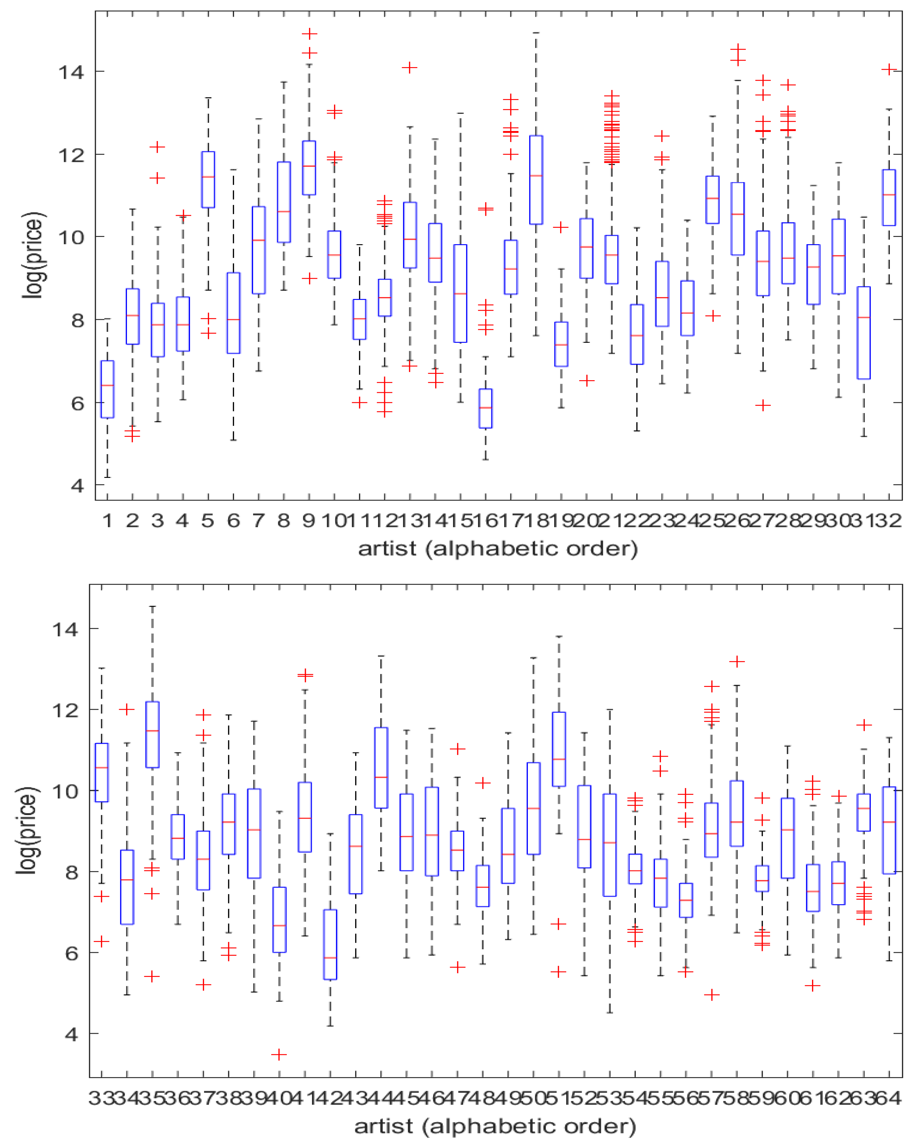
Densities of values of paintings are generally heavily right-skewed; correspondingly, models are usually defined on the logarithms of prices. Figure 1 shows boxplots of the log prices. We see that, as is typical in data on sale prices of works of art, there is wide variation in the locations and dispersions of the 64 distributions, and that there is relatively modest evidence of remaining asymmetry in the logarithmically transformed prices.
3.1. Model Elements
Hedonic models for the prices of art works are usually estimated with the dependent variable as log-price of the sale of a painting at auction, and a (possibly large) set of independent variables that includes the artist’s age at the time of execution of the painting (in polynomial form); the height, width, and surface area of the painting; and dummy variables for the date of the sale, the medium/support combination, the genre of the painting’s subject matter, and, in specifications where different artists are pooled together, for artist identity.
In the literature on the age-valuation relationship, age generally enters as a polynomial function with two to four terms, reflecting the modeling of age–wage or experience–wage profiles in the labour economics literature (e.g., Mincer 1974). Hodgson (2011) estimates a fourth-order polynomial for the overall and cohort regressions, as well as for the specification with continuously shifting profile. Galenson (2000) allows for up to three polynomial terms in each individual-artist regression, selecting order by Here, we include a quadratic specification for each artist.
Table 1 records features of the in-sample fit for the pooled model to give some indication of the relative importance of effects. Table 1a gives parameter estimates for the core variables height, width and area of the work of art, and age, age squared of the artist at the time of execution. Table 1b gives the overall and the degree to which declines with the elimination of different groups of explanatory variables.
Apart from individual-artist dummies, crucial in pooled models, we see that the dimensions of the work (primarily height and width, although the shape information implied in the area measure has a discernible effect) are dominant effects, the elimination of which from the model produces much larger reduction in than all medium and genre indicators, for example. The artist’s age, reflecting career stage, is less clearly important in the pooled sample, but in individual-artist regressions there are cases where this effect is of substantial importance.
3.2. Forecast Evaluation
We have data on auctions that take place over T periods of time (years): we choose a break point, and initially estimate the model for all data observed for . The resulting vector of parameter estimates is then used to calculate an out-of-sample price prediction for each painting i sold in the period , using the fitted values from each forecasting model F1-F6 given in the next sub-section; in the cases of methods F5 and F6, a further step is made in which repeat-sale information is used. The quality of each prediction will be judged by a comparison of the model’s fitted value with the realized auction price for the painting. The only unusual aspect arising here is that, for any painting observed in period , we do not have a parameter estimate for the appropriate time dummy (in the pooled models in which these are used), as of course this dummy did not appear as a regressor in the estimation sample that extended only to period There are various ways to deal with this problem where time dummies are used; in principle, a forecasting model could be applied to use the time dummies for periods to compute a time series forecast of the dummy. We will suppose however that market values can be approximated by a simple random-walk process and use the estimated time dummy for as our forecast of that for 6
The above procedure is then repeated with the estimation sample extended to and predictions of sale prices in period and so on. The data set does not contain information on the month or date of sale, so no timing distinction is made among sales taking place in a given year. Our initial estimation sample comprises data up to and including the year 2000 , and predicted values are computed recursively for the years 2001 through 2015. This method is first applied to the data for all artists pooled together, where at each stage the model is estimated by OLS. We then estimate the regressions at the individual-artist and pooled levels, as described in detail in the next sub-section.
After computing forecasts for each observation in the successive out-of-sample periods 2001–2015, we compute overall measures of forecast loss. In particular, we report the root mean squared error (RMSE), where there are forecasts to evaluate. Because the loss associated with an inaccurate forecast may be asymmetrical—in the case where a forecast is made for a potential seller, for example, it may be more costly to underestimate the potential sale price at auction than to overestimate it—we also report a widely used asymmetric loss function, the linex (linear-exponential) loss, in the form where a is a shape parameter which we set to −0.5.
In principle, the measure used to compare predictive accuracy of different methods could use a loss function motivated by the specific economic use to which the predictions, or appraisals, are being put. In the introduction we gave the three examples of an owner who needs an estimate or appraisal in order to set a sale price (or to decide whether to sell), to insure the object, or to assess it for tax purposes. In all three cases, if we suppose a risk-averse agent, then the ex ante risk exposure of the agent is more or less directly related to the variance of the appraisal error. In the case of the second and third motivations, if we suppose the amount for which the work is to be insured, or the amount of tax that will be paid, is linearly dependent on the appraisal, then the variance of the agent’s financial exposure is directly related to the variance of the appraisal error, so that the use of a MSE loss function may be viewed as a reasonable proxy for an economic measure of loss. In the case of pre-sale appraisal, large over- and under-estimates are both costly to the potential seller, for different reasons, and so even here the MSE seems to be a reasonable proxy for the agent’s loss function, the exact form of which might be complicated and dependent on several case-specific factors. The supplementary linex results help to address cases where asymmetry may be more important; our use of a negative value for the parameter a in this loss function implies greater (exponential) weight on cases where there is underestimation of value, i.e.,
3.3. Predictive Results
We now consider whether refinements of the standard hedonic technique allow us to improve forecasts, on the sub-sample of 5157 observations in the period 2001–2015 used for pseudo-out-of-sample evaluation, as described above. We compare the standard pooled OLS regression on all available regressors (“OLS-pooled, broad”) and individual-artist regressions using one of five specifications: the largest set of regressors which can be included (“OLS-broad”), a minimal OLS model involving only the core characteristics of painting height, width and area, a quadratic polynomial in artist’s age at completion of the painting and a linear time trend (“OLS-core”), the Hansen–Mallows model average (“model average”), and finally the equally weighted combination of repeat-sales information with each of the two previous methods. Using the notation for the core set of six explanatory regressors (year of sale, height, width and surface area of the work, artist’s age and age squared at the time of execution) and for the remaining “non-core” regressors (largely indicators for genre, medium, support, and related characteristics), the different forecasts are computed as follows:
- F1. OLS pooled, broad:
- F2. OLS individual artist, broad:
- F3. OLS individual artist, core:
- F4. Model average: where W contains various combinations of the variables contained in and , with data-based weights as described in Section 2.2.
- F5. OLS core (F3) + RSM: where is the forecast from F3 and is the repeat-sale estimate as given in Equation (5).
- F6. Model average (F4) + RSM: where is the forecast from F4 and is the repeat-sale estimate as given in Equation (5).
In the latter two of these cases, we again report in Table 2 the global results on the set of 5157 test cases, although repeat-sale information is available only in about one-fifth of these cases. Results specific to the cases where repeat sales are identified are reported in Table 3.
The empirical results address several questions:
- Do pooled or individual-artist regressions produce the lower forecast loss? Table 2 summarizes this information.
- Does incorporation of repeat-sale information offer potential further improvement? Table 3 treats the subset of cases in which repeat-sale information is available, compares estimated forecast losses, and gives tests of the null of equal forecast variance with and without repeat-sale information. Figure 2 displays, for each artist, performance of the hybrid model relative to two forms of hedonic model.
- What are the key observable factors that predict sale prices at auction?
Table 2 reports bias and RMSE for the estimators. There are at least a couple of noteworthy points. First, the individual-level regressions show similar negative biases; these may be attributable in large part to the rudimentary treatment of time effects in the individual-artist regressions: the small sample sizes require use of a simple linear trend, rather than individual-year time dummies. In addition, our data set contains only the year of sale (rather than a precise date). In real-time valuation exercises, or in a data set that contained precise daily or monthly dates of sale and sufficient observations to estimate current-date price levels, it should be possible to make such biases smaller. Second, we note the bias-variance trade-off in using the model average estimators. By averaging over some models which are poorer approximations, bias is increased; however, variance is reduced by the usual effect of averaging. We see this in both the pure model average results and in those combining model averaging with repeat-sales information. The net effect on RMSE is negative (i.e., an improvement).
Table 2b clearly suggests that, for symmetric loss cases, results at the individual-artist level tend to be superior to pooled results. Of course, this is a function of sample size; in much smaller sample sizes, pooled models would presumably dominate, while individual models would be more clearly superior in much larger samples. The preferred model is an individual-level model-average forecast that incorporates repeat-sale information where available, whichever of the loss functions one uses. Statistical inference on these differences is provided in Table 3.
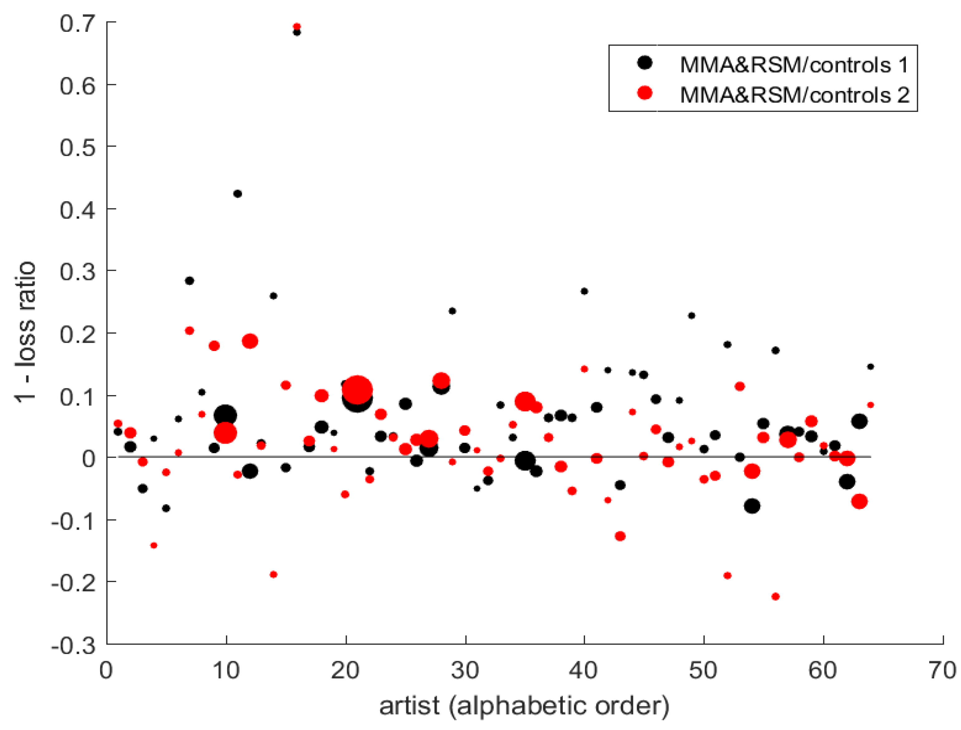
Figure 2 shows a sequence of forecast RMSE loss reductions, [1-loss(model average+repeat sales)/loss(single hedonic model)], across the sample of sixty-four artists (i.e., positive values indicate an improvement in forecast performance measured by RMSE). Linex results are qualitatively similar and are not depicted. Model averaging plus repeat-sales information (“MMA+RSM”) is compared with two alternative hedonic regression models with explanatory variables chosen a priori; the first includes as broad a set of indicator variables as is feasible on the limited sample for the particular artist, and the second is OLS-core.8
Although it is clear from the overall results (Table 2) that the refinements (model averaging, repeat sales) tend to produce some gains, there is considerable variation in results across individual artists visible in the figure, and numerous artists for whom simple hedonic models provided slightly better results in this sample.
Table 4 provides Diebold and Mariano (1995) test results. These test statistics do not account for parameter uncertainty, and so can be expected to be liberal, but are nonetheless indicative of differences.
The superior results produced by model averaging, alone and in combination with repeat-sale information, show strong statistical significance. The difference between model averaging without RSM, and OLS-core using RSM but not model averaging, is insignificant, reflecting the small difference between the forecast loss measures in Table 2; recall however that RSM can only be employed on approximately one-fifth of the cases, limiting the power of the test. Nonetheless, OLS-core + RSM is significantly superior to all methods without RSM, and model averaging + RSM is significantly superior to all other methods.
The impact of incorporation of repeat-sale information may be obscured by the fact that only in a minority of cases can a previous sale can be identified. Table 3 focuses on the subset of 1043 cases for which a repeat sale was identified, to judge the “undiluted” impact of incorporation of this information.
Table 3 reinforces the earlier results. Hedonic model averaging combined with repeat sale information produces the lowest forecast loss, although the difference relative to the core OLS model, also with repeat-sales information, is not significant at conventional levels. The use of repeat-sales information alone, or a hedonic model alone, produces results which are clearly dominated by the combined forecasts.
Globally, there is clear evidence in these data of moderate but statistically genuine improvements in predictive efficiency resulting from the refinement of the hedonic method through model averaging, and the combination with repeat-sale information, where available.
Finally, we draw attention to the simplest of the hedonic regressions, the core model containing painting dimensions, time, and a polynomial in the age of the artist at time of execution of the painting; the age variables capture the period in an artist’s career at which the work was executed, commonly an important factor in the price of the work. Returning to the loss measures of Table 2, we see that simple hedonic models describing the physical dimensions of the painting, time of sale and period in the artist’s career are not far from the best-performing valuation methods that we can identify; that is, these factors evidently capture a large proportion of the explanatory power of the hedonic models.
4. Concluding Remarks
Simple least-squares hedonic regressions are commonly used for quick statistical estimates of the value of a unique object such as a work of art. However, refinements of the simple method, some of which have been employed in the literature on real estate price index construction, are feasible and appear to be potentially valuable.
The main refinements suggested here—weighted model averaging (especially to allow estimates at lower levels of aggregation) and incorporation of repeat-sale information in some form along with hedonic information—are straightforward to implement as well. We find that, with the aid of model-averaging methods, we are able to obtain useful estimates and predictions at a higher level of disaggregation than would otherwise be possible. The application of this approach may well be valuable in other areas where pooled hedonic models are used for appraisal and predictive purposes, for example real estate, where disaggregation at very specific geographical levels, such as postal codes, may be possible and interesting.
While it remains to be seen whether the efficiency gains that we observe here will also be observed in other data sets, the fact that these methods allow the incorporation of additional information suggests that we should expect such efficiency improvements to be a general phenomenon. We have noted also that the incorporation of repeat-sale information here is subject to a number of constraints in the data, and that further reductions in forecast loss are likely to be available. In particular, larger sample sizes would permit optimization over the weights on hedonic models and prior-sale forecasts.
It is noteworthy that hedonic regressions using physical dimensions of the painting, time of sale and period of an artist’s career appear to capture a very large proportion of available predictive power, so that simple hedonic models may perform reasonably well. Nonetheless, both in the hedonic regressions and in combination with repeat-sales information, data-driven averaging across a number of predictive models produces significantly better results than does the use of any single model or predictor.
Author Contributions
Both authors contributed equally to the paper.
Acknowledgments
We thank the Editors and two referees for valuable comments and suggestions. For their comments on early versions of this paper, we thank Vincent Boucher, Bronwyn Coate, Douglas Noonan, and seminar participants at the 2012 Canadian Economics Association Annual Congress, 2012 International Conference for Cultural Economics, 2013 Computational and Financial Econometrics Conference, 2013 North American Cultural Economics Workshop, and 2015 Bilbao Cultural Economics Conference. We also thank the Fonds québécois de la recherche sur la société et la culture (FQRSC) and the Social Sciences and Humanities Research Council of Canada (SSHRC) for financial support of this research, and the Centre Interuniversitaire de recherche en analyse des organisations (CIRANO) for research facilities.
Conflicts of Interest
The authors declare no conflict of interest.
Appendix A
The following are the 64 artists included in our sample, together with the number of sample points (works sold at auction) for each artist.
William Atkinson 83; Maxwell Bates 163; William Beatty 107; Leon Bellefleur 152; Frederic Martlett Bell-Smith 53; André Bieler 61; Paul-Emile Borduas 75; Franklin Brownell 61; Jack Bush 94; Frank Carmichael 61; Emily Carr 135; A.J. Casson 573; F.S. Coburn 293; Charles Comfort 83; Stanley Cosgrove 282; Maurice Galbraith Cullen 92; Jean Dallaire 63; Jacques de Tonnancour 58; Marcelle Ferron 109; Marc-Aurèle Fortin 97; Louise Gadbois 65; Clarence Gagnon 145; John Hammond 146; Lawren Harris 216; Robert Harris 52; Edwin Holgate 80; Yvonne McKague Housser 50; E.J. Hughes 126; A.Y. Jackson 997; Otto Jacobi 88; Frank Johnston 160; Illingworth Kerr 294; Dorothy Knowles 90; Cornelius Krieghoff 185; William Kurelek 68; Jean-Paul Lemieux 184; Rita Letendre 111; Arthur Lismer 382; J.E.H. MacDonald 333; J.W.G. MacDonald 62; Henri Masson 289; Jean McEwen 140; David Milne 112; Norval Morriseau 163; Kazuo Nakamura 51; Toni Onley 74; Paul Peel 73; Robert Pilot 330; George Reid 77; Jean-Paul Riopelle 468; Goodridge Roberts 177; Albert Robinson 122; William Ronald 105; Allen Sapp 176; Jack Shadbolt 172; Gordon Smith 98; Jori Smith 62; Marc-Aurèle Suzor-Coté 148; Takao Tanabe 70; Fernand Toupin 55; Harold Town 125; Fred Varley 59; Frederick Verner 96; W.P. Weston 120.
References
- Accominotti, Fabien. 2009. Creativity from interaction: Artistic movements and the creativity careers of modern painters. Poetics 37: 267–94. [Google Scholar] [CrossRef]
- Arvin, B. Mak, and Marisa Scigliano. 2004. Hedonic prices in art and returns to art investment: Evidence from the Group of Seven at auction. Économie Appliquée 57: 137–62. [Google Scholar]
- Atukeren, Erdal, and Aylin Seckin. 2009. An analysis of the price dynamics between the Turkish and the international paintings markets. Applied Financial Economics 19: 1705–14. [Google Scholar] [CrossRef]
- Bates, J. M., and C. W. J. Granger. 1969. The combination of forecasts. Operational Research Quarterly 20: 451–68. [Google Scholar] [CrossRef]
- Campbell, H. 1970–1975. Canadian Art Auction Record 1969–1974. Toronto: Canadian Antiques and Fine Arts, Montreal: Bernard Amtmann, vols. 1–6. [Google Scholar]
- Campbell, H. 1980. Canadian Art Auctions, Sales, and Prices, 1976–1978. Don Mills: General. [Google Scholar]
- Clapp, John M., and Carmelo Giaccotto. 2002. Evaluating house price forecasts. Journal of Real Estate Research 24: 1–26. [Google Scholar]
- Clemen, Robert T. 1989. Combining forecasts: A review and annotated bibliography. International Journal of Forecasting 5: 559–83. [Google Scholar] [CrossRef]
- Diebold, Francis X., and Roberto Mariano. 1995. Comparing predictive accuracy. Journal of Business and Economic Statistics 13: 253–65. [Google Scholar]
- Galbraith, John W., and Douglas J. Hodgson. 2012. Dimension reduction and model averaging for estimation of artists’ age-valuation profiles. European Economic Review 56: 422–35. [Google Scholar] [CrossRef]
- Galenson, David W. 2000. The careers of modern artists. Journal of Cultural Economics 24: 87–112. [Google Scholar] [CrossRef]
- Galenson, David W. 2001. Painting Outside the Lines. Cambridge: Harvard University Press. [Google Scholar]
- Galenson, David W., and Bruce A. Weinberg. 2000. Age and quality of work: The case of modern American painters. Journal of Political Economy 108: 761–77. [Google Scholar] [CrossRef]
- Galenson, David W., and Bruce A. Weinberg. 2001. Creating modern art: The changing careers of painters in France from impressionism to cubism. American Economic Review 91: 1063–71. [Google Scholar] [CrossRef]
- Hansen, Bruce. 2007. Least squares model averaging. Econometrica 75: 1175–89. [Google Scholar] [CrossRef]
- Hellmanzik, Christiane. 2009. Artistic styles: Revisiting the analysis of modern artists’ careers. Journal of Cultural Economics 33: 201–32. [Google Scholar] [CrossRef]
- Hellmanzik, Christiane. 2010. Location matters: Estimating cluster premiums for prominent modern artists. European Economic Review 54: 199–218. [Google Scholar] [CrossRef]
- Hodgson, Douglas J. 2011. Age-price profiles for Canadian painters at auction. Journal of Cultural Economics 35: 287–308. [Google Scholar] [CrossRef]
- Hodgson, Douglas J., Barrett A. Slade, and Keith P. Vorkink. 2006. Constructing Commercial Indices: A semiparametric adaptive estimator approach. Journal of Real Estate Finance and Economics 32: 151–68. [Google Scholar] [CrossRef]
- Hodgson, Douglas J., and Keith Vorkink. 2004. Asset pricing theory and the valuation of Canadian paintings. Canadian Journal of Economics 37: 629–55. [Google Scholar] [CrossRef]
- Jiang, Liang, Peter C. B. Phillips, and Jun Yu. 2015. New methodology for constructing real estate prices applied to the Singapore residential market. Journal of Banking and Finance 61: S121–31. [Google Scholar] [CrossRef]
- Mallows, C. L. 1973. Some comments on Cp. Technometrics 15: 661–75. [Google Scholar]
- Meese, Richard A., and Nanacy E. Wallace. 1997. The construction of residential housing price indices: A comparison of repeat-sales, hedonic-regression, and hybrid approaches. Journal of Real Estate Finance and Economics 14: 51–73. [Google Scholar]
- Mincer, Jacob A. 1974. Schooling, Experience, and Earnings. New York: Columbia University Press. [Google Scholar]
- Shiller, Robert J. 2008. Derivatives Markets for Home Prices. NBER Working Paper w13962, National Bureau of Economic Research, Cambridge, MA, USA. [Google Scholar] [Green Version]
- Sotheby’s. 1975. Canadian Art at Auction, 1968–1975. Toronto: Sotheby’s. [Google Scholar]
- Sotheby’s. 1980. Canadian Art at Auction, 1975–1980. Toronto: Sotheby’s. [Google Scholar]
- Westbridge, A. R. 1981–2015. Canadian Art Sales Index, 1977–2014. Vancouver: Westbridge Publications Ltd. [Google Scholar]
| 1. | Galbraith and Hodgson (2012) also use model-average methods, as well as principal components, for the problem of estimating individual-artist age-valuation profiles; the quantities of interest are the parameters of a polynomial in the artist’s age. That paper does not consider the sale-price prediction problem. |
| 2. | Repeat sales occur when the same item is sold at least twice in the given sample data, so that an earlier sale may be used to predict the price of a later one. |
| 3. | Jiang et al. (2015) quote Shiller (2008) as follows: “there are too many possible hedonic variables that might be included, and if there are n possible hedonic variables, then there are possible sets of independent variables in a hedonic regression, often a very large number. One could strategically vary the list of included variables until one found the results one wanted.” Model averaging mitigates this problem, providing results based on objective criteria rather than the investigator’s selections. |
| 4. | The notation “e-x”, (e.g., e-05) means . |
| 5. | The notation “——–” indicates the full model with no excluded variables. “All core” means excluding height, width, area, age and age squared; “all medium, genre” means excluding all indicators for the materials with which the work was executed and all indicators for the genre. indicates the decline in when the particular group of variables is omitted from the model. |
| 6. | In the context of housing markets, forecasting models of the time dimension have been considered by, for example, Clapp and Giaccotto (2002). In many cases of both art and real estate, however, a valuation is made conditional on sales already observed in the current year, so that the time lag between price index update and sale is very small, and any deviation of the price process from a random walk should have correspondingly small effect. |
| 7. | Table 2 records bias, variance and loss function measures by method; in the second part of the table, the best (lowest) forecast loss is in bold for each measure. One large extreme outlier is removed for the individual broad OLS regression and equally-weighted model average, in Table 2 and Table 4 results involving either of these two methods; these methods are not competitive and so rankings are not affected, but removal of the outlier gives a more accurate impression of their typical performance. |
| 8. | The size of dot for each artist is proportional to individual sample size. Results from equally weighted model averages are relatively erratic and so are not depicted. |
| 9. | Table 4 gives Diebold–Mariano statistics for the null of no difference in forecast loss between various pairs of methods; the statistic as used here is the difference in the MSE’s of two forecasts divided by an estimate of the standard error of this difference and is asymptotically Because sales are not ordered within a year, we do not apply any correction for autocorrelation in the denominator. A positive value corresponds with lower mean-square forecast loss for the higher-numbered method. |
Figure 1.
Logarithms of sale prices at auction: 9891 paintings, 64 artists. Each of the individual plots corresponds to one of the 64 artists named in Appendix A, in the order given there.
Figure 1.
Logarithms of sale prices at auction: 9891 paintings, 64 artists. Each of the individual plots corresponds to one of the 64 artists named in Appendix A, in the order given there.

Figure 2.
Reduction in RMSE from model-average+ RSM relative to simple hedonic model. (The figure displays [1 - RMSE(combined model average + RSM)/RMSE(hedonic model)] for the 64 artists named in Appendix A. Positive values therefore indicate reduced loss (superior performance) of the model average, with repeat sales where available, relative to the single OLS hedonic model for a particular artist. Model 1 is the hedonic regression with selected dummies + painting dimensions, surface area, age of artist at time of execution, and age squared. Model 2 is the same without dummies. The sizes of dots are proportional to total sample sizes for the artist.)


Table 1.
(a) Estimated coefficients on core variables, in-sample: full sample of 9891 sales, pooled model4; and (b) and from full model and models with excluded variables: full sample of 9891 sales.5
| (a) | ||
| Core Variable: | Coefficient | Std. Err. |
| height | 0.0166 | 5.9e-04 |
| width | 0.0167 | 5.7e-04 |
| area | −8.86e-05 | 4.7e-06 |
| artist age | −0.0037 | 3.5e-03 |
| artist age2 | −8.79e-05 | 3.2e-05 |
| (b) | ||
| Excluded Variables: | ||
| ——– | 0.783 | – |
| H,W, area | 0.709 | −0.075 |
| age, age2 | 0.773 | −0.010 |
| all core | 0.702 | −0.081 |
| all medium, genre | 0.776 | −0.008 |
Table 2.
(a) Estimated forecast bias and variance by method and aggregation: full sample of 5157 predicted values; and (b) forecast loss (RMSE, linex) by method and aggregation: full sample of 5157 predicted values7.
Table 2.
(a) Estimated forecast bias and variance by method and aggregation: full sample of 5157 predicted values; and (b) forecast loss (RMSE, linex) by method and aggregation: full sample of 5157 predicted values7.
| (a) | |||||
| Bias: | Variance: | ||||
| Method: | Pooled | Indiv. | Pooled | Indiv. | |
| OLS-broad | 0.063 | −0.124 | 0.675 | 0.598 | |
| OLS-core | — | −0.112 | — | 0.579 | |
| model avg | — | −0.128 | — | 0.546 | |
| OLS-core + RSM | — | −0.081 | — | 0.562 | |
| model avg + RSM | — | −0.096 | — | 0.533 | |
| (b) | |||||
| RMSE: | Linex: | ||||
| Method: | Pooled | Indiv. | Pooled | Indiv. | |
| OLS-broad | 0.824 | 0.783 | 0.087 | 0.0892 | |
| OLS-core | — | 0.769 | — | 0.0846 | |
| model avg | — | 0.750 | — | 0.0794 | |
| OLS-core + RSM | — | 0.754 | — | 0.0802 | |
| model avg + RSM | — | 0.736 | — | 0.0753 | |
Table 3.
Prediction loss (RMSE) and inference on equal predictive accuracy: subset of 1043 cases with a previous identified sale.
Table 3.
Prediction loss (RMSE) and inference on equal predictive accuracy: subset of 1043 cases with a previous identified sale.
| Method: | RMSE | vs. 1 | vs. 2 | vs. 3 | vs. 4 | vs. 5 | vs. 6 |
|---|---|---|---|---|---|---|---|
| 1. RSM only | 0.700 | 1.69 | 1.08 | 1.46 | 7.67 | 7.96 | |
| 2. OLS-broad | 0.659 | −2.96 | −2.36 | 5.35 | 5.64 | ||
| 3. OLS-core | 0.673 | 2.56 | 6.09 | 6.18 | |||
| 4. model avg. | 0.664 | 5.56 | 5.80 | ||||
| 5. OLS-core + RSM | 0.585 | 1.86 | |||||
| 6. Model avg + RSM | 0.582 |
Table 4.
Inference on equal predictive accuracy of methods: full sample of 5157 predicted values, D-M statistic.9
Table 4.
Inference on equal predictive accuracy of methods: full sample of 5157 predicted values, D-M statistic.9
| Method: | vs. 1 | vs. 2 | vs. 3 | vs. 4 | vs. 5 | vs. 6 |
|---|---|---|---|---|---|---|
| 1. pooled | 2.64 | 3.77 | 5.15 | 4.79 | 6.13 | |
| 2. OLS-broad | 1.88 | 6.04 | 3.68 | 7.90 | ||
| 3. OLS-core | 3.39 | 6.01 | 5.36 | |||
| 4. model avg. | −0.68 | 5.73 | ||||
| 5. OLS-core + RSM | 3.21 | |||||
| 6. Model avg + RSM |
© 2018 by the authors. Licensee MDPI, Basel, Switzerland. This article is an open access article distributed under the terms and conditions of the Creative Commons Attribution (CC BY) license (http://creativecommons.org/licenses/by/4.0/).
Share and Cite
MDPI and ACS Style
Galbraith, J.W.; Hodgson, D.J. Econometric Fine Art Valuation by Combining Hedonic and Repeat-Sales Information. Econometrics 2018, 6, 32. https://0-doi-org.brum.beds.ac.uk/10.3390/econometrics6030032
AMA Style
Galbraith JW, Hodgson DJ. Econometric Fine Art Valuation by Combining Hedonic and Repeat-Sales Information. Econometrics. 2018; 6(3):32. https://0-doi-org.brum.beds.ac.uk/10.3390/econometrics6030032
Chicago/Turabian StyleGalbraith, John W., and Douglas J. Hodgson. 2018. "Econometric Fine Art Valuation by Combining Hedonic and Repeat-Sales Information" Econometrics 6, no. 3: 32. https://0-doi-org.brum.beds.ac.uk/10.3390/econometrics6030032
Note that from the first issue of 2016, this journal uses article numbers instead of page numbers. See further details here.