Tornado Occurrences in the United States: A Spatio-Temporal Point Process Approach


FEARP-USP, Av. Bandeirantes, 3900-Vila Monte Alegre, Ribeirão Preto SP 14040-905, Brazil
*
Author to whom correspondence should be addressed.
†
These authors contributed equally to this work.
‡
We thank Guest Editor Claudio Morana and two anonymous referees for their valuable comments and criticisms.
Econometrics 2020, 8(2), 25; https://0-doi-org.brum.beds.ac.uk/10.3390/econometrics8020025
Submission received: 14 February 2020
/
Revised: 5 June 2020
/
Accepted: 8 June 2020
/
Published: 11 June 2020
(This article belongs to the Collection Econometric Analysis of Climate Change)
Abstract
:In this paper, we analyze the tornado occurrences in the Unites States. To perform inference procedures for the spatio-temporal point process we adopt a dynamic representation of Log-Gaussian Cox Process. This representation is based on the decomposition of intensity function in components of trend, cycles, and spatial effects. In this model, spatial effects are also represented by a dynamic functional structure, which allows analyzing the possible changes in the spatio-temporal distribution of the occurrence of tornadoes due to possible changes in climate patterns. The model was estimated using Bayesian inference through the Integrated Nested Laplace Approximations. We use data from the Storm Prediction Center’s Severe Weather Database between 1954 and 2018, and the results provided evidence, from new perspectives, that trends in annual tornado occurrences in the United States have remained relatively constant, supporting previously reported findings.
JEL Classification:
C21; C22; C11; Q51. Introduction
According to the Intergovernmental Panel on Climate Change report (IPCC, 2014), the global average temperature has increasing in the last few decades. The climate changes, associated with natural or anthropological activities, can lead to changes in the likelihood of the occurrence and/or strength of severe weather and climate events (Allen et al. 2014). Severe events such as heat waves, droughts, tornadoes, and hurricanes may cause properties damages and death. According to the Emergency Events Database (EM-DAT) of Centre for Research on the Epidemiology of Disasters (CRED), there were 315 natural disaster events recorded, which caused 11.804 deaths and more than $130 billion of economic losses across the world in 2018.
Tornadoes are a type of extreme weather defined by a violently rotating column of air touching the ground, usually attached to the base of a thunderstorm1. The United States experiences more tornadoes per year than any other country, with an average of over 1000 tornadoes each year, according to the National Oceanic and Atmospheric Administration (NOAA). Tornadoes caused almost $650 million in damages and 35 fatalities in the United States (NOAA) in 2017. Due to the impact of these events on society, understanding how tornado activity will respond to climate changes is important in order to be prepared for possible impacts.
Previous studies searched for relationships between tornado activity and global warming (Diffenbaugh et al. 2013; Lee 2012; Moore and DeBoer 2019). Recent works analyzed the variability of tornadoes occurrence in the United States. As a result, some studies found that, when removing many non-meteorological factors, there are no significant changes in the annual frequency of United States tornadoes (Kunkel et al. 2013; Tippett et al. 2015). Some other studies have generally found that tornadoes are becoming more clustered over time. Specifically, Tippett et al. (2016) found that the frequency of U.S. outbreaks with many tornadoes is increasing since the 1970s and that it is increasing faster for more extreme outbreaks. Moore (2017) have found evidence that the number of (E)F1 and stronger tornado days has decreased while the number of high-frequency (30+) tornado days has increased, which tended to be focused further east of the Great Plains. Other empirical studies also proposed analyzing whether the spatial distribution of tornadoes shifted over time (Gensini and Brooks 2018; Moore and McGuire 2019). For instance, Gensini and Brooks (2018) found evidence that national annual frequencies of tornado reports have remained relatively constant while significant spatially varying temporal trends in tornado frequency have occurred since 1979, with negative tendencies in portion of Great Plains and positive trends in portions of the Midwest and Southeast United States. In addition, Moore and McGuire (2019) have found that the spatial dispersion of tornadoes in the United States have changed between 1954 and 2017, especially in spring, summer and fall. Also, their results suggest that the increased occurrence of tornado outbreaks is contributing to the decrease in dispersion.
Increases in the frequency and severity of natural catastrophes in recent decades have led to an important discussion about the role of the financial markets and institutions associated with global warming. Until the mid-1990s, only the insurance companies and the government were responsible to cover the damage caused by natural catastrophes. After hurricane Andrew, in Florida, the insurance and reinsurance industry needed to look for alternative methods to hedge their risks. The idea was to create natural disaster risk-linked securities, called catastrophe bonds (cat bonds, hereafter). The purpose of the cat bonds is to transfer natural disaster risk from an issuer/insurance company to bond market investors (Morana and Sbrana (2019)). In this sense, Morana and Sbrana (2019) investigated whether the return by unit of risk or multiple on cat bonds pattern is consistent with the historical evolution of natural catastrophe risk. Their results show that despite the evidence that supports the global warming hypotheses, the climate change risk might not yet have been properly incorporated in cat bond multiples, since the multiple of the cat bond has decreased. The implications of natural disasters, such as hurricanes and tornadoes, and the evolution of natural catastrophes risk due to climate change on the financial market reinforces the importance to properly analyze the severe weather occurrence.
The data on which we base our work are daily tornado reports, which consists of the locations of observed tornado occurrences in the United States. The appropriated statistical models for this kind of data are spatio-temporal point process models. The Log Gaussian Cox process (LGCP) defines a class of models to handle with spatio-temporal point process due to their flexibility and the fact that these models are particularly useful in the context of modelling aggregation relative to some underlying unobserved environmental field (Illian et al. 2010; Simpson et al. 2016). These processes are Cox processes where the log-intensity function is a Gaussian random field (Møller et al. 1998). Cox processes are inhomogeneous Poisson processes, where the intensity function is a stochastic process.
The LGCP formulation is attractive for theoretical and empirical reasons. In particular, it allows adding structures in the stochastic intensity function, allowing controling for omitted variables with spatial dependence. However, fitting LGCP is difficult because it is computationally expensive. Illian et al. (2010) proposed using integrated nested Laplace approximations (INLA) to fit LGCP models. They construct a Poisson approximation to the true LGCP likelihood to perform inference on a regular lattice over the region of interest, counting the number of points in each cell (Simpson et al. 2016). However, this approach can be computationally wasteful since the quality of the likelihood approximation depends on the size of the grid, i.e., it is necessary to construct a fine grid. To circumvent this problem, Simpson et al. (2016) proposed using the stochastic partial differential equations (SPDE) approach to approximate a Gaussian Field (GF) to a Gaussian Markov Random Fields (GMRF), which is defined by sparse matrices. The main result provided by Simpson et al. (2016) is that it is not necessary to construct too fine grids in order to approximate LGCP likelihood, allowing computationally effective methods. Moreover, according to Simpson et al. (2016), the LGCP formulation fits naturally within the Bayesian hierarchical modelling framework in combination with INLA approach, proposed by Rue et al. (2009).
This paper discusses how to perform inference procedures for spatio-temporal processes using a dynamic representation of a LGCP. This representation is based on the modeling of the intensity function from decomposition of components in trend, cycles, covariates and spatial effects. We also assume that spatial effects are based on a dynamic formulation, which allows it to change over time, based on an autoregressive functional structure. Our model follows the approach introduced by Laurini (2019) which proposes a method for decomposition of trend, cycle and seasonal components in spatio-temporal models, where the spatial component is based on a continuous projections of spatial covariance functions. Indeed, our proposed model can be seen as an extension of Laurini (2019) approach to spatial point process, where the dynamics in point process are captured by persistent term and mean-reverting components, plus the spatial term, which is time-varying by the autoregressive group structure. The persistent term is modeled as a first order random walk for a latent component whereas the cyclic component is based on a second-order latent autoregressive structure. This formulation is useful since it allows identifying permanent changes in the intensity of occurrences over time and also to capture cyclical effects in time series. We apply this methodology to modeling the spatio-temporal distribution of the tornado occurrences in the United States, taken into account the different intensities of the occurrences, based on Fujita (prior to 2007) and Enhanced Fujita (2007 and posterior) damaging rate scales, which ranges from (E)F0 (lowest damage indicator) to (E)F5 (highest damage indicator). The results indicate that the trends in annual tornado occurrences in the United States have remained relatively constant, supporting previously reported findings, e.g., Kunkel et al. (2013) and Moore (2017).
2. Materials and Methods
To model the spatio-temporal distribution of the occurrence of tornadoes, we use the structure of point processes, which is a mathematical way of describing random events distributed in some abstract space. In our application, these point events occur in time as well as space, where the space-time region can be defined as a Cartesian product, , where S is the spatial region defined by the latitude and longitude of the tornado occurrences and T is the time interval of the event occurrence. It is possible to use more complex structures to represent the process, such as the distribution of tornadoes in the terrestrial sphere or other sample intervals, at the cost of greater computational complexity.
An essential structure for modeling point processes is the so-called spatial Poisson process. In this process the number of occurrences in a certain limited region of space is characterized by a Poisson distribution with an intensity parameter . Assuming constant we have a homogeneous Poisson process, which would generate a random but regular distribution of points in space. As this process is very restrictive, a way of making possible a non-homogeneous distribution in space is through a function of deterministic intensity, where we usually assume that the intensity of the process is a deterministic function of a set of fixed and observed covariates in the same space.
This structure is interesting, but it may have several important empirical limitations. It is necessary to have a structure of covariates observed at each point in the space to assess the likelihood of the process. This is an important limitation since for practical purposes we need covariates observed continuously for their use, and in many cases these covariates are not observed or are constructed from methods of interpolation of discrete observations in space. The second limitation is that this structure does not incorporate the possible sources of uncertainty associated with this process, such as measurement errors and omission of relevant variables in the model.
Another extremely important limitation is that the Poisson process is conditionally independent, i.e., conditional on the covariates of the process, the events are independent. This does not allow incorporating processes of spatial (or temporal) dependence generated by latent processes or dependence generated by covariates omitted from the system.
An alternative is to allow the dependency function in a point process to be stochastic, allowing incorporating spatio-temporal dependency processes in the occurrences and other forms of randomness in the process, including structures of random effects. These effects can be structured in such a way as to capture possible spatial and temporal dependency structures in the point process, allowing control for the effects of dependence generated by the omission of relevant covariates, measurement errors and also as an approximation to point processes that are truly dependent outside of the class of Poisson point process.
We use in this work the structure of Log Gaussian Cox Process (LGCP), which are point processes defined by a function of stochastic intensity defined by the class of processes known as Gaussian Markov Random Fields (GMRF) (Rue and Held 2005). This class is defined by a structure of Gaussian latent effects, assuming a Markovian dependence structure which allows the use of efficient methods of computational representation and inference. Below we define the LGCP structure used in our work.
2.1. Spatio-Temporal Log-Gaussian Cox Process
The model used in this work is a spatio-temporal formulation of point processes with stochastic intensity, using a decomposition of the intensity function into components that vary in time and space. The central idea is to represent the possible temporal evolution through a component of stochastic tendency, which serves to identify permanent changes in the intensity function, and a cycle component, which represents persistent patterns but with reversion to the mean, in the intensity function. This interpretation is analogous to the so-called decomposition of unobserved components in time series, as discussed in Harvey (1989). The trend component is modeled as a local level process (first order random walk for a latent component), and thus changes in this level indicate permanent impacts.
Please note that this formulation is extremely useful for identifying possible changes in the intensity of occurrences over time, which would be associated with permanent changes in the occurrence of tornadoes associated with climate change. The mean reversion component is based on a second-order latent autoregressive structure, a parsimonious way of capturing cyclical effects in time series. This structure is important as it allows estimating the impact of non-permanent shocks on temporal patterns, being especially useful in modeling climate processes as it allows estimating the aggregate effects of phenomena such as droughts, cyclical changes in ocean temperature and other periodic patterns. A detailed discussion of this decomposition applied to climate change patterns can be found in Laurini (2019).
The spatial distribution of the intensity function is captured through a random effect, associated with a spatial covariance function projected continuously in space. This effect represents the spatial variation of the occurrence of tornadoes, and is a simple way to estimate regions with high and low intensities of occurrence of events. However, it is possible to make this spatial effect also time-varying, allowing estimating possible changes in the spatial distribution of the occurrence of tornadoes, which again could be associated with possible effects of climate change on the spatial distribution of tornadoes.
The decomposition proposed in this article is therefore especially useful for analyzing possible changes in the temporal and spatial patterns of the occurrence of events. It captures changes in the average number of occurrences through the trend component, and changes in the spatial distribution pattern through the time varying spatial random effect.
Following the notation adopted by Simpson et al. (2016), the model can be represented as a spatio-temporal point process as follows:
where is the number of occurrences in a region s in time t, is the exposure offset for the region s, is the intercept, is the long term trend, is a cycle component represented by an second-order autoregressive process with possibly complex roots, and are nonspatial independent innovations with and . The is the spatial random effects represented by the Gaussian process continuously projected in space and given by
where is a covariance function of the Matérn class, which can be written as
where is the Euclidean distance between locations s and , is a spatial scale parameter, is the smoothness parameter and is a modified Bessel function.
The Matérn covariance function is an especially useful covariance structure in spatial modeling. It is very flexible; for example, the Gaussian and exponential covariance functions can be obtained as particular cases of that function. Additionally, it has good approximation properties for other spatial dependency structures, as discussed in Illian et al. (2012), and computational advantages that will be discussed later.
The marginal variance is defined by:
where is a scaling parameter and d is the space dimension. Following Lindgren et al. (2011), we adopt a parameterization in terms of and for the covariance function:
where . This representation is advantageous since, conditional on the value of , it is necessary to estimate only two parameters.
Considering a bounded region , it follows that the likelihood for an LGCP associated with data is of the form
Due to the doubly stochastic property of the intensity function, the likelihood in (6) is analytically intractable. Since the term corresponds to a GF with Matérn covariance, it is possible to use the SPDE approach, proposed by Lindgren et al. (2011), to approximate the initial GF to a GMRF, which has very good computational properties due to Markov structure, providing a sparse representation of the spatial effect through a sparse precision matrix (Krainski et al. 2018).
The first main important result, provided by Whittle (1954) and extensively used by Lindgren et al. (2011), is that a GF x(s) with the Matérn covariance function is a stationary solution to the linear fractional SPDE
where is the Laplacian operator and is a spatial white noise. Therefore, in order to find a GMRF approximation of a GF, we first need to find the stochastic weak solution of SPDE (7).
Lindgren et al. (2011) proposed using Finite Method Elements (FEM) to construct an approximated solution of SPDE. By proposing FEM, Lindgren et al. (2011) provided a solution for the case of irregular grids, since one of the big advantages of the FEM method is the irregularity, i.e., the domain can be divided into an irregular non-intersecting set of elements. A tutorial on the construction of this approximation can be found at Bakka (2013). The approximation of SPDE solution is given by
where n is the number of vertices of the triangulation, are the weights with Gaussian distribution and are the basis functions defined for each node on the mesh. The idea is to calculate the weights , which determine the values of the field at the vertices, while the values inside the triangles are determined by linear interpolation (Lindgren et al. 2011), where the basis functions are chosen to be piecewise linear on each triangle, and the points where the weights are evaluated are given by the function:
The stochastic weak solution of (7) is found by requiring
where are test functions and denotes equality in distribution. Replacing (8) in (10) gives us
for , where m is the number of test functions. The finite dimensional solution is obtained by finding the distribution for the Gaussian weights in Equation (8) that fulfils (11) for only a specific set of test functions, with . Choosing and 2 yields
Define the matrices, C and G as
then a weak solution to (7) is given by (8), where
and the precision of the weights, w, is
Although and are sparse matrices, is not sparse. The solution is to replace by the diagonal matrix , that yields a Markov approximation. Therefore, w is a GMRF with precision matrix defined by (15).
Replacing the GF by the GMRF approximation in Equation (1), and approximating the integral in (6) by a quadrature rule, results that the approximate likelihood consists of independent Poisson random variables, where n is the number of vertices and is the number of observed point processes.
According to Simpson et al. (2016), the LGCP formulation fits naturally within the Bayesian hierarchical modelling framework and are latent Gaussian models, therefore, it may be fitted using the Integrated Nested Laplace Approximations (INLA) approach of Rue et al. (2009).
2.2. Data
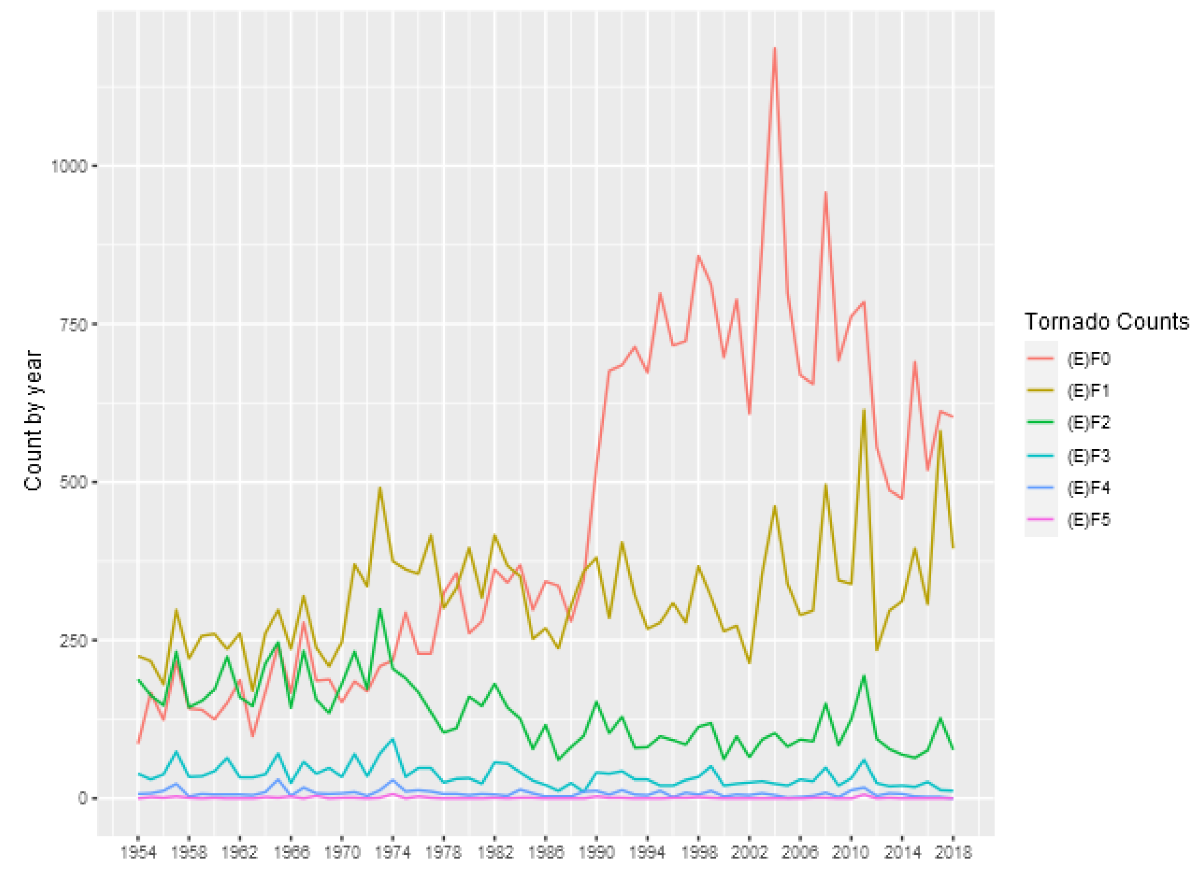
We used in this work a subset of the Storm Prediction Center’s Severe Weather Database file, available at https://www.spc.noaa.gov/wcm/. Although the database covers the 1950–2018 period, we propose to use the 1954–2018 period in order to remove the undercount of tornadoes in the first years, as discussed by Agee and Childs (2014). To facilitate the visualization of the results, we use a yearly aggregation of the daily data. The database also includes damage rating scales, Fujita (F)-prior to 2007- and Enhanced Fujita (EF)-beginning in 2007. Both scales range from 0 (lowest damage indicator) to 5 (highest damage indicator). Table 1 shows some descriptive statistics for the annual counts of tornadoes in each category, and Figure 1 show the number of tornado occurrences reported in each year and each intensity.
In this figure it is possible to observe an increasing in the number of (E)F0 tornadoes after 1990, which can be related to non-meteorological factor Moore (2017). On the other hand, (E)F1 and stronger tornadoes appear to be are stationary. In addition, it is possible to observe a slightly decreasing in the number of (E)F1 and (E)F2 tornadoes after 1974, which can be related to changes in tornado intensity classification adopted by National Weather Service, as discussed by Moore (2017). The occurrences of (E)F5 tornadoes are extremely rare, as can be seen in Table 1, therefore, hereafter we just consider (E)F4 and weaker tornadoes.
3. Results
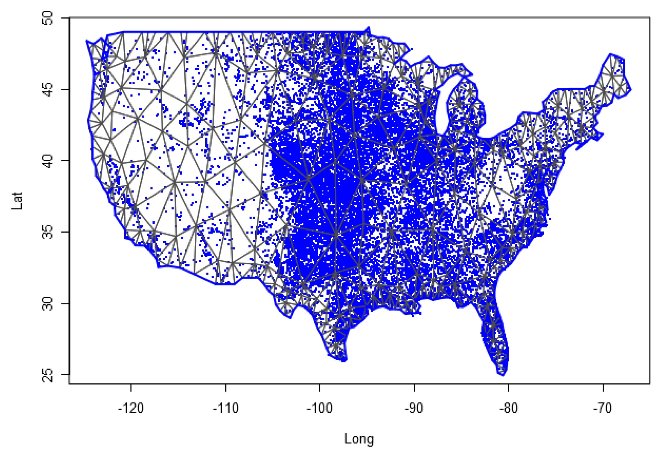
To apply the inference procedures discussed in Section 2, the first step is to define a triangulation mesh of the interest region. Here, we define a triangulation mesh with 439 triangles covering all the United States area. Figure 2 shows the spatial mesh used in the work, and as an illustration we put dots showing the occurrence of (E)F0 tornadoes for the entire sample used. A discussion of criteria for choosing mesh size in estimating LGCP models can be found in Simpson et al. (2016). As discussed in this work, the use of the continuous approximation for LGCP avoids the use of very thin meshes in the process approximation, and thus allows representing and estimate the parameters and random effects in a computationally efficient way. This characteristic is especially important in space-time models, where the computational representation of the process is very intensive in memory.
The second step is to define a set of knots over time to build a temporal mesh. For the time domain, we define a temporal mesh based on the number of observed years, 65. To obtain the space-time aggregation, we find to which polygon belongs each data point in the spatial mesh and to which part of the time belongs each data point. Hereafter, we use these both identification index sets to aggregate the data.
As described in Equation (1), we estimate the parameters associated with the dynamic and spatial components. The parameters are the intercept (), the precision of the trend component () and cycle component (). The parameters of the second-order autoregressive process of the cycle are parameterized as partial autocorrelations (PACF1 and PACF2), whereas the parameters of spatial covariance are represented by and and the parameter of spatial time dependence (). As previously discussed, in this work we use the estimation structure based on Integrated Nested Laplace Approximations (INLA) to estimate the parameters and random effects of the model. For reasons of space, we do not detail these procedures, and we indicate Rue et al. (2009) for the INLA method and the details of SPDE approximation for LGCP can be found in Simpson et al. (2016).
In Table 2 we present the estimated posterior distribution for the parameters associated with the model given by Equation (1), for the tornado classifications (E)F0-(E)F4. The intercept parameter estimates the unconditional mean of the estimated log intensity function, and we can see that the values are consistent with the observed magnitude of the number of tornadoes in each classification. The precision parameters report the variability associated with the trend and cycle processes. Greater precision is associated with less variability in the component, and again the results are consistent with the general patterns of the number of tornadoes occurring in each category analyzed. The partial correlation parameters are related to the autoregressive parameters in the AR (2) representation of the cycle. In all estimates, the results indicate the presence of a cyclic component, since the roots of the lag polynomial associated with the estimated partial correlation coefficients fall in the complex region. The estimated period for the cycle components for (E)F0, (E)F1, (E)F2, (E)F3 and (E)F4 tornadoes are, respectively, 3.98, 5.63, 5.59, 2.78, and 3.09 years. These periods are consistent with those observed for climatic phenomena associated with interactions between sea temperature and the atmosphere, such as El Niño and La Niña (ENSO), as discussed in Cook et al. (2017). Please note that the interpretation of this cycle component is an approximation for the effects of all shocks with persistent but non-permanent effects that affect the occurrence of tornadoes.
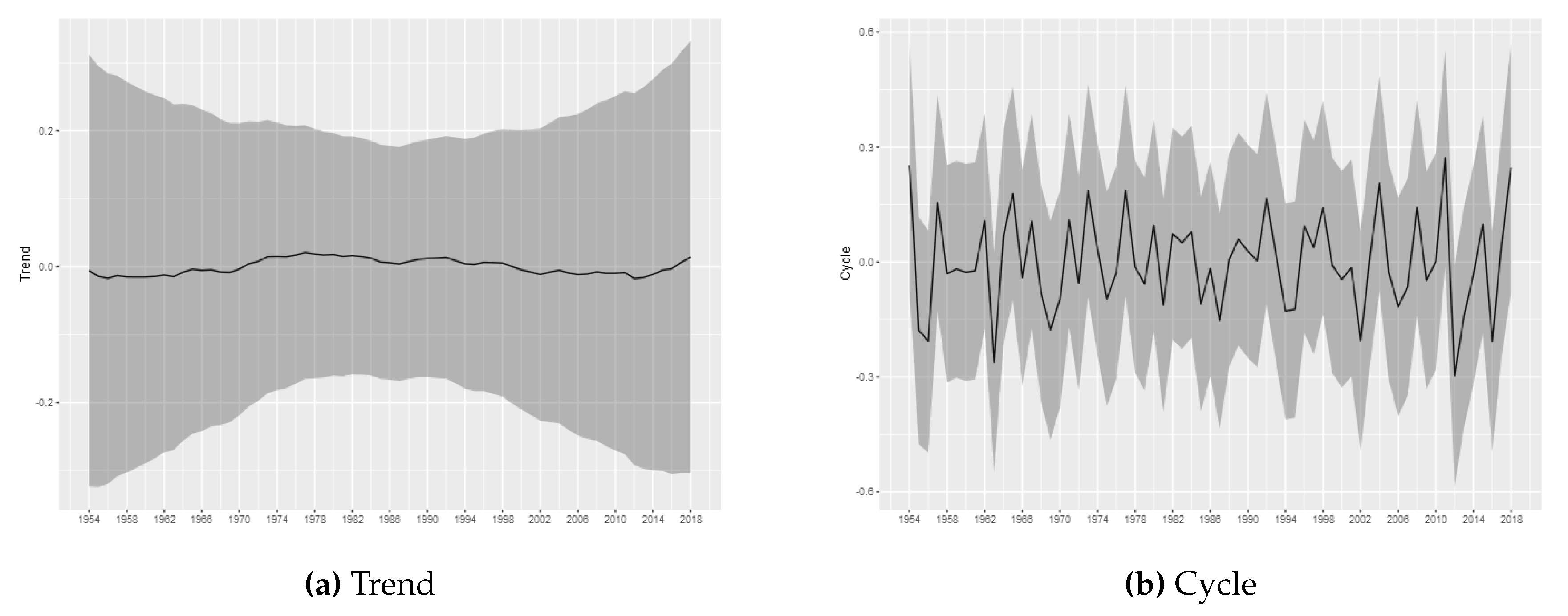
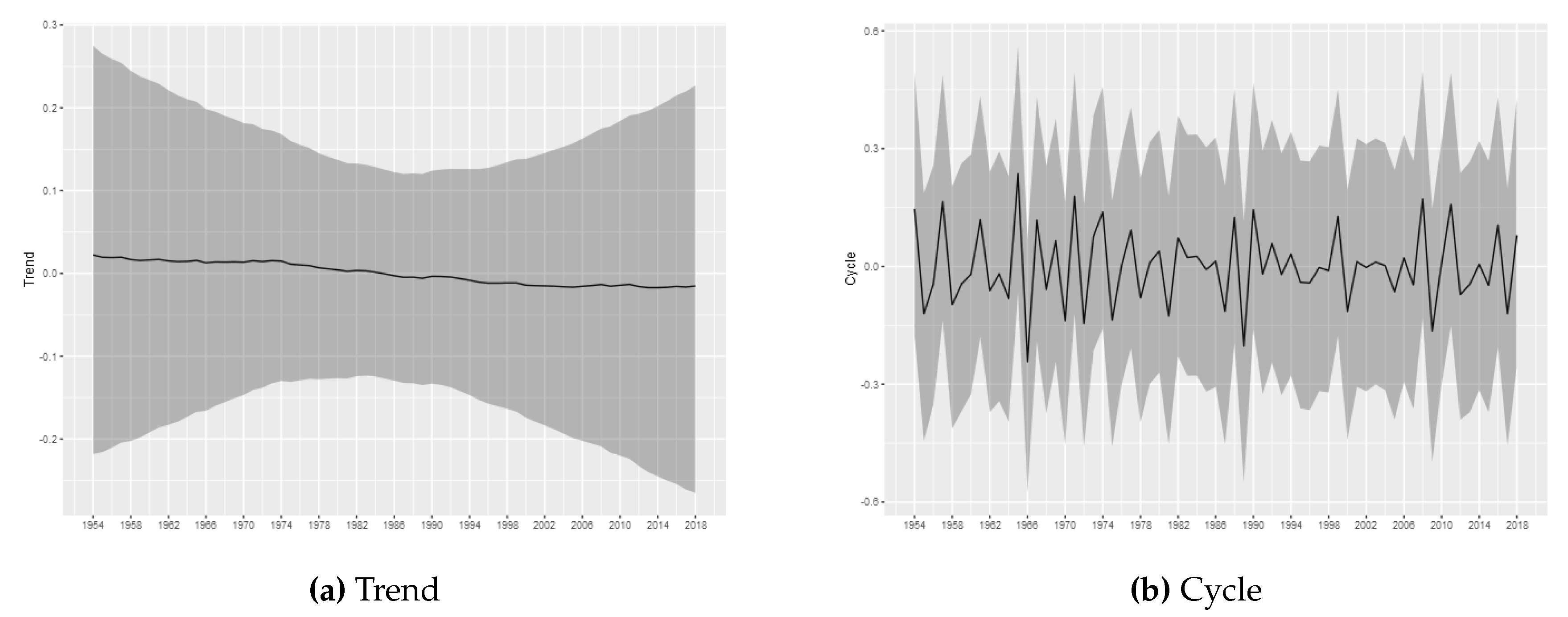
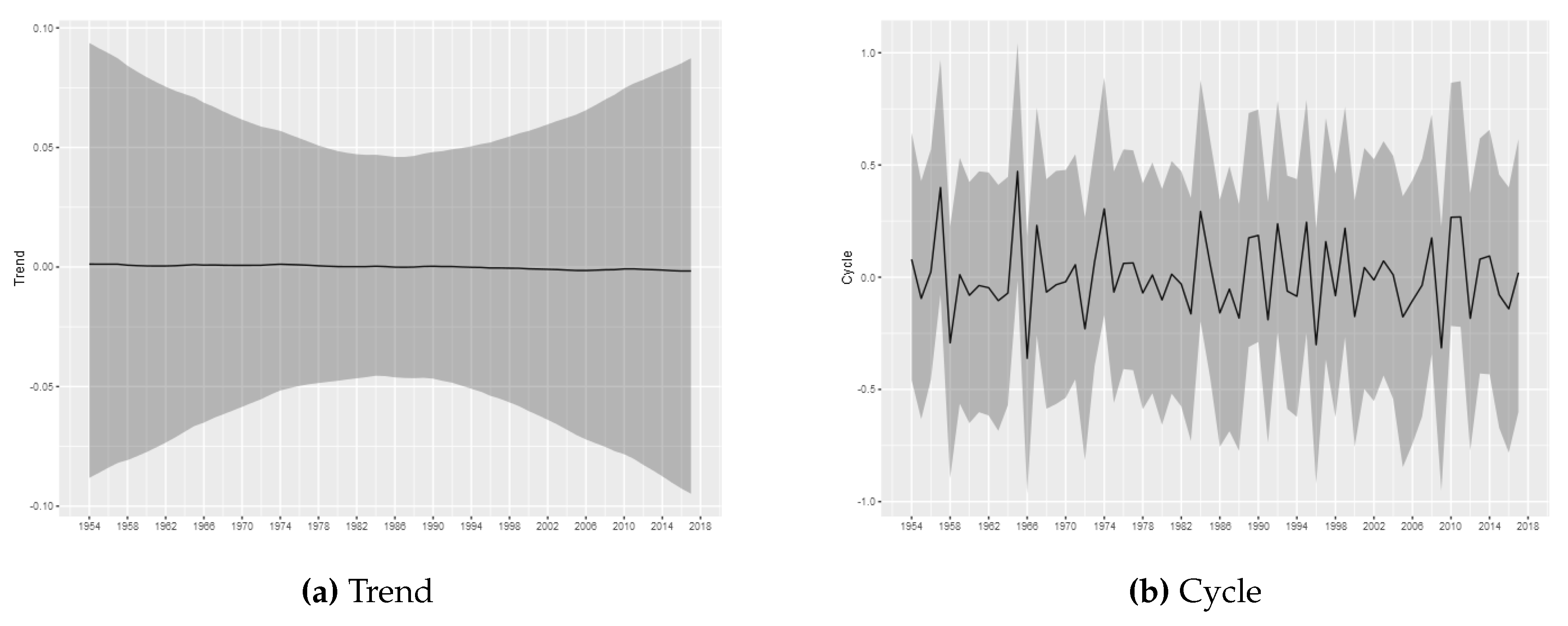
The estimated trend and cycle components for each tornado log intensity are shown in Figure 3, Figure 4, Figure 5, Figure 6 and Figure 7, which present the posterior mean of the estimated components with 95% Bayesian credibility interval. The most important result is related to the trend component. Considering (E)F0 tornadoes, it is possible to observe a growth pattern in the trend component between 1962 and 2000, whereas between 2000 and 2016 it remains stable. From 2016 can be seen a growth pattern again. This result is consistent to results commonly found in the literature and, as discussed by Moore (2017), part of this effect can also be attributed to non-meteorological factors such as changes in reporting practices, reporting procedures, and observing technology. As argued by Brooks and Doswell III (2001), information about tornadoes comes from untrained witnesses, which may have led to basic errors in reporting practice. Weaker tornadoes are likely to be missed in the reporting since they have short lifetimes and path lengths, while stronger tornadoes may be more reliably reported (Brooks and Doswell III 2001; Kunkel et al. 2013; Verbout et al. 2006). An additional component of the increase trend in the F0 tornadoes is likely due to the policy change in 1982 which have established that all tornadoes that did not have rated damage must be classified as (E)F0 (Brooks 2004). Despite the evidence that the (E)F0 series may increases due to non-meteorological factors, it is important to note that our proposed model is able to capture the effects of exogenous changes and may capture possible changes in the spatial distribution, even if the trend is not associated with climate changes.
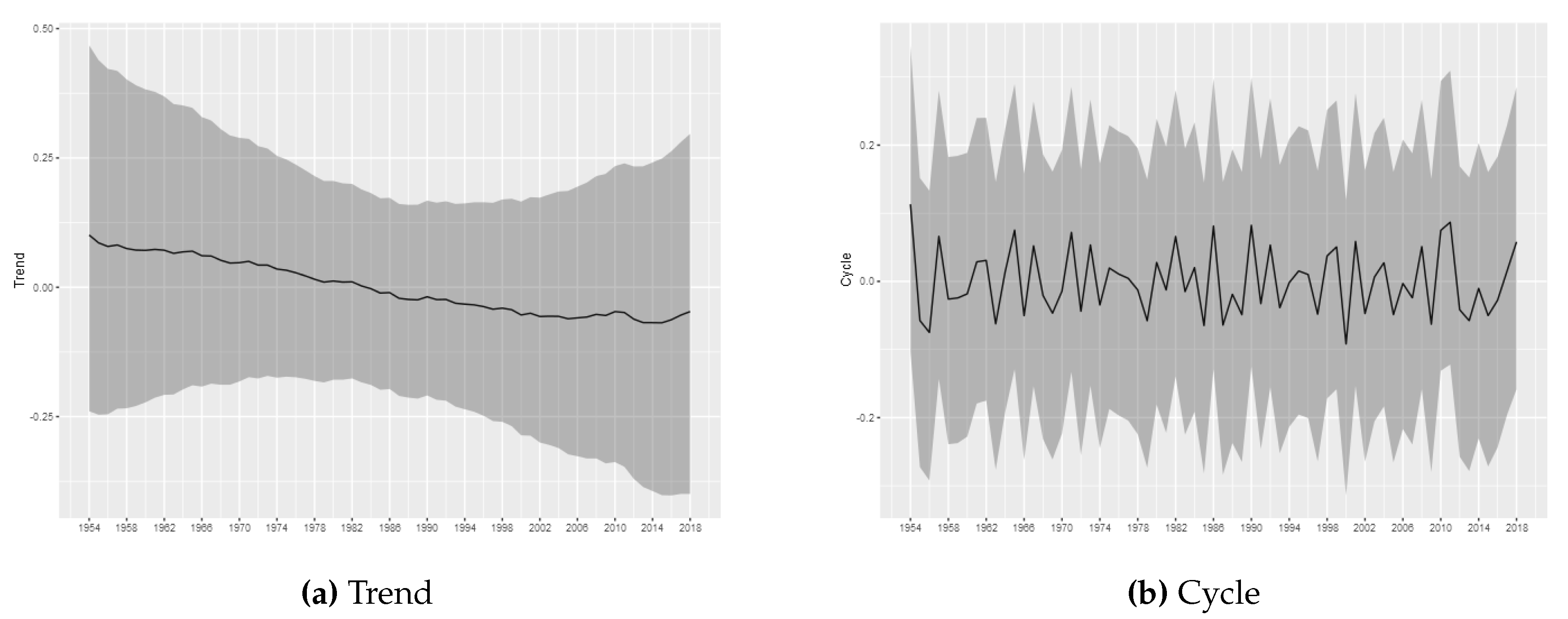
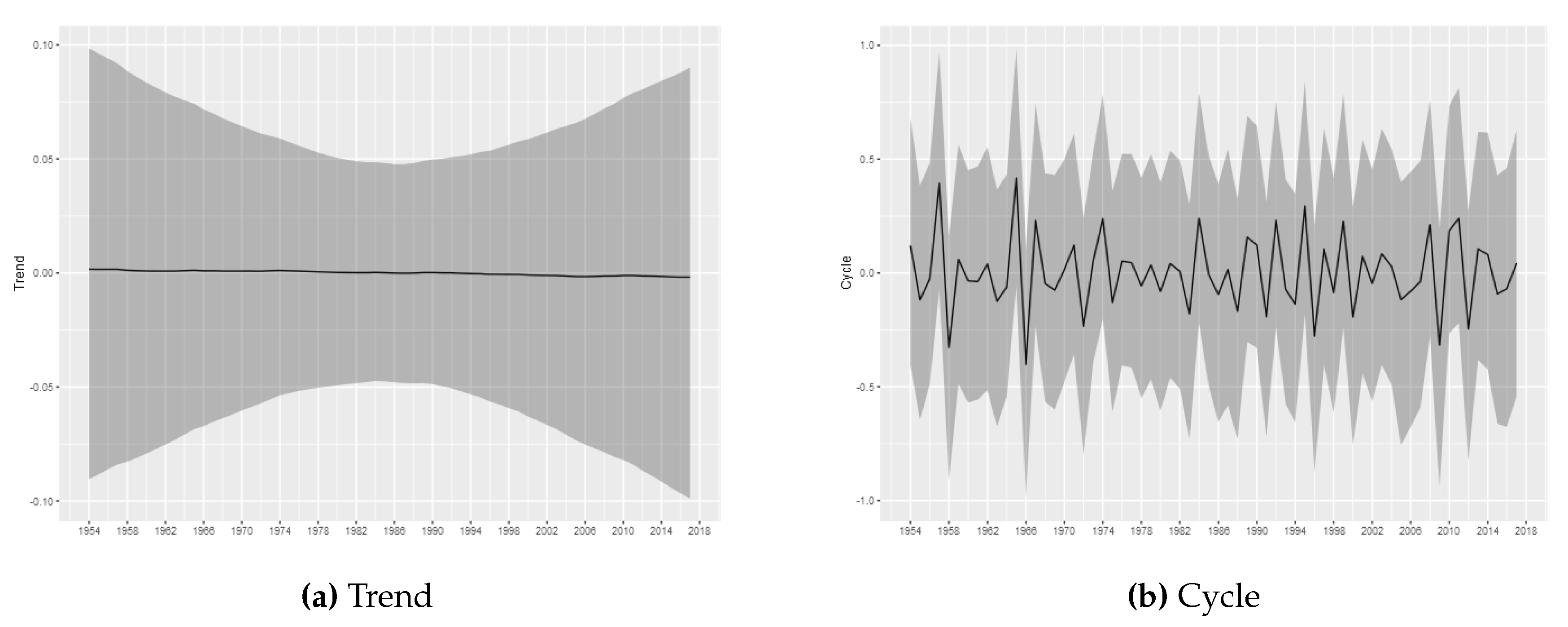
For the tornadoes of (E)F1-(E)F4 classification, it is not possible to infer permanent changes in the occurrence intensity. The estimated trend components do not show relevant variations, being all estimated close to zero, with the credibility intervals always covering this value. The results obtained through the modeling carried out in this article do not indicate the presence of relevant changes in the trend of occurrences for these categories of tornadoes. Considering (E)F1-(E)F4 tornadoes, the results are consistent with stationary patterns in the temporal counts of tornado occurrences, in line with the results found in Kunkel et al. (2013) and Moore (2017).
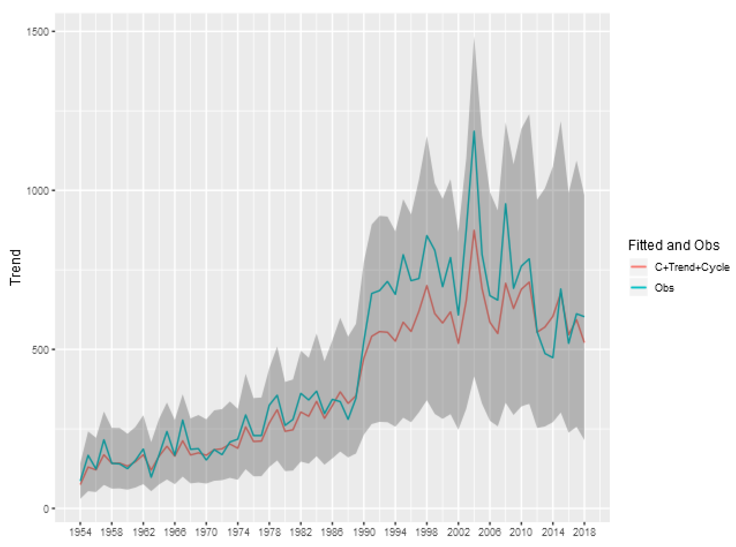
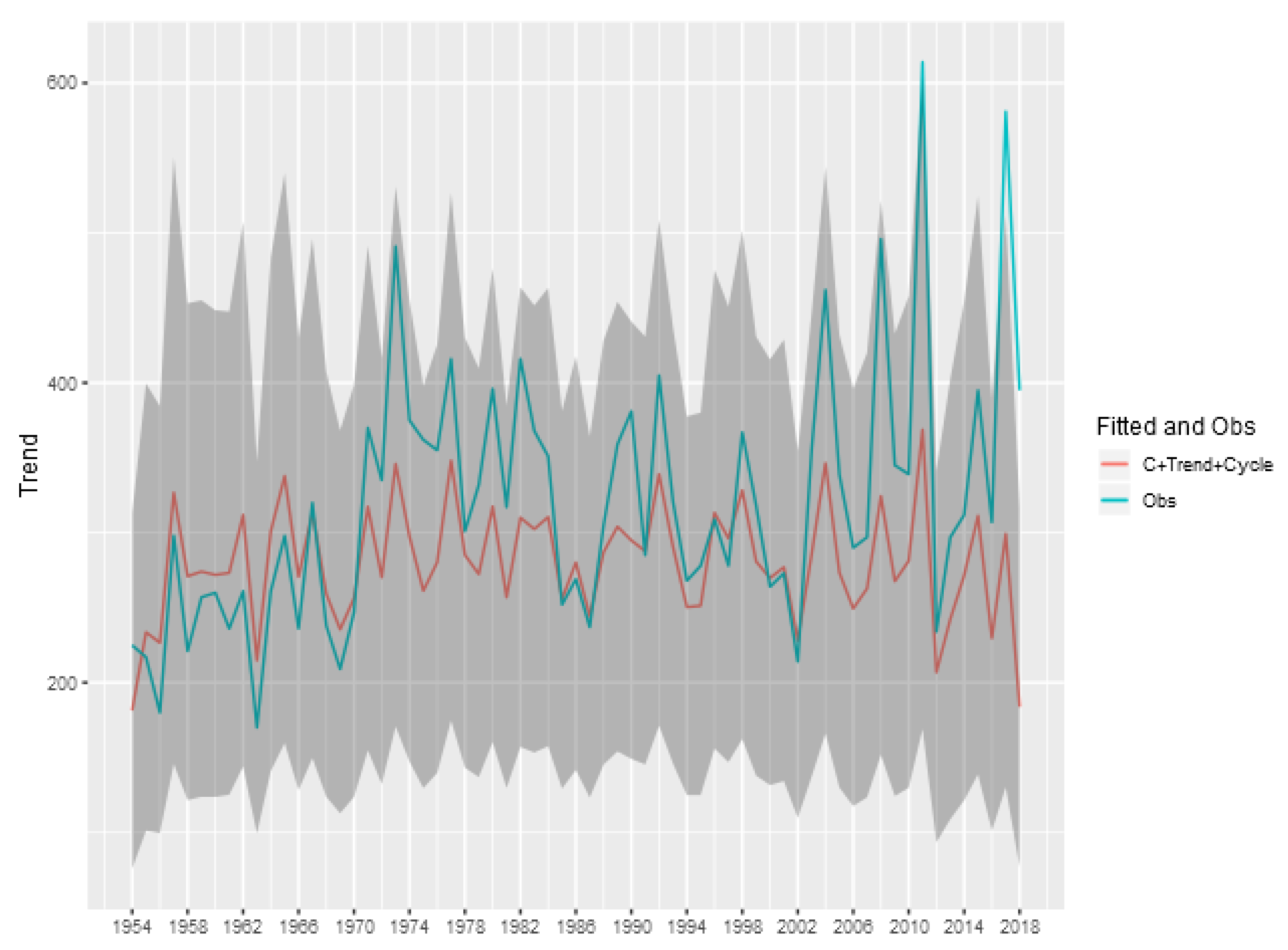
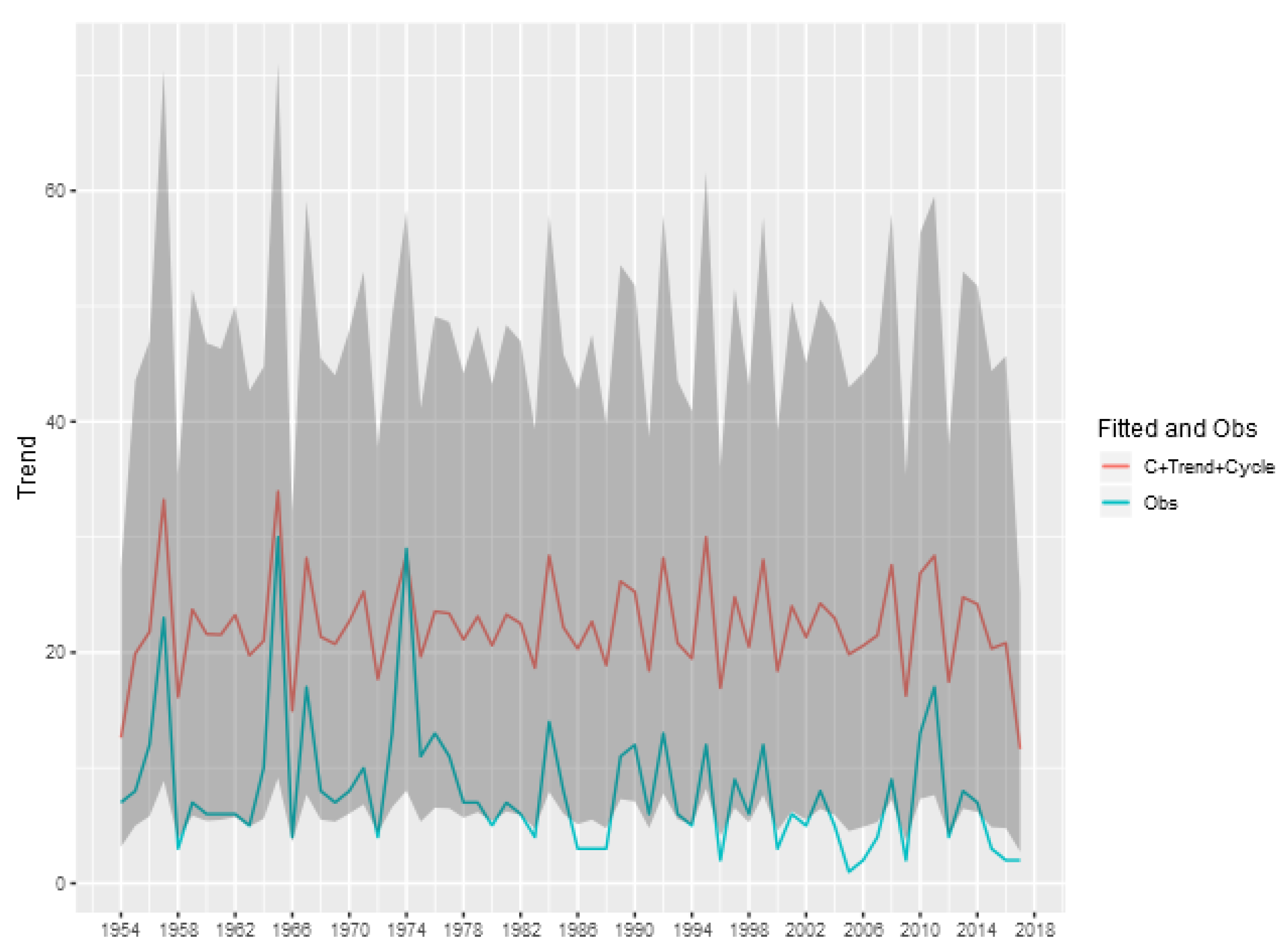
To show the importance of the trend and cycle components in the analysis of the tornado occurrence patterns, we show in Figure 8 the predicted value for the tornado count (E)F0 in each year given by the sum of the trend, cycle and intercept components of model, and also the credibility interval of this sum. This represents the prediction of the total count ignoring the spatial random effect, obtained by aggregating the exposure of the entire area multiplied by the exponential of the sum of these components. The analogous figures for the other classifications (Figure A1, Figure A2, Figure A3 and Figure A4) are shown in the Appendix of the article.
We can see that for the (E)F0 and (E)F1 classifications, the random effects of trend and cycle explain a large part of the variability observed in the total tornado count. For the other classifications, the spatial component is more relevant in explaining the count observed each year, indicating a greater spatial heterogeneity in the intensity of occurrences.
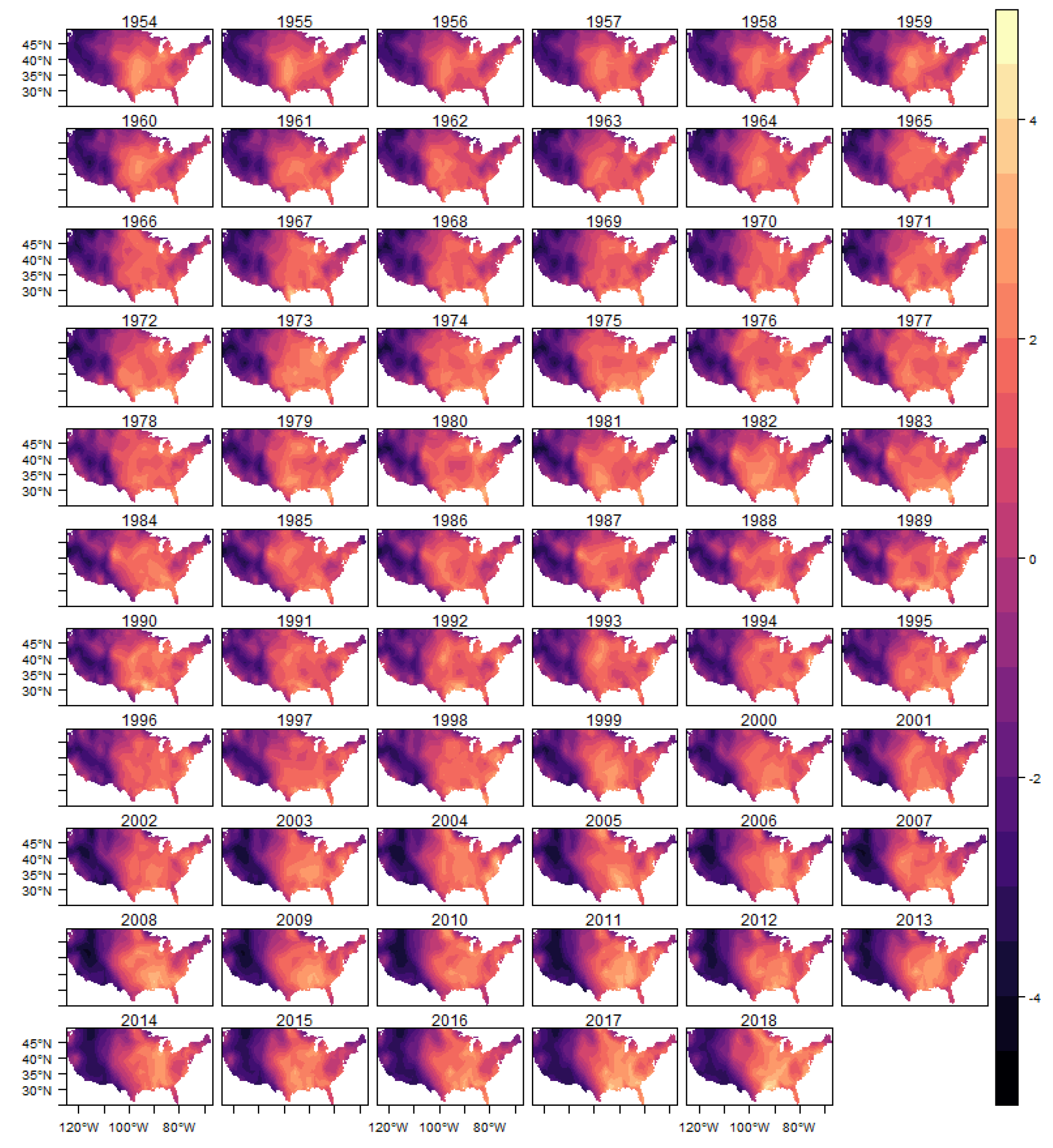
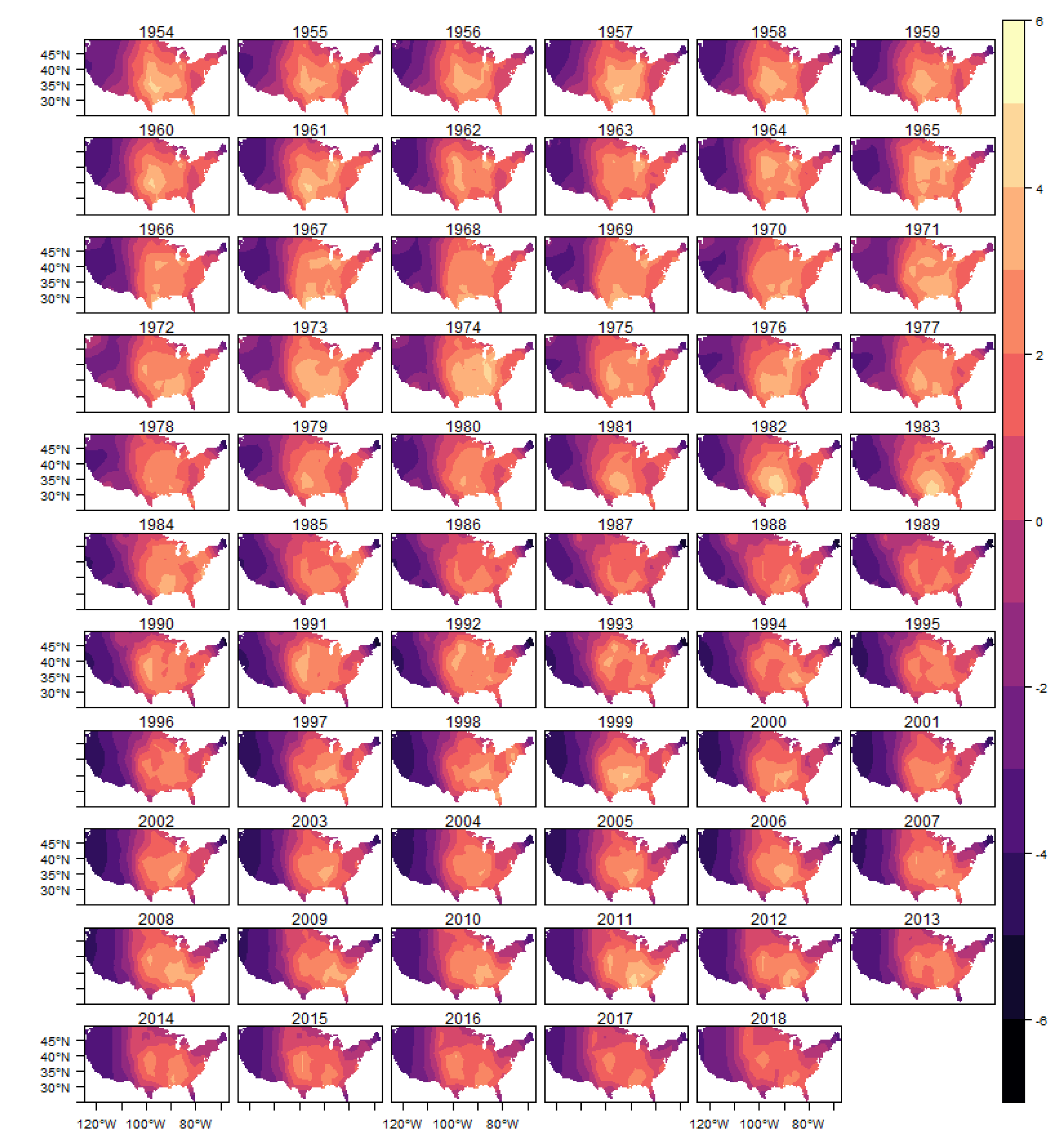
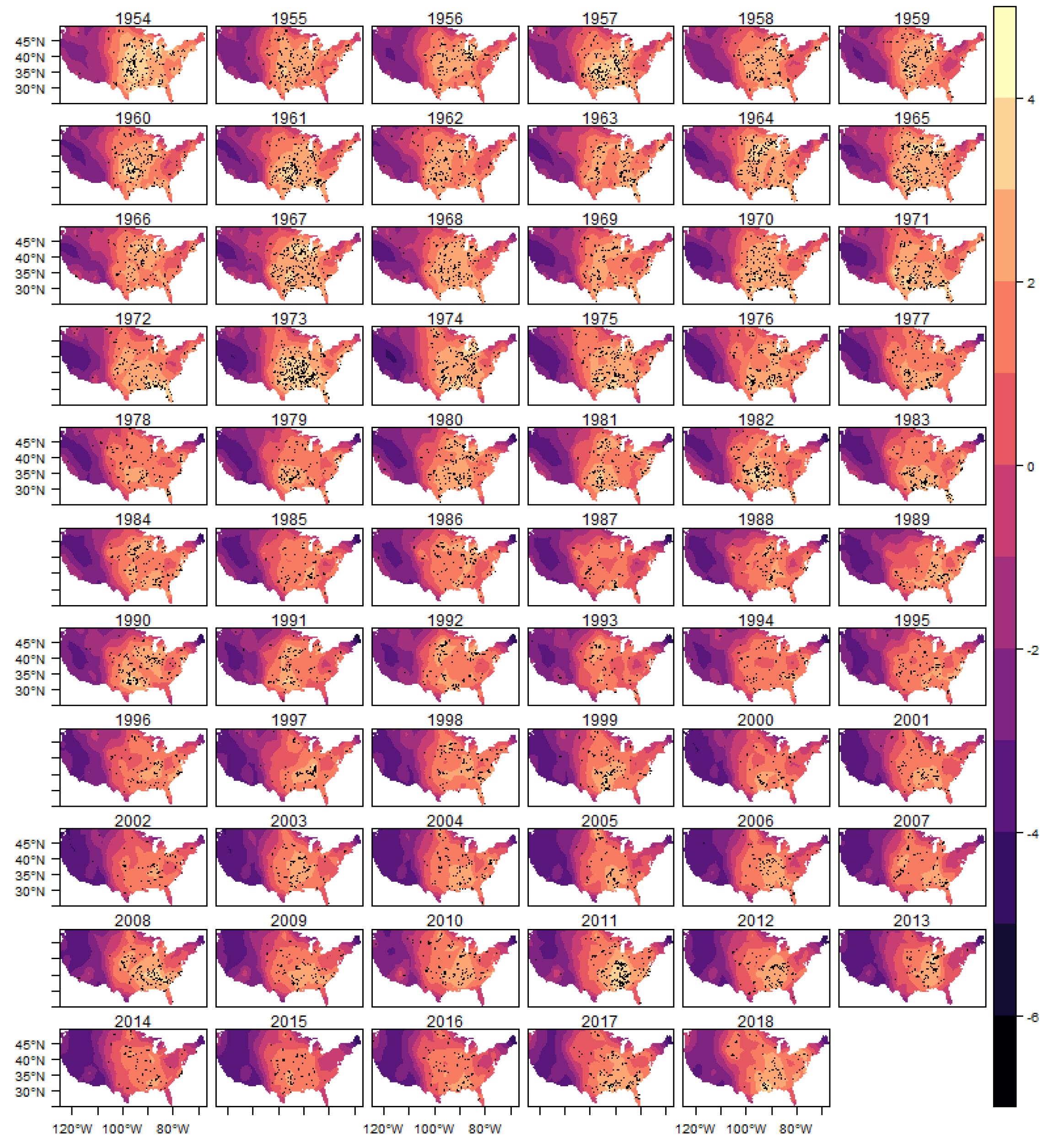
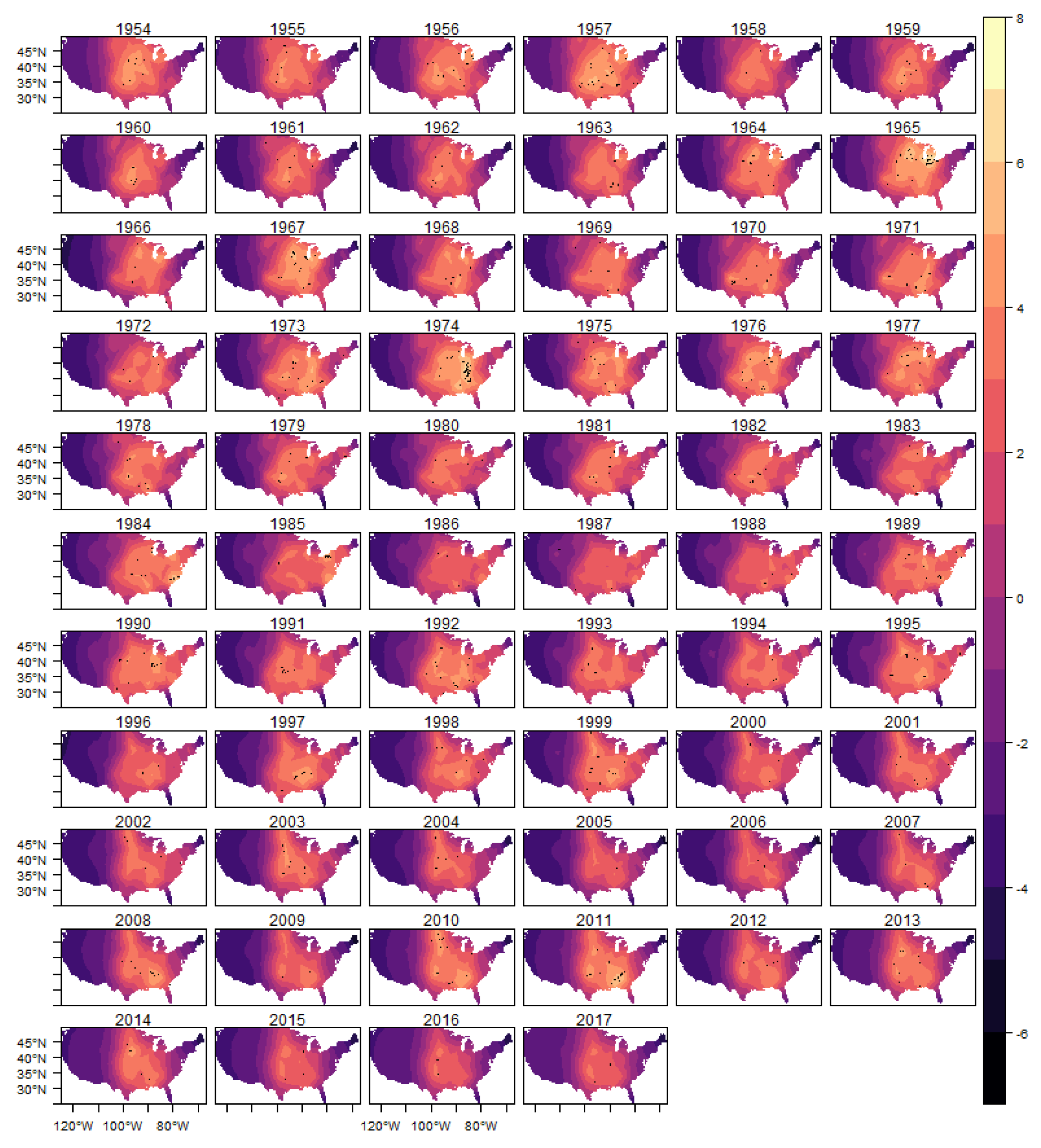
The spatial heterogeneity of the tornado occurrences can be seen through the estimated spatial random effect . In this section, we show in Figure 9 the estimated posterior distribution of spatial random effect for (E)F0 tornadoes, and in the appendix of the article the results for the other classifications in Figure A5, Figure A6, Figure A7 and Figure A8.
In these figures it is possible to observe the variability captured by the spatial random effects, especially in the region known as Tornado Alley, which is a nickname given to an area in the southern plains of the central United States that experiences a high frequency of tornadoes each year (NOAA). In addition, after 1980s, it is also possible to observe an increasing in the variability in the Southeast region, for all intensities considered, which is consistent with finds reported in the literature (e.g., Moore and DeBoer (2019) and Gensini and Brooks (2018)).
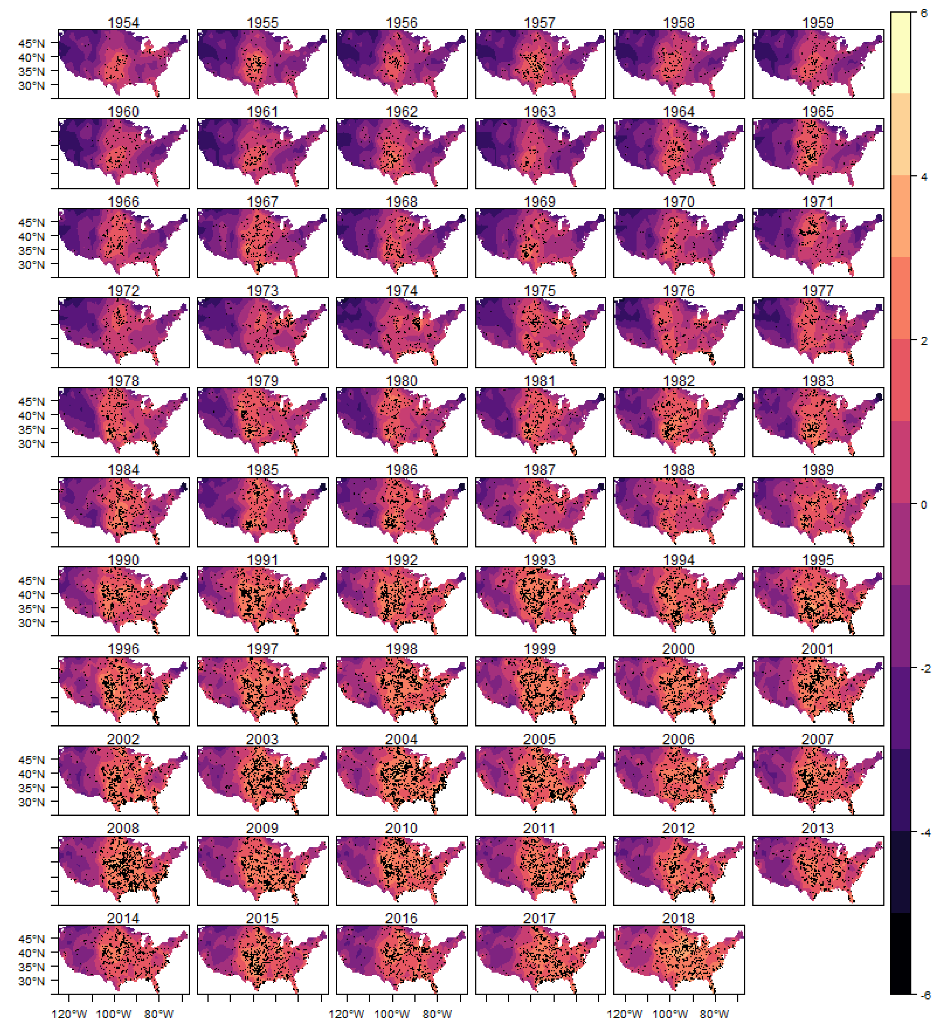
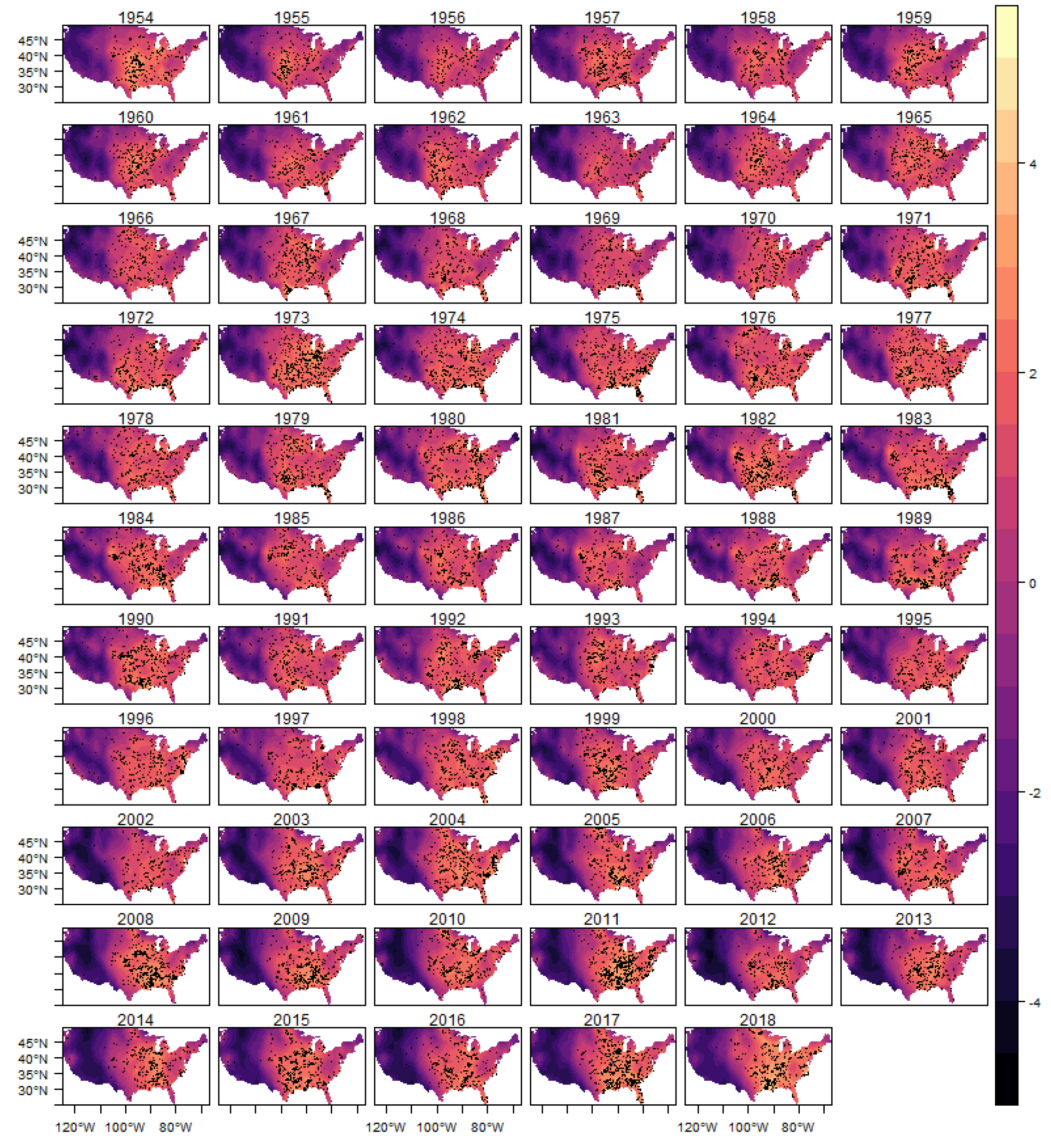
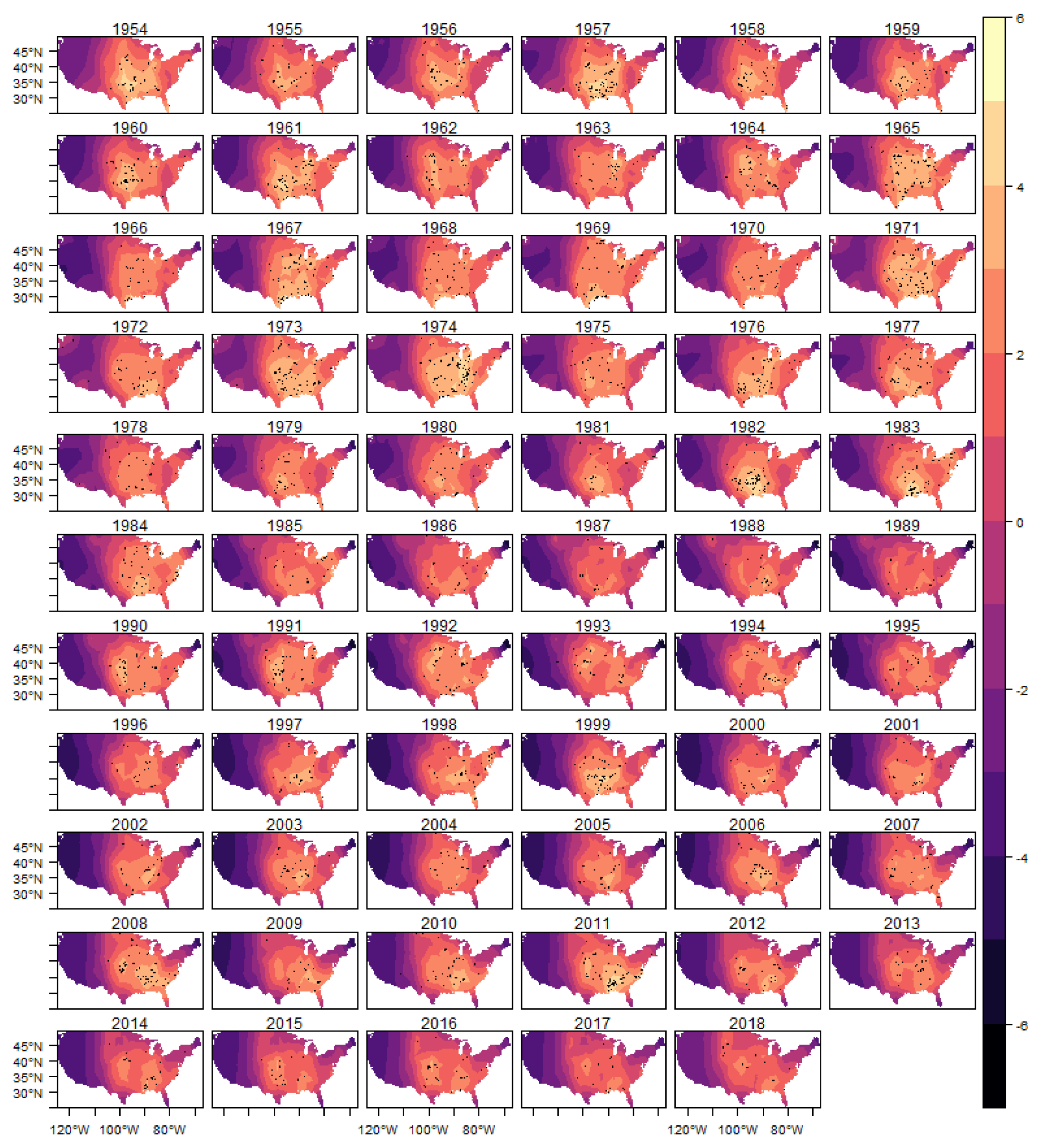
In Figure 10 we show the estimated intensity function for the (E)F0 classification tornadoes, given by the sum of all random components (trend, cycle and spatial) in each year. The analogous results for the other classifications are shown in Figure A9, Figure A10, Figure A11 and Figure A12 in the Appendix.
In each year presented in these figures we also show the observed occurrences of tornadoes as black dots. We can observe that the estimated intensity log function adequately explains the spatio-temporal variation observed in the tornado count for all classifications, indicating that the space-time LGCP model proposed in this work has an adequate fit to the analyzed pattern of occurrences.
To verify the robustness of the results found and the importance of the estimated components, we analyzed different specifications of the model using information criteria. We compared for each classification of tornadoes four restricted versions of the model. Table 3 shows the Deviance information criterion (DIC), a generalization of the Akaike information criterion proposed in Spiegelhalter et al. (2010) and the widely applicable information criterion (WAIC), also known as Watanabe–Akaike information criterion, another generalization of the Akaike information criterion, proposed in Watanabe (2010) and Watanabe (2013).
Model M0 in Table 3 corresponds to the model with trend, cycle, and the time varying spatial random effects. The first restricted specification (M1) assumes that there is no trend component, and so there is no permanent change in the long-term average pattern for tornadoes. The second specification (M2) assumes the restriction that there is no cycle component and including the trend and time varying spatial random effects, the third specification (M3) assumes that the spatial random effects are constant over time, but including the trend and cycle components. The last specification (M4) assumes only an intercept and fixed spatial random effects.
Thus, these different specifications allow to analyze the impact of each component of the model on the spatio-temporal dynamics of tornadoes. The restricted specifications are important for the analysis of possible climate changes, since they analyze changes in long-term permanent patterns (trend) and possible changes in the spatial distribution of tornadoes over time.
In Table 3 the best specification for each classification is marked in bold. For the (E)F0 classification, the DIC points out as the best specification M1, which includes trend, cycle and time-varying spatial effects, and WAIC selects the M2. For the (E)F1 classification the best specification is M2 by both
criteria, suggesting that for this classification the cycle effects are not relevant for the explanation of
the tornado pattern, a result consistent with the estimated magnitude of the cycles shown in Figure 4,
and consistent with the patterns of change in the trend and the spatial component over time.
For the (E)F2 classification, the M1 model is selected by the DIC criterion, while for WAIC the M2 is selected, indicating the importance of the temporal variation pattern in the spatial component, and doubt about the inclusion of the trend. The model selected by the DIC is consistent with the results shown in Figure 6, which indicate little variability in the trend. The results for the (E)F4 classification are substantially different, selecting the M3 model, which includes the trend and cycle components, but assumes that the spatial random effects are fixed in time. The absence of relevant variations in the spatial component is consistent with the results shown in Figure A8. It is important to note that the lower number of occurrences in this class of tornadoes makes the identification of variations in temporal patterns less accurate. The parameters estimated in these specifications and other results are available under request from the authors.
Other alternative specifications were also tested in relation to the mesh size used, the numerical method to determine the modes in the Laplace approach and methods for the numerical integration. The results are qualitatively invariant when choosing the mesh size, and we used a mesh size that was computationally efficient in terms of memory usage and processing speed, which are especially important when comparing models. Thinner mesh construction did not produce more accurate or qualitatively different results. It is not possible to show a comparison of information criteria in this case since different mesh sizes are not directly comparable in terms of model fit, as they have different sample sizes.
Different methods of numerical optimization found the same results (modes) in the Laplace approximation. We analyzed four alternatives in the Laplace approximations. The first three forms, described in Rue et al. (2009), are the Gaussian, simplified and full Laplace approximations, and last form is the adaptive method, described in Gomez-Rubio (2020), which is computationally more efficient at the cost of greater memory usage. The results are basically the same in all approximation methods. The construction of the precision matrices (reordering) and the sparse linear algebra tools use the paradiso library which allows a great gain in numerical efficiency.
It is important to discuss some limitations of this study. A relevant point is related to model identification, given the high persistence of the autoregressive parameter of spatial random effect. To avoid a possible identification problem, we impose that the autoregressive term is time stationary in the estimation of the spatial random effect through a transformation, representing the parameter as . For finite values of this minimizes the identification problems generated by a unit root in this coefficient and the simultaneous inclusion of the trend. However, it is still possible that the value of the autoregressive coefficient is very close to one. An alternative may be to investigate a model with several common trends. However, this is not possible yet, because there are some important limitations that must be circumvented. One of these limitations is that our structure of spatial random effects is continuous in the space. Thus, there is not a straightforward way to determine what regions of the continuum would be affected by each trend in the model. In the limit we must have a coefficient that is a continuous function in the space, which has not yet been done for this class of models. To avoid this problem, an alternative would be to discretize the space and impose that each discretized region has a separated trend. The problem is that this alternative involves ad-hoc choices, since to the limit of our knowledge, there is no method developed for this problem. Another alternative may be assuming that the spatial effect is a random walk process. In this case, each location in the continuum would have a particular trend. Nonetheless, in this case, the problem would be the non-stationarity.
In this case, one may consider the use of nonstationary spatial modelling with explanatory variables in the dependence structure, as described by Ingebrigtsen et al. (2014), which have proposed a flexible class of non-stationary models where explanatory variables can be easily included in the dependence structure. In this specification, the covariance parameters are determined through a log-linear regression with coefficients for possible explanatory variables defined on the mesh, allowing that these coefficients spatially vary. The difficulty of this specification in the tornado modelling is due the fact that the spatial variation of tornadoes depends on air mass movements, which have a great seasonal variation, which makes this method substantially difficult to implement. The application of this methodology including fixed covariates, such as latitude, longitude, distance to coast and elevation would be considered for future papers.
Zero-Inflated Poisson
Data were taken for different intensities of tornadoes, based on Fujita (F) and Enhanced Fujita (EF) damage rating scales. Historically, stronger tornadoes are less likely to occur, which led to the database having many zero counts. For classifications with very few occurrences, a possible modification is to change the likelihood function to account for the possibility of an excess of zeros. Mixed-distribution models, such as Zero-Inflated-Poisson (ZIP) can be used in such cases. According to Lambert (1992), ZIP is a model for count with excess zeros, which assumes that with probability p the observation is 0, and with probability , a Poisson is observed.
We consider two different types of ZIP models: type 0 and type 1. The type 0 likelihood is defined as
where p is a hyperparameter where
and is the internal representation of p, meaning that the initial value and prior is given by . On the other hand, the type 1 is defined as
where p is a hyperparameter where
where has the same meaning above-mentioned. As discussed by Serra et al. (2014), the only difference between type 0 and 1 is the conditioning on for type 0, which means that for type 0 the probability that y is equal 0 is p, whereas for type 1, the same probability is .
Table 4 shows the estimated posterior distribution for the parameters associated with the ZIP model for (E)F4 tornadoes, considering type 1. For space issue we show only the results obtained with type 1, which had best results, in terms of fit, in relation to type 0. The results obtained with type 0 are available with the authors. As in Table 2, the precision parameters represent the variability associated with trend and cycle components. The results indicate great precision associated with the trend component whereas the precision of cycle component is relatively minor.
Figure 11 shows the estimated trend and cycle components for the (E)F4 tornadoes, considering the ZIP model with type 1, where it is possible to observe the absence of permanent changes in the occurrence intensity. In addition, it is important to note that the ZIP model with type 1 results do not present significant changes in the trend and cycle components, relatively to those results obtained with Poisson distribution and shown in Figure 4, Figure 5, Figure 6 and Figure 7.
4. Conclusions
Climate changes, associated with natural or human activities, can lead to changes in the likelihood of the occurrences of severe weather events, such as heat waves, droughts, tornadoes and hurricanes. The Unites States experiences more tornadoes per year than any other country, which are responsible for deaths and damages. Given the impact of tornadoes on society, understanding how these events are responding to climate changes is important in order to be prepared. Previous studies have searched for relationships between tornado activity and climate changes, for example Lee (2012); Diffenbaugh et al. (2013) and Moore and McGuire (2019).
This present paper contributes to this literature by analyzing tornado occurrences in the United States extending the method proposed by Laurini (2019) using the LGCP representation proposed by Simpson et al. (2016). Therefore, to perform inference procedures for the spatio-temporal point process we adopt a dynamic representation of Log-Gaussian Cox Process. This representation is based on the decomposition of intensity function in components of trend, cycles, and spatial effects. In this model, spatial effects are also represented by a dynamic functional structure, which allows analyzing the possible change in the spatial distribution.
The decomposition proposed in this article is therefore especially useful when analyzing possible changes in the temporal and spatial patterns of the occurrence of events, since it captures changes in the average number of occurrences through the trend component, and changes in the spatial distribution pattern through the time varying spatial random effect. We use daily data from Storm Prediction Center’s Severe Weather Database between 1954 and 2018. The results have provided evidence, from new perspectives, that trends in annual tornado occurrences in the United States have remained relatively constant, supporting previously reported findings.
Author Contributions
F.V. and M.L. share equally in all aspects of the paper: Conceptualization; methodology; software; validation; formal analysis; investigation; resources; data curation; writing–original draft preparation; writing–review and editing; visualization; project administration. All authors have read and agreed to the published version of the manuscript.
Funding
The authors acknowledge funding from CNPq (306023/2018-0) and FAPESP (2018/04654-9). This study was financed in part by the Coordenação de Aperfeiçoamento de Pessoal de Nível Superior (CAPES)-Finance Code 001 and Instituto Escolhas.
Conflicts of Interest
The authors declare no conflict of interest.
Appendix A. Fitted and Observed Tornadoes without Spatial Component
Figure A1.
Fitted and Observed Tornadoes without consider the spatial effects-(E)F1.

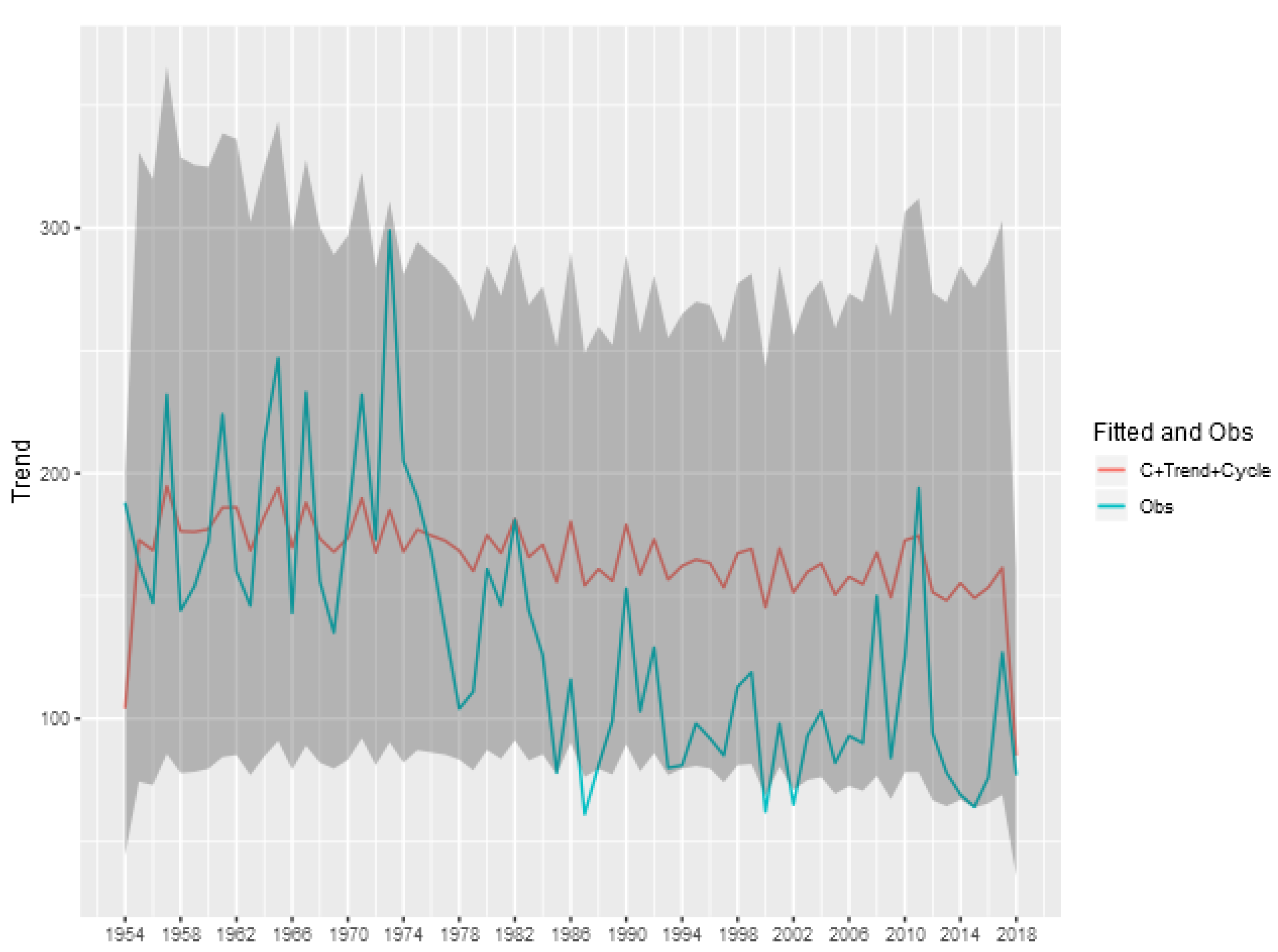
Figure A2.
Fitted and Observed Tornadoes without consider the spatial effects-(E)F2.

Figure A3.
Fitted and Observed Tornadoes without consider the spatial effects-(E)F3.

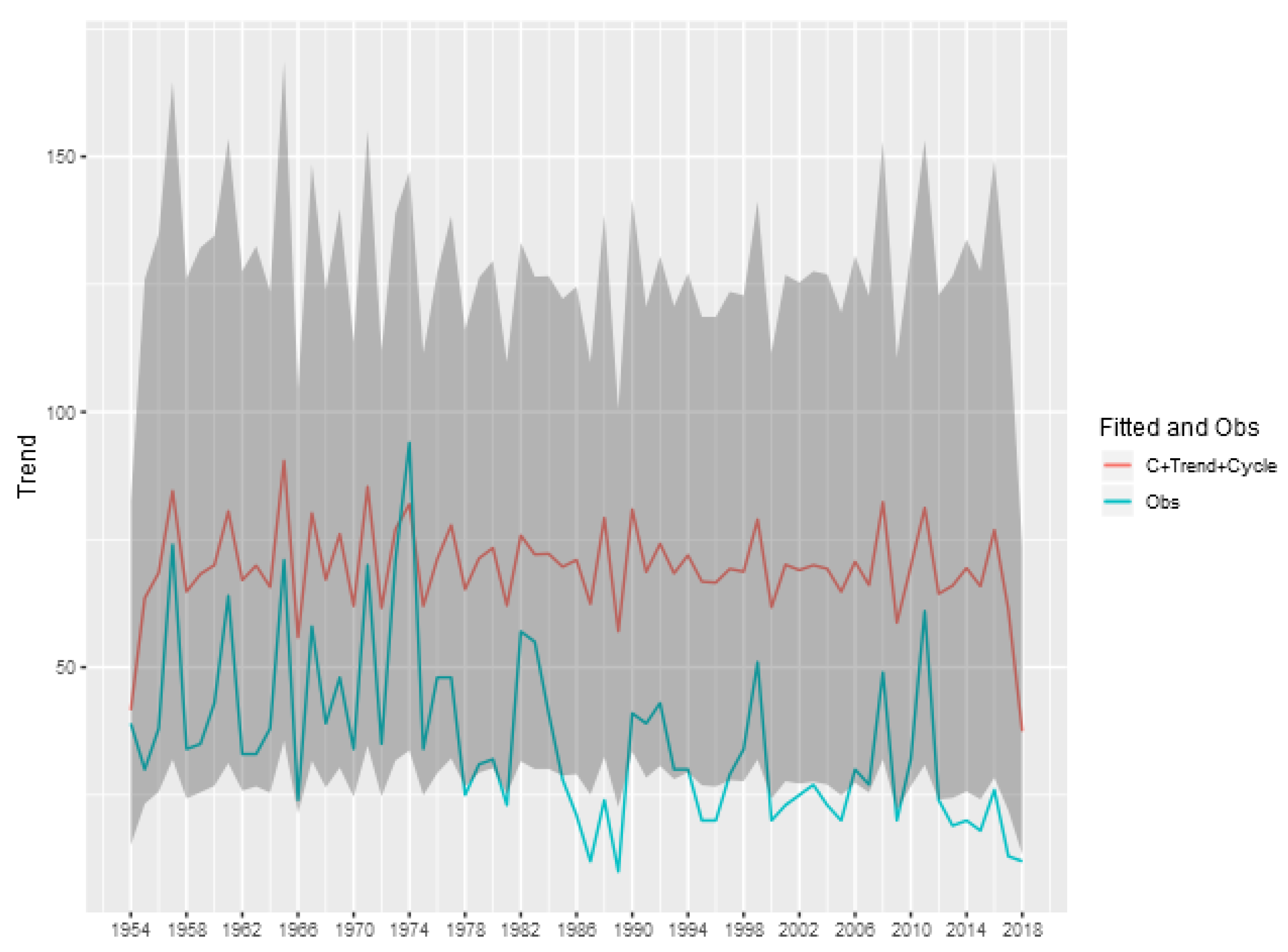
Figure A4.
Fitted and Observed Tornadoes without consider the spatial effects-(E)F4.

Appendix B. Spatial Random Effects
Figure A5.
Spatial Random Effects-(E)F1.

Figure A6.
Spatial Random Effects-(E)F2.

Figure A7.
Spatial Random Effects-(E)F3.

Figure A8.
Spatial Random Effects-(E)F4.

Appendix C. Fitted Log-Intensity and Observed Tornadoes
Figure A9.
Fitted Log-Intensity and Observed Tornadoes-(E)F1.

Figure A10.
Fitted Log-Intensity and Observed Tornadoes-(E)F2.

Figure A11.
Fitted Log-Intensity and Observed Tornadoes-(E)F3.

Figure A12.
Fitted Log-Intensity and Observed Tornadoes-(E)F4.

References
- Agee, Ernest, and Samuel Childs. 2014. Adjustments in tornado counts, f-scale intensity, and path width for assessing significant tornado destruction. Journal of Applied Meteorology and Climatology 53: 1494–1505. [Google Scholar] [CrossRef]
- Allen, Myles R., Vicente R. Barros, John Broome, Wolfgang Cramer, Renate Christ, John A. Church, Leon Clarke, Qin Dahe, Purnamita Dasgupta, Navroz K. Dubash, and et al. 2014. Climate Change 2014 Synthesis Report. Technical Report. Geneva: Intergovernmental Panel on Climate Change (IPCC). [Google Scholar]
- Bakka, Haakon. 2013. How to solve the stochastic partial differential equation that gives a Matérn random field using the finite element method. arXiv arXiv:1803.03765. [Google Scholar]
- Brooks, Harold, and Charles A. Doswell III. 2001. Some aspects of the international climatology of tornadoes by damage classification. Atmospheric Research 56: 191–201. [Google Scholar] [CrossRef] [Green Version]
- Brooks, Harold E. 2004. On the relationship of tornado path length and width to intensity. Weather and Forecasting 19: 310–19. [Google Scholar] [CrossRef] [Green Version]
- Cook, Ashton Robinson, Lance M. Leslie, David B. Parsons, and Joseph T. Schaefer. 2017. The impact of El Niño–Southern oscillation (ENSO) on winter and early spring US tornado outbreaks. Journal of Applied Meteorology and Climatology 56: 2455–78. [Google Scholar] [CrossRef]
- Diffenbaugh, Noah S., Martin Scherer, and Robert J. Trapp. 2013. Robust increases in severe thunderstorm environments in response to greenhouse forcing. Proceedings of the National Academy of Sciences 110: 16361–66. [Google Scholar] [CrossRef] [PubMed] [Green Version]
- Gensini, Vittorio A., and Harold E. Brooks. 2018. Spatial trends in United States tornado frequency. npj Climate and Atmospheric Science 1: 38. [Google Scholar] [CrossRef] [Green Version]
- Gomez-Rubio, Virgilio. 2020. Bayesian Inference with INLA. Boca Raton: Chapman & Hall-CRC. [Google Scholar]
- Harvey, Andrew C. 1989. Forecasting, Structural Time Series and the Kalman Filter. Cambridge: Cambridge University Press. [Google Scholar]
- Illian, Janine B., Sigrunn H. Sørbye, Håvard Rue, and Ditte K. Hendrichsen. 2010. Fitting a Log Gaussian Cox Process with Temporally Varying Effects–A Case Study. Technical Report. Trondheim: Norges Teknisk-Naturvitenskapelige Universitet. [Google Scholar]
- Illian, Janine B., Sigrunn H. Sørbye, and Håvard Rue. 2012. A toolbox for fitting complex spatial point process models using integrated nested Laplace approximation (INLA). Annals of Applied Statistics 6: 1499–530. [Google Scholar] [CrossRef] [Green Version]
- Ingebrigtsen, Rikke, Finn Lindgren, and Ingelin Steinsland. 2014. Spatial models with explanatory variables in the dependence structure. Spatial Statistics 8: 20–38. [Google Scholar] [CrossRef] [Green Version]
- Krainski, Elias T., Virgilio Gómez-Rubio, Haakon Bakka, Amanda Lenzi, Daniela Castro-Camilo, Daniel Simpson, Finn Lindgren, and Håvard Rue. 2018. Advanced Spatial Modeling with Stochastic Partial Differential Equations Using R and INLA. Boca Raton: Chapman and Hall/CRC. [Google Scholar]
- Kunkel, Kenneth E., Thomas R. Karl, Harold Brooks, James Kossin, Jay H. Lawrimore, Derek Arndt, Lance Bosart, David Changnon, Susan L. Cutter, Nolan Doesken, and et al. 2013. Monitoring and understanding trends in extreme storms: State of knowledge. Bulletin of the American Meteorological Society 94: 499–514. [Google Scholar] [CrossRef]
- Lambert, Diane. 1992. Zero-inflated Poisson regression, with an application to defects in manufacturing. Technometrics 34: 1–14. [Google Scholar] [CrossRef]
- Laurini, Márcio P. 2019. A spatio-temporal approach to estimate patterns of climate change. Environmetrics 30: e2542. [Google Scholar] [CrossRef] [Green Version]
- Lee, Cameron C. 2012. Utilizing synoptic climatological methods to assess the impacts of climate change on future tornado-favorable environments. Natural Hazards 62: 325–43. [Google Scholar] [CrossRef]
- Lindgren, Finn, Håvard Rue, and Johan Lindström. 2011. An explicit link between Gaussian fields and Gaussian Markov random fields: The stochastic partial differential equation approach. Journal of the Royal Statistical Society: Series B (Statistical Methodology) 73: 423–98. [Google Scholar] [CrossRef] [Green Version]
- Møller, Jesper, Anne Randi Syversveen, and Rasmus Plenge Waagepetersen. 1998. Log Gaussian Cox processes. Scandinavian Journal of Statistics 25: 451–82. [Google Scholar] [CrossRef]
- Moore, Todd W. 2017. On the temporal and spatial characteristics of tornado days in the United States. Atmospheric Research 184: 56–65. [Google Scholar] [CrossRef]
- Moore, Todd W., and Tiffany A. DeBoer. 2019. A review and analysis of possible changes to the climatology of tornadoes in the United States. Progress in Physical Geography: Earth and Environment 43: 365–90. [Google Scholar] [CrossRef]
- Moore, Todd W., and Michael P. McGuire. 2019. Using the standard deviational ellipse to document changes to the spatial dispersion of seasonal tornado activity in the United States. npj Climate and Atmospheric Science 2: 1–8. [Google Scholar] [CrossRef]
- Morana, Claudio, and Giacomo Sbrana. 2019. Climate change implications for the catastrophe bonds market: An empirical analysis. Economic Modelling 81: 274–94. [Google Scholar] [CrossRef]
- Rue, Håvard, and Leonhard Held. 2005. Gaussian Markov Random Fields: Theory and Applications. Boca Raton: Chapman & Hall-CRC. [Google Scholar]
- Rue, Håvard, Sara Martino, and Nicolas Chopin. 2009. Approximate Bayesian inference for latent Gaussian models by using integrated nested Laplace approximations. Journal of the Royal Statistical Society: Series B (Statistical Methodology) 71: 319–92. [Google Scholar] [CrossRef]
- Serra, Laura, Marc Saez, Jorge Mateu, Diego Varga, Pablo Juan, Carlos Díaz-Ávalos, and Håvard Rue. 2014. Spatio-temporal log-Gaussian Cox processes for modelling wildfire occurrence: The case of Catalonia, 1994–2008. Environmental and Ecological Statistics 21: 531–63. [Google Scholar] [CrossRef] [Green Version]
- Simpson, Daniel, Janine Baerbel Illian, Finn Lindgren, Sigrunn H. Sørbye, and Havard Rue. 2016. Going off grid: Computationally efficient inference for log-Gaussian Cox processes. Biometrika 103: 49–70. [Google Scholar] [CrossRef] [Green Version]
- Spiegelhalter, David J., Nicola G. Best, Bradley P. Carlin, and Angelika Van Der Linde. 2010. Bayesian measures of model complexity and fit (with discussion). Journal of the Royal Statistical Society, Series B 64: 568–639. [Google Scholar]
- Tippett, Michael K., John T. Allen, Vittorio A. Gensini, and Harold E. Brooks. 2015. Climate and hazardous convective weather. Current Climate Change Reports 1: 60–73. [Google Scholar] [CrossRef] [Green Version]
- Tippett, Michael K., Chiara Lepore, and Joel E. Cohen. 2016. More tornadoes in the most extreme US tornado outbreaks. Science 354: 1419–23. [Google Scholar] [CrossRef] [Green Version]
- Verbout, Stephanie M., Harold E. Brooks, Lance M. Leslie, and David M. Schultz. 2006. Evolution of the us tornado database: 1954–2003. Weather and Forecasting 21: 86–93. [Google Scholar] [CrossRef]
- Watanabe, Sumio. 2010. Asymptotic equivalence of Bayes cross validation and widely applicable information criterion in singular learning theory. Journal of Machine Learning Research 11: 3571–94. [Google Scholar]
- Watanabe, Sumio. 2013. A widely applicable Bayesian information criterion. Journal of Machine Learning Research 14: 867–97. [Google Scholar]
- Whittle, Peter. 1954. On stationary processes in the plane. Biometrika 41: 434–49. [Google Scholar] [CrossRef]
| 1. | |
| 2. | When for and for , these two approximations are denoted the least squares and the Galerkin solution, respectively. |
Figure 1.
Tornado Counts by Year.

Figure 2.
Spatial Mesh and (E)F0 Tornadoes.

Figure 3.
Trend and Cycle decomposition-(E)F0.

Figure 4.
Trend and Cycle decomposition-(E)F1.

Figure 5.
Trend and Cycle decomposition-(E)F2.

Figure 6.
Trend and Cycle decomposition-(E)F3.

Figure 7.
Trend and Cycle decomposition-(E)F4.

Figure 8.
Fitted and Observed Tornadoes without consider the spatial effects-(E)F0.

Figure 9.
Spatial Random Effects-(E)F0.

Figure 10.
Fitted Log-Intensity and Observed Tornadoes-(E)F0.

Figure 11.
Trend and Cycle decomposition-(E)F4-ZIP Type 1.


Table 1.
Summary Statistics.
| Total | Annual Average | Std. Dev. | Annual Min | Annual Max | |
|---|---|---|---|---|---|
| (E)F0 | 28,844 | 443.754 | 267.438 | 86 | 1186 |
| (E)F1 | 20,760 | 319.385 | 86.037 | 170 | 614 |
| (E)F2 | 8726 | 134.246 | 53.257 | 61 | 299 |
| (E)F3 | 2320 | 35.692 | 17.064 | 10 | 94 |
| (E)F4 | 520 | 8.000 | 5.804 | 0 | 30 |
| (E)F5 | 54 | 0.831 | 1.387 | 0 | 7 |
Table 2.
Posterior distribution of estimated parameters.
| Mean | SD | 0.025Quant | 0.5Quant | 0.975Quant | Mode | |
|---|---|---|---|---|---|---|
| (E)F0 tornadoes | ||||||
| Intercept | −0.91 | 0.07 | −1.05 | −0.91 | −0.77 | −0.91 |
| Precision for trend | 82.81 | 13.45 | 59.62 | 81.70 | 112.33 | 79.48 |
| Precision for cycle | 35.56 | 6.40 | 23.60 | 35.47 | 48.45 | 35.58 |
| PACF1 for cycle | −0.00 | 0.08 | −0.17 | −0.00 | 0.16 | 0.01 |
| PACF2 for cycle | −0.05 | 0.11 | −0.25 | −0.05 | 0.19 | −0.07 |
| Log | −0.77 | 0.04 | −0.85 | −0.77 | −0.70 | −0.77 |
| Log | −0.67 | 0.04 | −0.74 | −0.68 | −0.60 | −0.68 |
| Group | 0.90 | 0.01 | 0.88 | 0.90 | 0.91 | 0.90 |
| (E)F1 tornadoes | ||||||
| Intercept | −1.07 | 0.12 | −1.30 | −1.07 | −0.85 | −1.07 |
| Precision for trend | 597.09 | 101.69 | 390.67 | 603.27 | 775.28 | 630.87 |
| Precision for cycle | 19.15 | 2.02 | 15.16 | 19.19 | 23.04 | 19.44 |
| PACF1 for cycle | 0.11 | 0.06 | 0.01 | 0.11 | 0.23 | 0.09 |
| PACF2 for cycle | −0.02 | 0.05 | −0.11 | −0.02 | 0.08 | −0.02 |
| Log | −0.51 | 0.04 | −0.59 | −0.51 | −0.42 | −0.51 |
| Log | −0.98 | 0.04 | −1.07 | −0.98 | −0.90 | −0.97 |
| Group | 0.93 | 0.01 | 0.92 | 0.93 | 0.95 | 0.93 |
| (E)F2 tornadoes | ||||||
| Intercept | −1.60 | 0.15 | −1.89 | −1.60 | −1.30 | −1.60 |
| Precision for trend | 514.76 | 136.17 | 262.99 | 513.72 | 781.10 | 512.46 |
| Precision for cycle | 76.14 | 15.58 | 50.31 | 74.52 | 111.19 | 71.35 |
| PACF1 for cycle | 0.22 | 0.12 | 0.01 | 0.21 | 0.48 | 0.16 |
| PACF2 for cycle | −0.06 | 0.18 | −0.44 | −0.05 | 0.27 | 0.01 |
| Log | −0.29 | 0.06 | −0.40 | −0.29 | −0.18 | −0.29 |
| Log | −1.24 | 0.05 | −1.35 | −1.24 | −1.13 | −1.24 |
| Group | 0.88 | 0.04 | 0.77 | 0.89 | 0.93 | 0.92 |
| (E)F3 tornadoes | ||||||
| Intercept | −2.47 | 0.22 | −2.92 | −2.47 | −2.03 | −2.46 |
| Precision for trend | 1133.60 | 396.70 | 460.09 | 1108.60 | 1969.11 | 1027.53 |
| Precision for cycle | 32.85 | 9.22 | 18.78 | 31.49 | 54.61 | 28.94 |
| PACF1 for cycle | −0.14 | 0.14 | −0.39 | −0.15 | 0.17 | −0.20 |
| PACF2 for cycle | −0.06 | 0.21 | −0.48 | −0.05 | 0.33 | 0.00 |
| Log | −0.06 | 0.09 | −0.25 | −0.05 | 0.11 | −0.04 |
| Log | −1.51 | 0.09 | −1.68 | −1.51 | −1.32 | −1.53 |
| Group | 0.93 | 0.01 | 0.90 | 0.93 | 0.95 | 0.93 |
| (E)F4 tornadoes | ||||||
| Intercept | −3.62 | 0.37 | −4.38 | −3.60 | −2.93 | −3.57 |
| Precision for trend | 24,904.71 | 25,883.49 | 2088.27 | 17,256.64 | 93,210.40 | 5798.00 |
| Precision for cycle | 13.30 | 8.86 | 4.14 | 10.85 | 36.69 | 7.75 |
| PACF1 for cycle | −0.35 | 0.27 | −0.80 | −0.38 | 0.24 | −0.45 |
| PACF2 for cycle | −0.22 | 0.31 | −0.76 | −0.23 | 0.40 | −0.24 |
| Log | −0.32 | 0.13 | −0.57 | −0.32 | −0.06 | −0.33 |
| Log | −1.49 | 0.13 | −1.76 | −1.49 | −1.23 | −1.48 |
| Group | 0.95 | 0.01 | 0.92 | 0.95 | 0.97 | 0.96 |
Table 3.
Information Criteria. Note: M0-Model with trend, cycle, and time varying spatial random effects. M1-Model with cycle and time varying spatial random effects. M2-Model with trend and time varying spatial random effects. M3-Model with trend, cycle and fixed in time spatial random effects. M4-Model with fixed in time spatial random effects.
| Crit. | M0 | M1 | M2 | M3 | M4 | ||
|---|---|---|---|---|---|---|---|
| (E)F0 | DIC | 40,835.42 | 40,829.03 | 40,830.83 | 48,622.88 | 58,878.41 | |
| WAIC | 41,214.03 | 41,223.32 | 41,206.82 | 49,078.74 | 59,306.55 | ||
| (E)F1 | DIC | 37,076.27 | 37,075.51 | 37,064.35 | 42,739.80 | 44,224.90 | |
| WAIC | 37,413.70 | 37,410.93 | 37,407.28 | 43,043.76 | 44,418.91 | ||
| (E)F2 | DIC | 21,976.90 | 21,974.27 | 21,975.14 | 23,968.95 | 25,239.81 | |
| WAIC | 22,147.80 | 22,151.29 | 22,146.38 | 24,121.63 | 25,335.83 | ||
| (E)F3 | DIC | 9340.40 | 9339.86 | 9341.27 | 9682.43 | 10,047.74 | |
| WAIC | 9949.46 | 9951.30 | 10,716.05 | 9744.69 | 10,078.78 | ||
| (E)F4 | DIC | 4964.12 | 5057.13 | 14,701.86 | 3302.51 | 3405.22 | |
| WAIC | 7284.037 | 7111.25 | 7788.11 | 3224.74 | 3279.26 |
Table 4.
Posterior distribution of estimated parameters-ZIP model Type 1.
| Mean | SD | 0.025Quant | 0.5Quant | 0.975Quant | Mode | |
|---|---|---|---|---|---|---|
| Intercept | −3.202 | 0.636 | −4.542 | −3.179 | −1.985 | −3.137 |
| ZIP parameter | 0.480 | 5.00 × 10 | 0.381 | 0.480 | 0.576 | 0.482 |
| Precision for trend | 22,484.136 | 2.01 × 10 | 2716.213 | 16,904.253 | 76,040.634 | 7676.415 |
| Precision for cycle | 10.103 | 5.95 × 10 | 3.092 | 8.670 | 25.554 | 6.482 |
| PACF1 for cycle | −0.143 | 3.16 × 10 | −0.711 | −0.152 | 0.478 | −0.167 |
| PACF2 for cycle | −0.047 | 1.85 × 10 | −0.417 | −0.042 | 0.301 | −0.017 |
| Log | 0.021 | 1.69 × 10 | −0.311 | 0.021 | 0.353 | 0.022 |
| Log | −1.787 | 2.05 × 10 | −2.198 | −1.785 | −1.390 | −1.775 |
| Group | 0.983 | 8.00 × 10 | 0.964 | 0.985 | 0.994 | 0.987 |
© 2020 by the authors. Licensee MDPI, Basel, Switzerland. This article is an open access article distributed under the terms and conditions of the Creative Commons Attribution (CC BY) license (http://creativecommons.org/licenses/by/4.0/).
Share and Cite
MDPI and ACS Style
Valente, F.; Laurini, M. Tornado Occurrences in the United States: A Spatio-Temporal Point Process Approach. Econometrics 2020, 8, 25. https://0-doi-org.brum.beds.ac.uk/10.3390/econometrics8020025
AMA Style
Valente F, Laurini M. Tornado Occurrences in the United States: A Spatio-Temporal Point Process Approach. Econometrics. 2020; 8(2):25. https://0-doi-org.brum.beds.ac.uk/10.3390/econometrics8020025
Chicago/Turabian StyleValente, Fernanda, and Márcio Laurini. 2020. "Tornado Occurrences in the United States: A Spatio-Temporal Point Process Approach" Econometrics 8, no. 2: 25. https://0-doi-org.brum.beds.ac.uk/10.3390/econometrics8020025
Note that from the first issue of 2016, this journal uses article numbers instead of page numbers. See further details here.