Asymptotic and Finite Sample Properties for Multivariate Rotated GARCH Models

Abstract

This paper derives the statistical properties of a two-step approach to estimating multivariate rotated GARCH-BEKK (RBEKK) models. From the definition of RBEKK, the unconditional covariance matrix is estimated in the first step to rotate the observed variables in order to have the identity matrix for its sample covariance matrix. In the second step, the remaining parameters are estimated by maximizing the quasi-log-likelihood function. For this two-step quasi-maximum likelihood (2sQML) estimator, this paper shows consistency and asymptotic normality under weak conditions. While second-order moments are needed for the consistency of the estimated unconditional covariance matrix, the existence of the finite sixth-order moments is required for the convergence of the second-order derivatives of the quasi-log-likelihood function. This paper also shows the relationship between the asymptotic distributions of the 2sQML estimator for the RBEKK model and variance targeting quasi-maximum likelihood estimator for the VT-BEKK model. Monte Carlo experiments show that the bias of the 2sQML estimator is negligible and that the appropriateness of the diagonal specification depends on the closeness to either the diagonal BEKK or the diagonal RBEKK models. An empirical analysis of the returns of stocks listed on the Dow Jones Industrial Average indicates that the choice of the diagonal BEKK or diagonal RBEKK models changes over time, but most of the differences between the two forecasts are negligible.

1. Introduction

The BEKK model of Baba et al. (1985) and Engle and Kroner (1995) is widely used for estimating and forecasting time-varying conditional covariance dynamics, especially in the empirical analysis of the multiple asset returns of financial time series (Bauwens et al. 2006; Laurent et al. 2012; McAleer 2005; Silvennoinen and Teräsvirta 2009). The BEKK model is a natural extension of the ARCH/GARCH models of Engle (1082) and Bollerslev (1986). One of the features of the BEKK model is that it guarantees the positive definiteness of the covariance matrix. However, as it does not satisfy suitable regularity conditions, the corresponding estimators do not possess asymptotic properties, except under restrictive conditions (Chang and McAleer 2019; Comte and Lieberman 2003; McAleer et al. 2008). To overcome this problem, Hafner and Preminger (2009) showed the asymptotic properties of the quasi-maximum likelihood (QML) estimator under moderate regularity conditions.

Similar to other multivariate GARCH models, a drawback of the BEKK model is that it contains a large number of parameters, even for moderate dimensions. To reduce the number of parameters, the so-called scalar BEKK and diagonal BEKK specifications are used in empirical analyses (Chang and McAleer 2019). Recently, Noureldin et al. (2014) suggested the rotated BEKK (RBEKK) model to handle the high-dimensional BEKK model. They proposed the estimation of the unconditional covariance matrix of the observed variables in the first step to rotate the variables in order to have unit sample variance and zero sample correlation coefficients. In the second step, they considered simplified BEKK models for the QML estimation. We call this procedure the two-step QML (2sQML) estimation. One of the major advantages of the RBEKK model is that it can reduce the number of parameters in the optimization step, while another is that it is more natural to consider simplified specifications after the rotation than to simplify the structure directly without the rotation.

2sQML is closely related to the variance targeting (VT) specification analyzed by Francq et al. (2011) and Pedersen and Rahbek (2014), among others. The VT-QML estimation also uses the estimated unconditional covariance matrix in the first step to reduce the number of parameters in the QML maximization step. Pedersen and Rahbek (2014) showed the consistency and asymptotic normality of the VT-QML estimator under finite sixth-order moments. As Noureldin et al. (2014) discussed the general framework for the asymptotic distribution of the 2sQML estimator for the RBEKK model, it is thus worth examining the detailed moment condition, as in Pedersen and Rahbek (2014).

In this study, we show the consistency and asymptotic normality of the 2sQML estimator for the RBEKK model by extending the approach of Pedersen and Rahbek (2014). For asymptotic normality, we need to impose sixth-order moment restrictions, as in Hafner and Preminger (2009) and Pedersen and Rahbek (2014). We also derive the asymptotic relationship between the VT-QML estimator for the BEKK model and the 2sQML estimator for the RBEKK model. We conduct Monte Carlo experiments to check the finite sample properties of the 2sQML estimator and compare the performance of the estimated diagonal BEKK and diagonal RBEKK models. The proofs of the propositions and corollaries are given in Appendix A. We present an empirical result based on the returns of stocks listed on the Dow Jones Industrial Average.

There are several works related to the idea of Noureldin et al. (2014). First, the transformation suggested by Noureldin et al. (2014) is related to the (generalized) orthogonal GARCH models of Alexander (2001), van der Weide (2002), and Lanne and Saikkonen (2007). While these authors attempt to find orthogonal or unconditionally uncorrelated components in the raw returns, which can then be modeled individually through univariate variance models, Noureldin et al. (2014) suggest fitting flexible multivariate models to the rotated returns using the VT approach. Second, the symmetric square root rotation of Noureldin et al. (2014) is not the most general type of rotation one could use—see, for instance, the hyper-rotation suggested by Asai and McAleer (2020) and the structural multivariate GARCH approach of Hafner et al. (2020). Both use generalized rotations that are not necessarily symmetric. From the structure, we can infer that these works are not based on the VT approach.

We use the following notation throughout the paper. For a matrix A, we define $A^{\otimes 2}=(A\otimes A)$. With ${\xi }_1,\dots ,{\xi }_n$, the n eigenvalues of a matrix A, $\rho \left(A\right)={max}_{i\in \{1,\dots ,n\}}\left|{\xi }_i\right|$, is the spectral radius of A. The Frobenius norm of the matrix, or vector A, is defined as $\parallel A\parallel =\sqrt{tr\left(A^{\prime }A\right)}$. For a positive matrix A, we define the square root, $A^{1/2}$, by the spectral decomposition of A. For an $m\times n$ matrix A, the $mn\times mn$ commutation matrix $C_{mn}$ has the property $C_{mn}\mathrm{vec}\left(A\right)=\mathrm{vec}\left(A^{\prime }\right)$.

2. RBEKK-GARCH Model

As in Hafner and Preminger (2009) and Pedersen and Rahbek (2014), we focus on a simple specification of the BEKK model defined by:

$$\begin{array}{cc}\hfill X_t& =H_t^{1/2}{Z}_t,\hfill \end{array}$$

(1)

$$\begin{array}{cc}\hfill H_t& =C^{*}+A^{*}{X}_{t-1}{X}_{t-1}^{\prime }{A}^{*\prime }+B^{*}{H}_{t-1}{B}^{*\prime },\hfill \end{array}$$

(2)

where $t=1,\dots ,T$, $A^{*}$, and $B^{*}$ are d-dimensional square matrices, $C^{*}$ is a d-dimensional positive definite matrix, and $Z_t$$(d\times 1)$ is an $i.i.d.(0,I_d)$ sequence of random variables.

We begin with the following assumption.

Assumption 1.

(a) 

The distribution of $Z_t$ is absolutely continuous with respect to the Lebesgue measure of ${\Re }^d$ and zero is an interior point of the support of the distribution.

(b) 

The matrices $A^{*}$ and $B^{*}$ satisfy $\rho ((A^{*}\otimes A^{*})+(B^{*}\otimes B^{*}))<1$.

From Theorem 2.4 of Boussama et al. (2011), Assumption 1 implies the existence of a unique stationary and ergodic solution to the model in (1) and (2). Furthermore, the stationary solution has finite second-order moments, $E\parallel X_t{\parallel }^2<\infty$, and variance $V\left(X_t\right)=E\left(H_t\right)=\Omega$, with positive definite $\Omega$, which is the solution to:

$$\Omega =C^{*}+A^{*}\Omega A^{*\prime }+B^{*}\Omega B^{*\prime }.$$

(3)

Lemma 2.4 and Proposition 4.3 of Boussama et al. (2011) indicate that the necessary and sufficient conditions for (3) to have a solution of a positive definite matrix is Assumption 1(b). As in Pedersen and Rahbek (2014), we obtain the VT specification by substituting $C^{*}$ in (3) into the model (2), giving:

$$H_t=\Omega -A^{*}\Omega A^{*\prime }-B^{*}\Omega B^{*\prime }+A^{*}{X}_{t-1}{X}_{t-1}^{\prime }{A}^{*\prime }+B^{*}{H}_{t-1}{B}^{*\prime }.$$

(4)

Based on this specification, Noureldin et al. (2014) suggested the RBEKK model, which is obtained by setting $A^{*}={\Omega }^{1/2}A{\Omega }^{-1/2}$ and $B^{*}={\Omega }^{1/2}B{\Omega }^{-1/2}$ in (2), where A and B are d-dimensional square matrices. The transformation yields:

$$H_t={\Omega }^{1/2}{\underline{H}}_t{\Omega }^{1/2},{\underline{H}}_t=(I_d-A{A}^{\prime }-B{B}^{\prime })+A{\tilde{X}}_{t-1}{\tilde{X}}_{t-1}^{\prime }{A}^{\prime }+B{\underline{H}}_{t-1}{B}^{\prime },$$

(5)

with the rotated vector ${\tilde{X}}_t={\Omega }^{-1/2}{X}_t$, which gives $E\left({\tilde{X}}_t{\tilde{X}}_t^{\prime }\right)=I_d$. As discussed by Noureldin et al. (2014), the specification provides a natural interpretation for considering the diagonal matrices A and B to reduce the number of parameters. Rather than the special case with these diagonal matrices, we consider general A and B for asymptotic theory. With respect to the initial values, we consider the estimation conditional on the initial values $X_0$ and ${\underline{H}}_0=h$, where h is a positive definite matrix. Under this structure, it is natural to replace Assumption 1(b) with the following assumption.

Assumption 2.

The matrices A and B satisfy $\rho \left(\right(A\otimes A)+(B\otimes B\left)\right)<1$.

Lemma A2 in Appendix A.2 shows that Assumption 2 is equivalent to Assumption 1(b).

In the next section, we consider the 2sQML estimation for the RBEKK model (1) and (5), as in Noureldin et al. (2014) and Pedersen and Rahbek (2014).

3. 2sQML Estimation

Let $\mathit{\theta }$, $\mathit{\theta }\in {\Re }^{3d^2}$ denote the parameter vector of the RBEKK model, which is defined by $\mathit{\theta }={({\mathit{\omega }}^{\prime },{\mathit{\lambda }}^{\prime })}^{\prime }$, where $\mathit{\omega }=\mathrm{vec}(\Omega )$ and $\mathit{\lambda }={({\mathit{\alpha }}^{\prime },{\mathit{\beta }}^{\prime })}^{\prime }$ with $\mathit{\alpha }=\mathrm{vec}\left(A\right)$ and $\mathit{\beta }=\mathrm{vec}\left(B\right)$. We also define the parameter space $\Theta ={\Theta }_{\omega }\times {\Theta }_{\lambda }\subset {\Re }^{d^2}\times {\Re }^{2d^2}$. As in Hafner and Preminger (2009) and Pedersen and Rahbek (2014), we emphasize the dependence of $H_t$ and ${\underline{H}}_t$ on the parameters $\mathit{\omega }$ and $\mathit{\lambda }$ by writing $H_t(\mathit{\omega },\mathit{\lambda })$ and ${\underline{H}}_t(\mathit{\omega },\mathit{\lambda })$, respectively. In addition, we emphasize the initial value of the covariance matrix, h, by denoting $H_{t,h}(\mathit{\omega },\mathit{\lambda })$ and ${\underline{H}}_{t,h}(\mathit{\omega },\mathit{\lambda })$. Now, we restate the RBEKK model as:

$$\begin{array}{cc}\hfill X_t& =H_t^{1/2}(\mathit{\omega },\mathit{\lambda })Z_t,H_t(\mathit{\omega },\mathit{\lambda })={\Omega }^{1/2}{\underline{H}}_t(\mathit{\omega },\mathit{\lambda }){\Omega }^{1/2},\hfill \end{array}$$

(6)

$$\begin{array}{cc}\hfill {\underline{H}}_t(\mathit{\omega },\mathit{\lambda })& =(I_d-A{A}^{\prime }-B{B}^{\prime })+A{\Omega }^{-1/2}{X}_{t-1}{X}_{t-1}^{\prime }{\Omega }^{-1/2}{A}^{\prime }+B{\underline{H}}_{t-1}(\mathit{\omega },\mathit{\lambda })B^{\prime },\hfill \end{array}$$

(7)

with the given initial values $X_0$ and ${\underline{H}}_{0,h}(\mathit{\omega },\mathit{\lambda })=h$.

As mentioned above, we consider the 2sQML estimation, which comprises two steps. In the first step, we estimate $\mathit{\omega }$ using the sample covariance matrix, while the second step conducts the QML estimation by optimizing the log-likelihood function for $\mathit{\lambda }$ conditional on the estimates of $\mathit{\omega }$. For the RBEKK model, the Gaussian log-likelihood function is given by:

$$L_{T,h}(\mathit{\omega },\mathit{\lambda })=T^{-1}\sum _{t=1}^T{l}_{t,h,}(\mathit{\omega },\mathit{\lambda }),$$

(8)

with the tth contribution to the log-likelihood given as:

$$l_{t,h}(\mathit{\omega },\mathit{\lambda })=-\frac{1}{2}log\left(\det \left(H_{t,h}(\mathit{\omega },\mathit{\lambda })\right)\right)-\frac{1}{2}tr\left(X_t{X}_t^{\prime }{H}_{t,h}^{-1}(\mathit{\omega },\mathit{\lambda })\right),$$

(9)

excluding the constant. In the first step, we estimate the unconditional covariance matrix by:

$$\widehat{\mathit{\omega }}=\mathrm{vec}\left(\widehat{\Omega }\right)=\mathrm{vec}\left(T^{-1}\sum _{t=1}^T{X}_t{X}_t^{\prime }\right),$$

(10)

to rotate $X_t$ and $H_{t,h}(\mathit{\omega },\mathit{\lambda })$ as:

$${\tilde{X}}_t={\widehat{\Omega }}^{-1/2}{X}_t,{\underline{H}}_{t,h}(\widehat{\mathit{\omega }},\mathit{\lambda }).$$

Note that the sample covariance matrix is positive definite, since the structure confirms the positive semi-definiteness, and since $T>d$ guarantees that the rank of $[X_1\cdots X_T]$ is d. By definition, we have $T^{-1}{\sum }_{t=1}^T{\tilde{X}}_t{\tilde{X}}_t^{\prime }=I_d$. The conditional log-likelihood function is given by:

$$-\frac{1}{2T}\sum _{t=1}^T\left[log\left(det\left({\underline{H}}_{t,h}(\widehat{\mathit{\omega }},\mathit{\lambda })\right)\right)+tr\left({\tilde{X}}_t{\tilde{X}}_t^{\prime }{\underline{H}}_{t,h}^{-1}(\widehat{\mathit{\omega }},\mathit{\lambda })\right)\right],$$

which is equivalent to $L_{T,h}(\widehat{\mathit{\omega }},\mathit{\lambda })+0.5Tlog\left(\det \left(\widehat{\Omega }\right)\right)$. Hence, the second step of the estimator is given by:

$$\widehat{\mathit{\lambda }}=\underset{\mathit{\lambda }\in {\Theta }_{\lambda }}{argmax}{L}_{T,h}(\widehat{\mathit{\omega }},\mathit{\lambda }).$$

(11)

We derive the asymptotic theory for the 2sQML estimator, which consists of (10) and (11).

Following Comte and Lieberman (2003), Hafner and Preminger (2009), and Pedersen and Rahbek (2014), we make the following conventional assumptions.

Assumption 3.

(a) 

The process $\left\{X_t\right\}$ is strictly stationary and ergodic.

(b) 

The true parameters ${\mathit{\theta }}_0\in \Theta$ and Θ are compact.

(c) 

For $\mathit{\lambda }\in {\Theta }_{\lambda }$, if $\mathit{\lambda }\ne {\mathit{\lambda }}_0$, then ${\underline{H}}_t({\mathit{\omega }}_0,\mathit{\lambda })\ne {\underline{H}}_t({\mathit{\omega }}_0,{\mathit{\lambda }}_0)$ almost surely, for all $t\ge 1$.

For Assumption 3(a), Assumptions 1(a) and 2 imply the existence of a strictly stationary ergodic solution $\left\{X_t\right\}$ in the RBEKK model. Regarding Assumption A3(c), one of the conditions is that the first element in the matrices A and B should be strictly positive, which is a sufficient condition for the parameter identification, as shown by Engle and Kroner (1995).

We now state the following result on the consistency of the 2sQML estimator, $\widehat{\mathit{\theta }}={({\widehat{\mathit{\omega }}}^{\prime },{\widehat{\mathit{\lambda }}}^{\prime })}^{\prime }$.

Proposition 1.

Under Assumptions 1(a), 2, and 3, as $T\to \infty$, $\widehat{\mathit{\theta }}\stackrel{a.s.}{\to }{\mathit{\theta }}_0$.

Assumptions 1(a) and 2 imply the finite second-order moments of $X_t$, which are necessary for estimating $\Omega$ with the sample covariance matrix. As shown by Hafner and Preminger (2009), the consistency of the QML estimator for the BEKK model (1) and (2) does not require the finite second-order moment of $X_t$.

We make the following assumption about the asymptotic normality of the 2sQML estimator.

Assumption 4.

(a) 

$E[\parallel X_t{\parallel }^6]<\infty$.

(b) 

${\mathit{\theta }}_0$ is in the interior of Θ.

As in Pedersen and Rahbek (2014), we need to assume finite sixth-order moments to show that the second-order derivatives of the log-likelihood function converge uniformly on the parameter space. This is different than the univariate case, which only requires finite fourth-order moments (Francq et al. 2011).

Proposition 2.

Under Assumptions 1(a) and 2–4, as $T\to \infty$,

$$\sqrt{T}\left(\widehat{\mathit{\theta }}-{\mathit{\theta }}_0\right)\stackrel{d}{\to }N\left(\mathbf{0},Q_0{\Gamma }_0{Q}_0^{\prime }\right),$$

where

$$Q_0=\left(\begin{array}{cc}{I}_{d^2}& O_{d^2\times 2d^2}\\ -J_0^{-1}{K}_0& -J_0^{-1}\end{array}\right),$$

with the matrix $K_0$ and non-singular matrices $J_0$ and ${\Gamma }_0$ defined by:

$$K_0=E\left({\left.\frac{{\partial }^2{l}_t\left(\theta \right)}{\partial \lambda \partial {\omega }^{\prime }}\right|}_{\theta ={\theta }_0}\right),J_0=E\left({\left.\frac{{\partial }^2{l}_t\left(\theta \right)}{\partial \lambda \partial {\lambda }^{\prime }}\right|}_{\theta ={\theta }_0}\right),{\Gamma }_0=E\left[{\mathit{\gamma }}_t{\mathit{\gamma }}_t^{\prime }\right],$$

using

$${\mathit{\gamma }}_t=\left(\begin{array}{c}vec\left(X_t{X}_t^{\prime }\right)-{\mathit{\omega }}_0\\ {\left.\frac{\partial l_t\left(\theta \right)}{\partial \lambda }\right|}_{\theta ={\theta }_0}\end{array}\right).$$

Remark 1.

The structure of the asymptotic covariance matrix is similar to that of the VT-QML estimator for Equations (2) and (4), derived by Pedersen and Rahbek (2014). The major difference comes from the model structure, as the RBEKK further assumes that $A^{*}$ and $B^{*}$ depend on the non-linear function of $\Omega$.

Remark 2.

We can estimate ${\Gamma }_0$, $K_0$, and $J_0$ using the sample outer product of the gradient and Hessian matrices as follows:

$$\widehat{\Gamma }=\frac{1}{T}\sum _{t=1}^T{\widehat{\mathit{\gamma }}}_t{\widehat{\mathit{\gamma }}}_t^{\prime },\widehat{K}=\frac{1}{T}\sum _{t=1}^T{\widehat{K}}_t,\widehat{J}=\frac{1}{T}\sum _{t=1}^T{\widehat{J}}_t,$$

where

$${\widehat{\mathit{\gamma }}}_t=\left(\begin{array}{c}vec\left(X_t{X}_t^{\prime }\right)-\widehat{\mathit{\omega }}\\ {\left.\frac{\partial l_{t,h}\left(\theta \right)}{\partial \lambda }\right|}_{\theta =\widehat{\theta }}\end{array}\right),{\widehat{K}}_t={\left.\frac{{\partial }^2{l}_{t,h}\left(\theta \right)}{\partial \lambda \partial {\omega }^{\prime }}\right|}_{\theta =\widehat{\theta }},{\widehat{J}}_t={\left.\frac{{\partial }^2{l}_{t,h}\left(\theta \right)}{\partial \lambda \partial {\lambda }^{\prime }}\right|}_{\theta =\widehat{\theta }}.$$

Given the asymptotic distribution of $\widehat{\mathit{\theta }}$, we can show the asymptotic distribution of the 2sQML estimator of $(\Omega ,A^{*},B^{*})$ in the VT representation of the BEKK. Define $\mathit{\theta }={({\mathit{\omega }}^{\prime },{\mathit{\lambda }}^{*\prime })}^{\prime }$, where ${\mathit{\lambda }}^{*}={({\mathit{\alpha }}^{*\prime },{\mathit{\beta }}^{*\prime })}^{\prime }$.

Proposition 3.

Under the assumptions of Proposition 2, as $T\to \infty$,

$$\sqrt{T}({\widehat{\mathit{\theta }}}^{*}-{\mathit{\theta }}_0^{*})\stackrel{d}{\to }N\left(\mathbf{0},R_0{Q}_0{\Gamma }_0{Q}_0^{\prime }{R}_0^{\prime }\right),$$

while the VT-QML estimator has the asymptotic covariance matrix, $R_0^{*}{Q}_0{\Gamma }_0{Q}_0^{\prime }{R}_0^{*}$, where $R_0$ and $R_0^{*}$ are stated in (A5) and (A17), respectively.

Remark 3.

The difference in the asymptotic covariance matrix for the 2sQML and VT-QML estimators depends on $R_0$ and $R_0^{*}$. While $R_0^{*}$ is a symmetric matrix, $R_0$ is a square matrix in general. The definiteness of $R_0{Q}_0{\Gamma }_0{Q}_0^{\prime }{R}_0^{\prime }-R_0^{*}{Q}_0{\Gamma }_0{Q}_0^{\prime }{R}_0^{\prime *}$ is undetermined.

From Proposition 3 and the delta method, we provide the asymptotic distribution of the 2sQML estimator for $(C^{*},A^{*},B^{*})$ in the original BEKK model. Define ${\mathbf{c}}^{*}=\mathrm{vec}\left(C^{*}\right)$, ${\mathit{\alpha }}^{*}=\mathrm{vec}\left(A^{*}\right)$, and ${\mathit{\beta }}^{*}=\mathrm{vec}\left(B^{*}\right)$.

Corollary 1.

Under the assumptions of Proposition 2, as $T\to \infty$,

$$\sqrt{T}\left(\begin{array}{c}{\widehat{\mathbf{c}}}^{*}-{\mathbf{c}}^{*}\\ {\widehat{\mathit{\alpha }}}^{*}-{\mathit{\alpha }}^{*}\\ {\widehat{\mathit{\beta }}}^{*}-{\mathit{\beta }}^{*}\end{array}\right)\stackrel{d}{\to }N\left(\mathbf{0},S_0^{\prime }{R}_0{Q}_0{\Gamma }_0{Q}_0^{\prime }{R}_0^{\prime }{S}_0\right),$$

where

$$S_0=\left(\begin{array}{ccc}{I}_{d^2}-{\left({\Omega }_0^{1/2}{A}_0{\Omega }_0^{-1/2}\right)}^{\otimes 2}-{\left({\Omega }_0^{1/2}{B}_0{\Omega }_0^{-1/2}\right)}^{\otimes 2}& O_{d^2\times d^2}& O_{d^2\times d^2}\\ -({\Omega }_0^{-1/2}\otimes {\Omega }_0^{1/2})(I_{d^2}+C_{dd})(\left({\Omega }_0^{1/2}{A}_0{\Omega }_0^{1/2}\right)\otimes I_d)& I_{d^2}& O_{d^2\times d^2}\\ -({\Omega }_0^{-1/2}\otimes {\Omega }_0^{1/2})(I_{d^2}+C_{dd})(\left({\Omega }_0^{1/2}{B}_0{\Omega }_0^{1/2}\right)\otimes I_d)& O_{d^2\times d^2}& I_{d^2}\end{array}\right).$$

Remark 4.

From Proposition 1, we can estimate $S_0$ and $R_0$ using the 2sQML estimate, $\widehat{\mathit{\theta }}$.

4. Monte Carlo Experiments

4.1. Experimental Framework

In this section, we illustrate the theoretical results presented in the previous section using Monte Carlo experiments for d-dimensional rotated diagonal GARCH models. We use the diagonal GARCH model for the model comparison because the number of parameters to be estimated is the same. It is difficult to estimate the fully parametrized BEKK model when d takes a higher value such as $d=30$, which gives the number of parameters for $A^{*}$ and $B^{*}$ as $2d^2=1800$. On the contrary, rotated and unrotated diagonal GARCH models use $2d=60$ parameters. We consider four experiments to examine the (i) finite sample property of the 2sQML estimator, (ii) difference between the true and estimated covariance matrices, (iii) approximation of the fully parametrized BEKK model via the diagonal models, and (iv) finite sample property of the 2sQML estimator when fourth moments of $X_t$ do not exist. We generate $Z_t$ from $N(0,I_d)$ for all the experiments.

4.2. Performance of the 2sQML Estimator

In the first Monte Carlo experiment, we consider the bivariate case ($d=2$) for the data-generating processes (DGPs) with the following structure in (5):

$$\begin{array}{cc}\hfill & {\Omega }_0=\left(\begin{array}{cc}{s}_{01}& 0\\ 0& s_{02}\end{array}\right)\left(\begin{array}{cc}1& {\rho }_0\\ {\rho }_0& 1\end{array}\right)\left(\begin{array}{cc}{s}_{01}& 0\\ 0& s_{02}\end{array}\right),\hfill \\ \hfill & A_0=\left(\begin{array}{cc}{A}_{11,0}& 0\\ 0& A_{22,0}\end{array}\right),B_0=\left(\begin{array}{cc}{B}_{11,0}& 0\\ 0& B_{22,0}\end{array}\right).\hfill \end{array}$$

(12)

We consider two types of parameter sets:

$$\begin{array}{cc}\hfill DGP1:& (s_{01},s_{02})=(1,0.9),{\rho }_0=0.5,(A_{11,0},A_{22,0})=(0.6,0.4),\hfill \\ & (B_{11,0},B_{22,0})=(0.7,0.9),\hfill \\ \hfill DGP2:& (s_{01},s_{02})=(0.8,1.1),{\rho }_0=-0.3,(A_{11,0},A_{22,0})=(0.6,-0.3),\hfill \\ & (B_{11,0},B_{22,0})=(0.7,-0.9),\hfill \end{array}$$

which are used to obtain $(C_0^{*},A_0^{*},B_0^{*})$ for the DGPs from (1) and (2). We use ${\underline{H}}_1=I_2$ for the initial value to generate $T=500$ observations. We set the number of replications to 2000.

Table 1. Finite sample properties of the 2sQML estimator for the diagonal RBEKK model.

Parameters	DGP1				DGP2
	True	Mean	Std. Dev.	RMSE	True	Mean	Std. Dev.	RMSE
${\Omega }_{11}$	1.00	1.0150	0.5831	0.5832	0.640	0.6375	0.2031	0.2031
${\Omega }_{21}$	0.54	0.5492	0.3654	0.3654	−0.264	−0.2635	0.0552	0.0552
${\Omega }_{22}$	0.81	0.8250	0.7143	0.7143	1.210	1.2067	0.1474	0.1474
$A_{11}$	0.60	0.5853	0.0531	0.0551	0.600	0.5855	0.0567	0.0586
$A_{22}$	0.40	0.3921	0.0424	0.0431	−0.300	−0.3032	0.0523	0.0524
$B_{11}$	0.70	0.6939	0.0593	0.0596	0.700	0.6920	0.0710	0.0714
$B_{22}$	0.90	0.8921	0.0463	0.0470	−0.900	−0.8666	0.1025	0.1078

and

Table 2. Finite sample properties of the 2sQML estimator for the full BEKK model.

Parameters	DGP1				DGP2
	True	Mean	Std. Dev.	RMSE	True	Mean	Std. Dev.	RMSE
$C_{11}^{*}$	0.1392	0.1469	0.0346	0.0354	0.0950	0.1007	0.0262	0.0268
$C_{21}^{*}$	0.0505	0.0559	0.0175	0.0183	−0.0319	−0.0396	0.0174	0.0190
$C_{22}^{*}$	0.0351	0.0433	0.0165	0.0184	0.1220	0.1707	0.1185	0.1281
$A_{11}^{*}$	0.6249	0.6113	0.0613	0.0628	0.6212	0.6072	0.0582	0.0599
$A_{21}^{*}$	0.0706	0.0685	0.0260	0.0261	−0.1644	−0.1656	0.0281	0.0281
$A_{12}^{*}$	−0.0794	−0.0817	0.0375	0.0375	0.1187	0.1181	0.0230	0.0230
$A_{22}^{*}$	0.3751	0.3661	0.0487	0.0495	−0.3212	−0.3250	0.0542	0.0543
$B_{11}^{*}$	0.6751	0.6678	0.0597	0.0601	0.7376	0.7313	0.0613	0.0616
$B_{21}^{*}$	−0.0706	−0.0714	0.0266	0.0266	−0.2922	−0.2912	0.0521	0.0521
$B_{12}^{*}$	0.0794	0.0824	0.0303	0.0304	0.2110	0.2067	0.0360	0.0363
$B_{22}^{*}$	0.9249	0.9195	0.0311	0.0315	−0.9376	−0.9045	0.1073	0.1123

provide the values of $({\Omega }_0,A_0,B_0)$ and corresponding values of $(C_0^{*},A_0^{*},B_0^{*})$, respectively. While DGP1 describes the positive unconditional correlation, DGP2 uses the negative correlation. Using this specification, we can verify that $\rho \left((A_0^{*}\otimes A_0^{*})+(B_0^{*}\otimes B_0^{*})\right)=0.9$. From this setting, we examine the finite sample property of the 2sQML estimator for $(\Omega ,A,B)$.

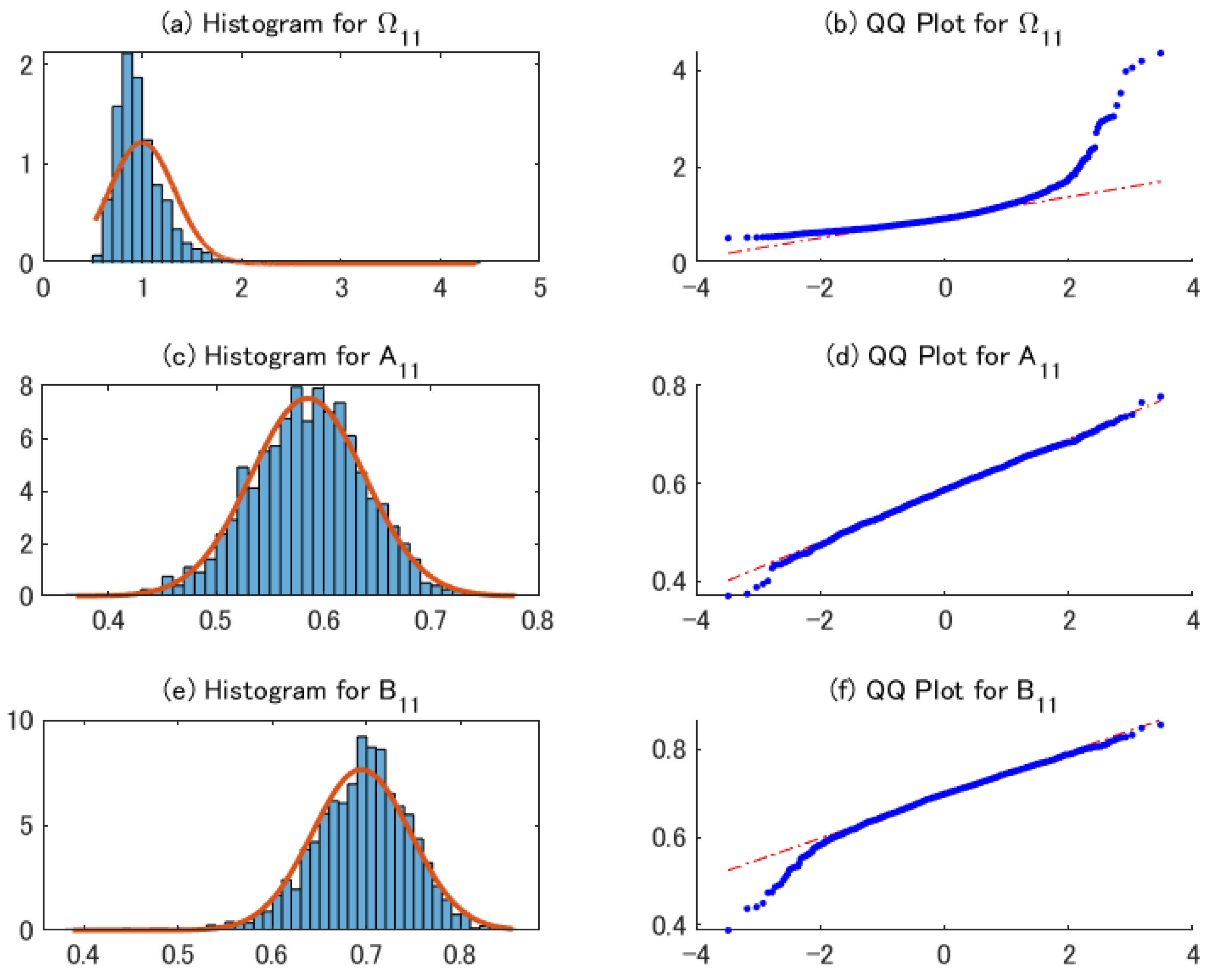
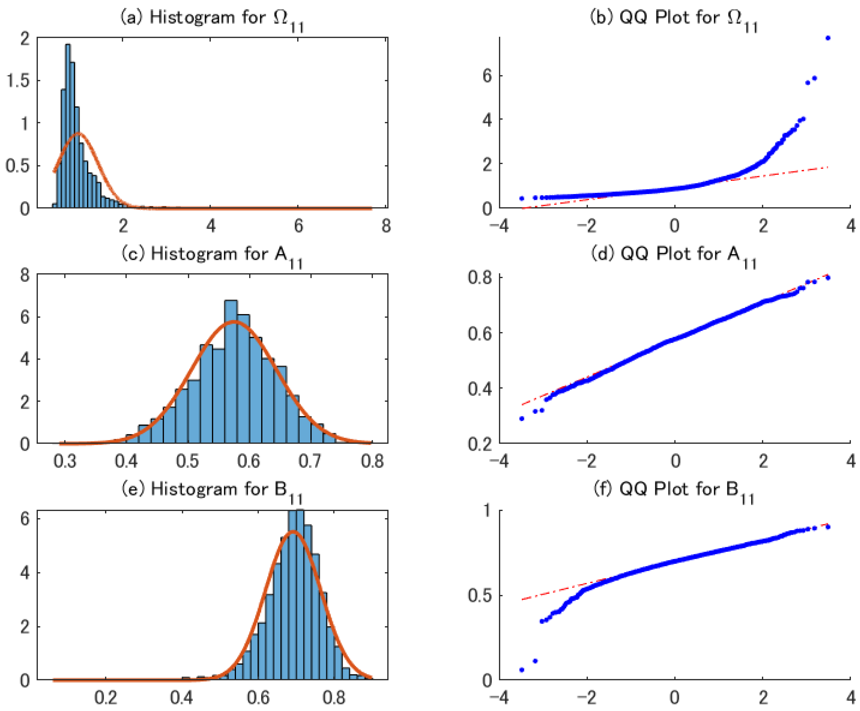
Table 1 shows the sample mean, standard deviations, and root mean squared error of the 2sQML estimates. The table indicates that the bias of the estimators is negligible, even for $T=500$. The standard deviation for the sample covariance matrix is relatively large for DGP1, which is expected to decrease as the sample size increases. Figure 1 shows the histograms and QQ Plots of 2sQML estimates for representative parameters. As the estimate of ${\Omega }_{11}$ is obtained from the sample covariance matrix, its distribution is skewed to the right. By contrast, the distributions of the 2sQML estimates of $A_{11}$ and $B_{11}$ are close to the normal distribution.

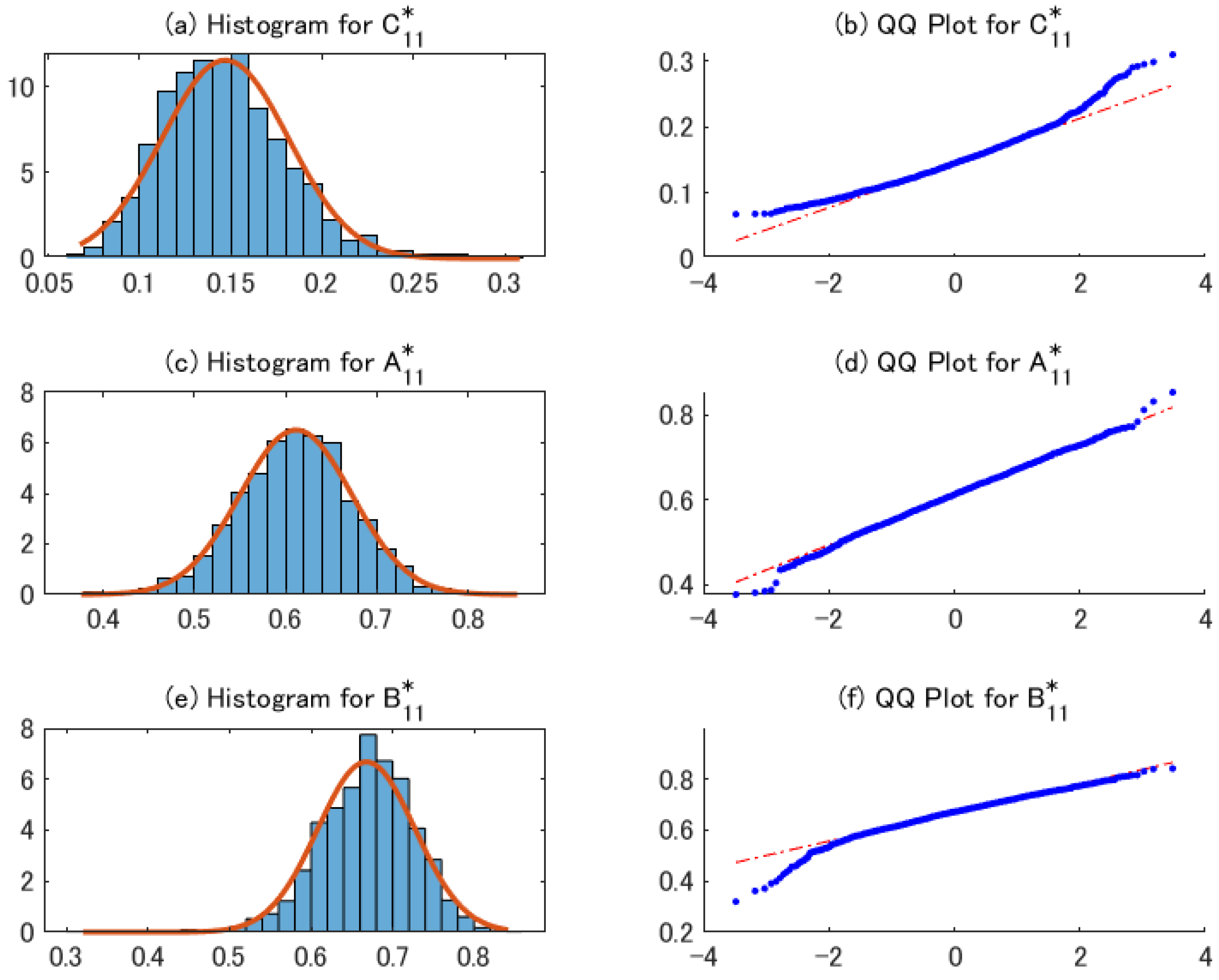
We also check the effects of the transformation from $(\widehat{\Omega },\widehat{A},\widehat{B})$ to $({\widehat{C}}^{*},{\widehat{A}}^{*},{\widehat{B}}^{*})$, as shown in Corollary 1. Table 2 shows the sample mean, standard error, and root mean squared error of the transformed estimator. As in Table 1, the bias of the estimators is negligible. Figure 2 indicates that the transformed estimators for the full BEKK specification can be approximated using the normal distribution.

4.3. Performance of Conditional Covariance Matrix Estimator

In the second experiment, we consider higher-dimensional cases with $d=\{5,10,30\}$. Denoting by $U(a,b)$, we simulate the uniform distribution on $[a,b]$:

$$\begin{array}{cc}\hfill DGP3:& {\Omega }_0={\Xi }_0{\Xi }_0^{\prime },{\Xi }_0=\left(\begin{array}{cccc}{\Xi }_{11,0}& 0& \cdots & 0\\ {\Xi }_{21,0}& {\Xi }_{22,0}& \ddots & 0\\ ⋮& ⋮& \ddots & ⋮\\ {\Xi }_{d1,0}& {\Xi }_{d2,0}& \cdots & {\Xi }_{dd,0}\end{array}\right),\hfill \\ \hfill & A_0=\left(\begin{array}{cccc}{A}_{11,0}& 0& \cdots & 0\\ 0& A_{22,0}& \ddots & 0\\ ⋮& \ddots & \ddots & ⋮\\ 0& 0& \cdots & A_{dd,0}\end{array}\right),B_0=\left(\begin{array}{cccc}{B}_{11,0}& 0& \cdots & 0\\ 0& B_{22,0}& \ddots & 0\\ ⋮& \ddots & \ddots & ⋮\\ 0& 0& \cdots & B_{dd,0}\end{array}\right),\hfill \end{array}$$

where ${\Xi }_{ij,0}\sim U(-0.5,0.5)$$(i\ge j)$, $A_{ii,0}\sim U(0.1,0.4)$, and $B_{ii,0}\sim U(0.85,0.9)$$(i,j=1,2,\dots ,d)$. We discard the parameters which do not satisfy the stationarity condition. Based on the simulated parameters, we generate $X_t$ for the sample size $T=\{500,1000\}$, and estimate the diagonal RBEKK and diagonal BEKK models to calculate the average of the Frobenius norm of the difference in the conditional covariance matrices:

$$\frac{1}{T}\sum _{t=1}^T∥{\widehat{H}}_t-H_{t,0}∥,$$

where ${\widehat{H}}_t$ is the estimated covariance matrix and $H_{t,0}$ is the true covariance matrix. While ${\widehat{H}}_t=H_{t,h}\left(\widehat{\mathit{\theta }}\right)$ for the diagonal BEKK model, ${\widehat{H}}_t$ is similarly defined for the diagonal BEKK model. We use the common random parameters for the two models and repeat the procedure 100 times with different random parameters.

Table 3. Average distance between the true and estimated covariance matrices.

Sample Size	Diagonal RBEKK			Diagonal BEKK
	$\mathit{d}=5$	$\mathit{d}=10$	$\mathit{d}=30$	$\mathit{d}=5$	$\mathit{d}=10$	$\mathit{d}=30$
$\mathit{T}=500$	1.1377	3.9358	41.047	1.5176	6.3447	64.909
$T=1000$	0.7883	2.7948	24.570	1.3800	5.9794	57.433

shows the sample means of the average distances. The values of the measure for $d=10$ are expected to take values approximately four times larger than those for $d=5$, as implied by the dimension of ${\widehat{H}}_t$$(d\times d)$. Table 3 supports this result. As the sample size increases, the average distance decreases. Compared with the diagonal BEKK model, the diagonal RBEKK model has a smaller distance measure.

4.4. Effects of Diagonal Specification

In the third experiment, we examine the effects of the diagonal specification for the BEKK and RBEKK models when the true model is full BEKK. For this purpose, we consider several measures to check the distance from the diagonal BEKK and RBEKK models to the full BEKK model. The non-diagonal indices are defined as:

$$\begin{array}{cc}\hfill & \gamma =∥A^{*}-diag\left(A^{*}\right)∥+∥B^{*}-diag\left(B^{*}\right)∥\left(DiagonalBEKK\right),\hfill \\ \hfill & {\gamma }^r=∥A^{*}-{\Omega }^{1/2}diag\left({\Omega }^{-1/2}{A}^{*}{\Omega }^{1/2}\right){\Omega }^{-1/2}∥+∥B^{*}-{\Omega }^{1/2}diag\left({\Omega }^{-1/2}{B}^{*}{\Omega }^{1/2}\right){\Omega }^{-1/2}∥\hfill \\ \hfill & \left(DiagonalRBEKK\right),\hfill \end{array}$$

(13)

where $diag\left(Y\right)$ creates a diagonal matrix from the square matrix Y. Using the non-diagonal indices, we can calculate the theoretical distance of the diagonal BEKK and RBEKK models. For the remaining measures, we use the estimated values of the parameters of these models. The maximized log-likelihood $L_{T,h}\left(\widehat{\mathit{\theta }}\right)$ is used, as is the average of the Frobenius norm of the difference of the conditional covariance matrices, as explained above.

Using these measures, the following Monte Carlo simulations investigate the effects of the diagonal specification of the BEKK and RBEKK models when the true model is bivariate full BEKK. For this purpose, we consider the specification for (4):

$$A_0^{*}=w{D}_{a1}+(1-w){\Omega }_0^{1/2}{D}_{a2}{\Omega }_0^{-1/2},B_0^{*}=w{D}_{b1}+(1-w){\Omega }_0^{1/2}{D}_{b2}{\Omega }_0^{-1/2},$$

(14)

for $0\le w\le 1$, where $D_{a1}$, $D_{a2}$, $D_{b1}$, and $D_{b2}$ are diagonal matrices. When $w=1$, the specification reduces to the diagonal BEKK model, while it becomes the diagonal RBEKK model for $w=0$. Except for these endpoints, the full BEKK specification provides a non-diagonal structure for $A_0^{*}$ and $B_0^{*}$ in (4) and $A_0$ and $B_0$ in (5). For the specification in (4), the non-diagonal indices provide the linear functions of w:

$${\gamma }_w=\xi (1-w),{\gamma }_w^r={\xi }_{r}w,$$

where

$$\begin{array}{cc}& \xi =∥{\Omega }_0^{1/2}{D}_{a2}{\Omega }_0^{-1/2}-diag\left({\Omega }_0^{1/2}{D}_{a2}{\Omega }_0^{-1/2}\right)∥+∥{\Omega }_0^{1/2}{D}_{b2}{\Omega }_0^{-1/2}-diag\left({\Omega }_0^{1/2}{D}_{b2}{\Omega }_0^{-1/2}\right)∥,\hfill \\ & {\xi }_r=∥D_{a1}-{\Omega }_0^{1/2}diag\left({\Omega }_0^{-1/2}{D}_{a1}{\Omega }_0^{1/2}\right){\Omega }_0^{-1/2}∥+∥D_{b1}-{\Omega }_0^{1/2}diag\left({\Omega }_0^{-1/2}{D}_{b1}{\Omega }_0^{1/2}\right){\Omega }_0^{-1/2}∥,\hfill \end{array}$$

to calculate the theoretical distances. Consider the parameter settings for the DGPs as:

$$\begin{array}{cc}& {DGP4}_w:({\Omega }_0,A_0,B_0)inDGP1,with{D}_{a1}=D_{a2}=A_{0}and{D}_{b1}=D_{b2}=B_{0}in\left(\right),\hfill \\ & {DGP5}_w:({\Omega }_0,A_0,B_0)inDGP2,with{D}_{a1}=D_{a2}=A_{0}and{D}_{b1}=D_{b2}=B_{0}in\left(\right).\hfill \end{array}$$

Set $w=0,0.1,\dots ,1$ to examine 11 cases, with $T=500$ and the number of replications set to 100. We estimate the diagonal RBEKK model using the 2sQML method, while VT-QML is used for the diagonal BEKK model.

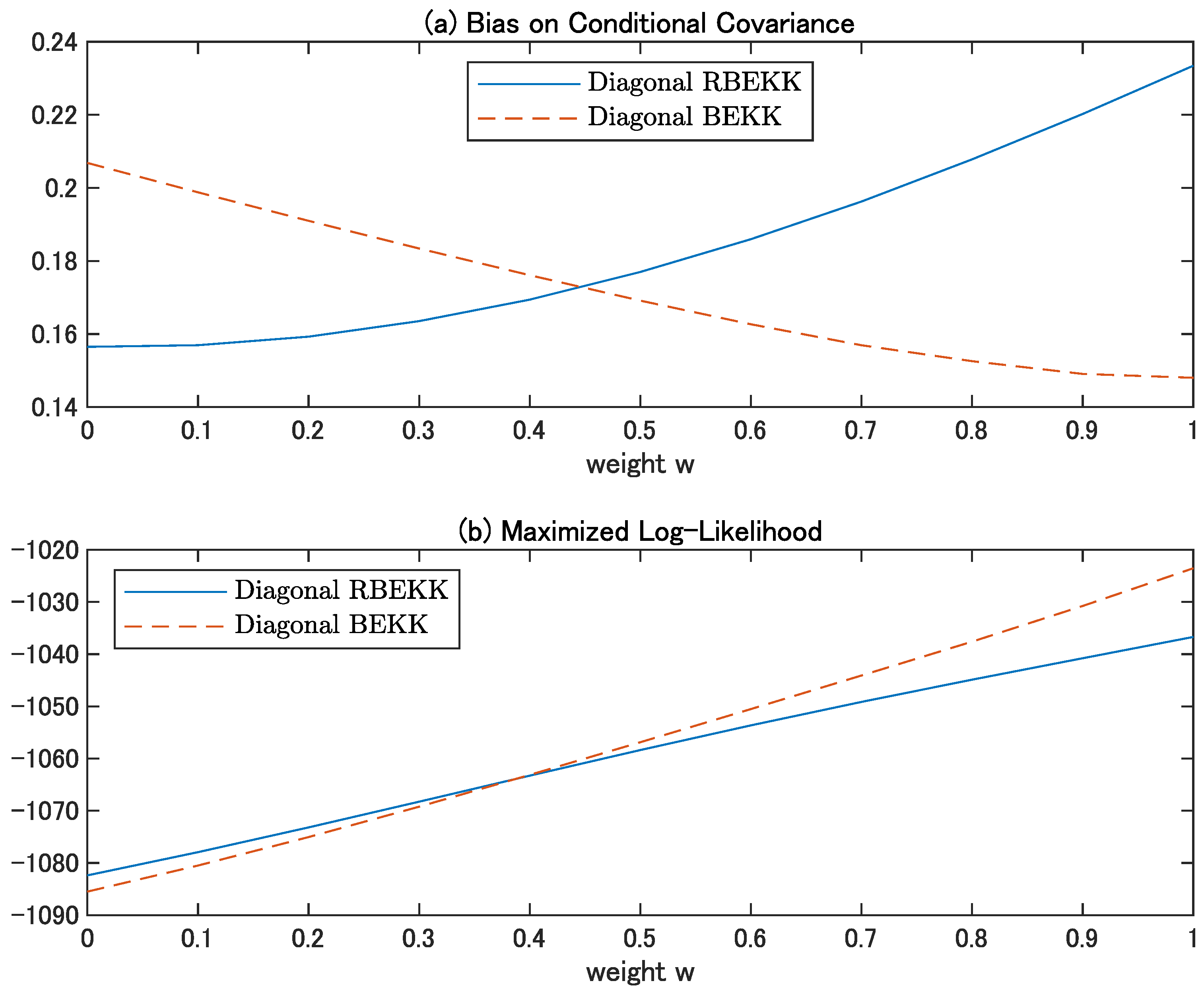
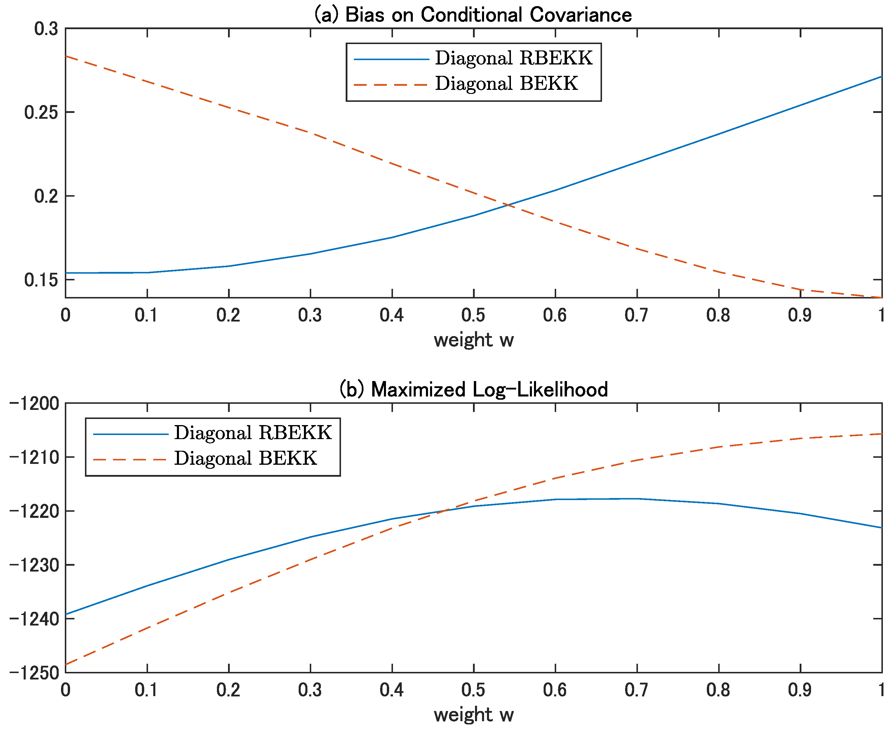
Figure 3 and Figure 4 show the sample means of the average bias for the conditional covariance matrices and sample means of the maximized log-likelihood function for DGP3 and DGP4, respectively. As expected from the structure, the superiority of the diagonal models depends on the structure of the true BEKK model. If w is closer to zero, the diagonal RBEKK model is preferred. The non-diagonality indices are

$$\begin{array}{cc}& {DGP4}_w:{\gamma }_w=0.0212(1-w),{\gamma }_w^r=0.0309w,crossingat{w}^{†}=0.407,\hfill \\ & {DGP5}_w:{\gamma }_w=0.0563(1-w),{\gamma }_w^r=0.0614w,crossingat{w}^{†}=0.479,\hfill \end{array}$$

and these theoretical values of $w^{†}$ correspond to the intersections shown in Figure 3b and Figure 4b, respectively. The Akaike information criterion and Bayesian information criterion lead to the same conclusion, as the numbers of parameters in these two models are the same.

4.5. Heavy Tails and Moment Conditions

The last experiment uses DGPs 1 and 2 with the multivariate standardized t distribution and the degree-of-freedom parameter $\nu$ (denoted by $St\left(\nu \right)$), instead of the multivariate standard normal distribution. We consider three cases: (i) a heavy-tailed distribution ($\nu =7$), which satisfies Assumption 4(a); (ii) DGPs in which the sixth moments are not finite ($\nu =5$); and (iii) DGPs in which the fourth moments are not finite ($\nu =5$). The latter two cases imply that the 2sQML estimator is consistent, but its asymptotic normality is not guaranteed. As an alternative approach, we may use the parameter condition derived from Theorem 3 of Hafner (2003). To save space, we omitted the tables for the sample mean, standard deviations, and root mean squared error of the 2sQML estimates, which are available in the Supplementary Materials.

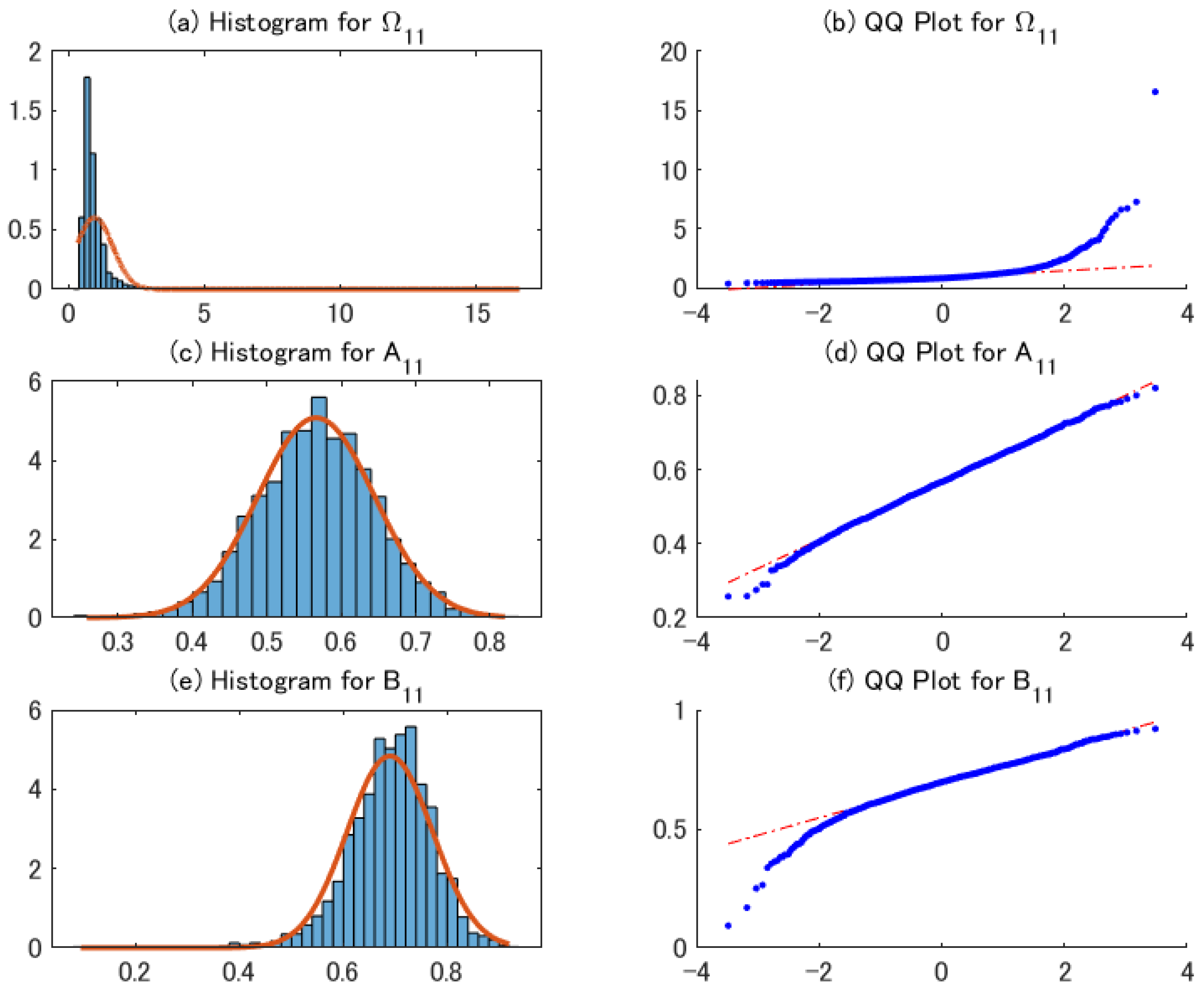
Figure 5 shows the histograms and QQ plots of 2sQML estimates for DGP1 with $St\left(7\right)$. The Monte Carlo results indicate that the bias is negligible, and the standard deviations are larger than in the case of standard normal distribution. The distributions of the estimates of ${\Omega }_{11}$, $A_{11}$, and $B_{11}$ are similar to those of Figure 1. This result supports Proposition 2.

Figure 6 shows the histograms and QQ plots of 2sQML estimates for DGP1 with $St\left(5\right)$. Although the sixth moments are not finite, the distributions of the estimates of ${\Omega }_{11}$, $A_{11}$, and $B_{11}$ are close to those of Figure 5. This result implies that we can relax Assumption 4 to guarantee asymptotic normality for the second-step estimator.

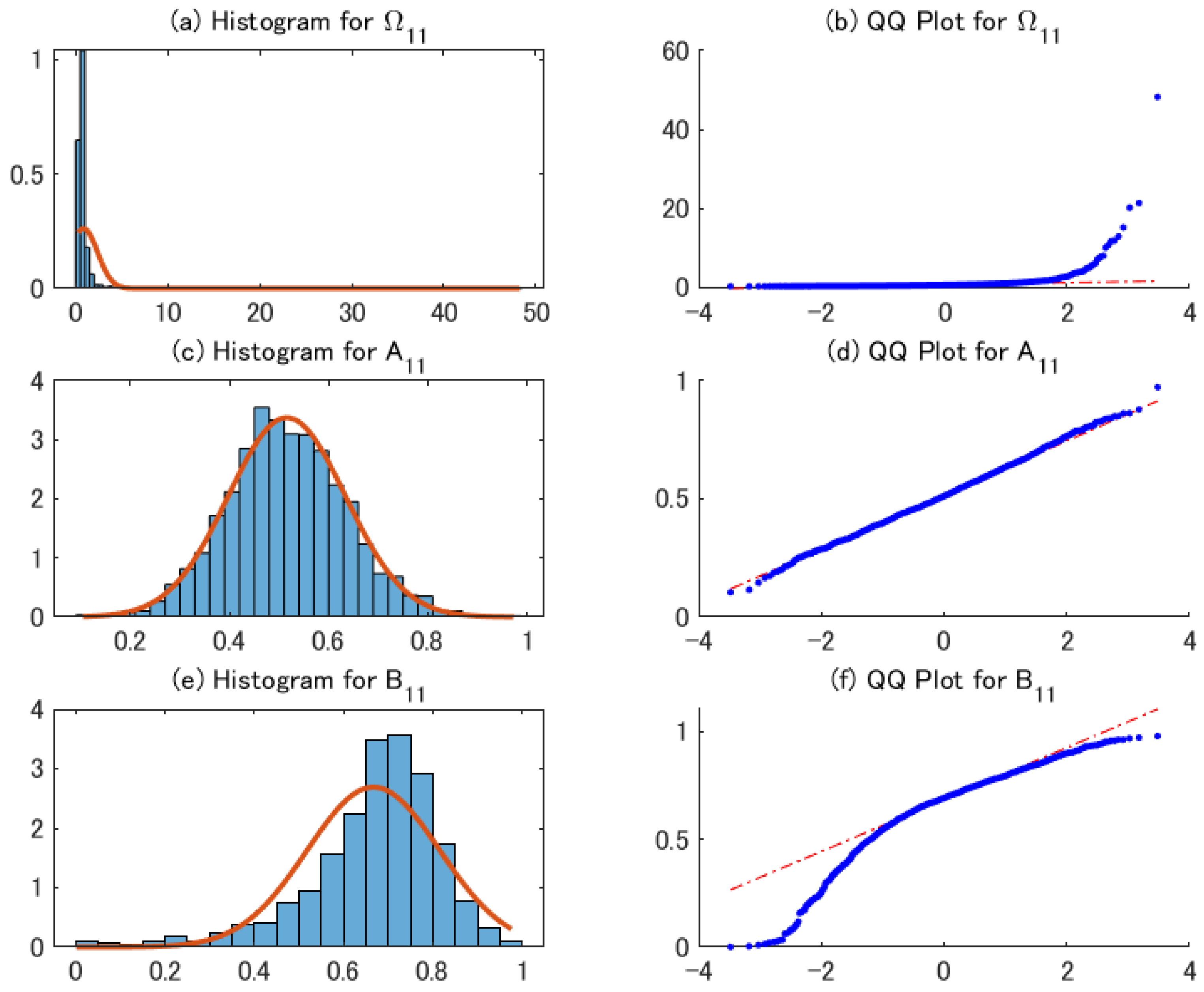
For the DGPs with $St\left(3\right)$, the Monte Carlo result shown in the Supplementary Materials indicates that the bias of the estimators for $\Omega$ and A are relatively small, compared with those of $B_{11}$ and $B_{22}$. Figure 7 shows the histograms and QQ plots of 2sQML estimates for DGP1 with $St\left(5\right)$. The QQ plot of Figure 7a shows the instability of the first-step estimator. The instability affects the standard deviations of the second-step estimator. Figure 7e implies that the effects are more serious on the estimates of $B_{11}$, with a pressure towards zero. The result indicates that a larger sample size is required in order to improve the estimates for the parameters of B.

The Monte Carlo experiments show that the finite sample properties of the 2sQML estimator are satisfactory and that the average distance between the true and estimated covariance matrices indicates that the difference between the two diagonal BEKK models is not negligible. Because it is difficult to estimate the fully parametrized BEKK model for higher d, it is necessary to examine the model specifications, as in Noureldin et al. (2014), using parsimonious specifications. The Monte Carlo experiments indicate that we may relax the assumption for the sixth moments for the second step estimator.

5. Empirical Analysis

In this section, we assess the diagonal specification of the RBEKK model compared with the diagonal BEKK model. For this purpose, we focus on the out-of-sample forecasts evaluation, adopting the approach of Engle and Colacito (2006), for the mean-variance portfolio. We calculate the returns of stocks listed on the Dow Jones Industrial Average, except for Dow Inc. ($d=29$), for the period starting from 18 February 2010 to 23 January 2020, yielding 2500 observations. We exclude Dow Inc. since it went public on April 1, 2019. Fixing the sample size as $T=2000$, we use rolling windows to obtain one-step-ahead forecasts for the last 500 observations for model i$(i=1,2)$, denoted by ${\widehat{H}}_t^{\left(i\right)}$$(t=2001,\dots ,2500)$. While Model 1 is the diagonal RBEKK model, Model 2 is the diagonal BEKK.

For our portfolio analysis, we consider the minimum variance portfolio, which gives the weight vector for model i chosen at the end of time $t-1$, ${\mathbf{w}}_{it}={\widehat{H}}_t^{\left(i\right)-1}\iota /\left({\iota }^{\prime }{\widehat{H}}_t^{\left(i\right)-1}\iota \right)$, where $\iota$ is the $d\times 1$ vector of ones. Engle and Colacito (2006) show that the realized portfolio volatility is the smallest one when the variance-covariance matrices are correctly specified. We define the distance based on the difference of the squared returns of the two portfolios as:

$$e_t={\left\{{\mathbf{w}}_{1t}^{\prime }{X}_t\right\}}^2-{\left\{{\mathbf{w}}_{2t}^{\prime }{X}_t\right\}}^2.$$

(15)

Since the portfolio variances are the same if the forecasts of the covariance matrices are the same, we examine the null hypothesis $H_0:$$E\left(e_t\right)=0$ using the Diebold and Mariano (1995) test. In this case, the test can be constructed in the following manner. Consider the linear regression model given by $e_t={\mu }_e+u_{et}$ with $E\left(u_{et}\right)=0$, and test $H_0:$${\mu }_e=0$ using the heteroskedasticity- and autocorrelation-consistent standard errors. If the mean of $e_t$ is negative (positive), the diagonal RBEKK (the diagonal BEKK) model is preferred.

Table 4. Engle and Colacito (2006) test.

Parameter	Estimate	HAC S.E.	t-Value
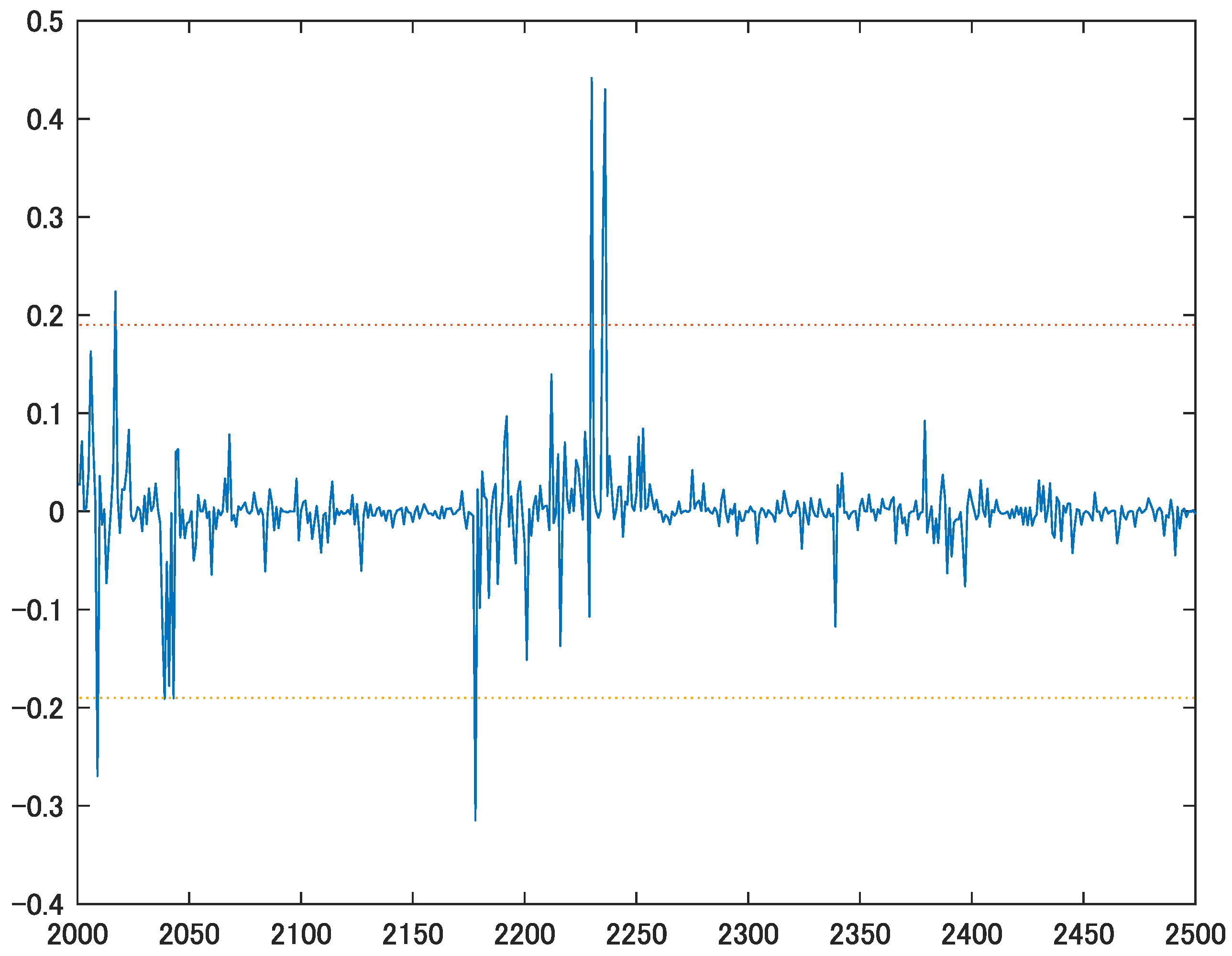
${\mu }_e$	0.0010	0.0043	0.2192

indicates that the Engle and Colacito (2006) test fails to reject the null hypothesis that the two forecasts are equivalent. Figure 8 shows the difference of squared portfolio returns, defined by Equation (15), accompanied by the 95% confidence interval. With a few exceptions, there is no significant difference between the two portfolio weights calculated by the forecasts of the two different models. For instance, at time $t=2178$, the forecast by the diagonal RBEKK is preferred. As discussed in Section 4.4, the choice of the diagonal RBEKK or the diagonal BEKK model depends on the true structure of the full BEKK. Figure 8 supports the result of the Engle and Colacito (2006) test in Table 4. To improve the forecasting performance, we may consider a more general rotation matrix, as in Asai and McAleer (2020) and Hafner et al. (2020).

6. Conclusions

For the RBEKK-GARCH model, we show the consistency and asymptotic normality of the 2sQML estimator under weak conditions. The 2sQML estimation uses the unconditional covariance matrix for the first step and rotates the observed vector to have the identity matrix for its sample covariance matrix. The second step conducts the QML estimation for the remaining parameters. While we require second-order moments for consistency because of the estimation of the covariance matrix, we need finite sixth-order moments for asymptotic normality, as in Pedersen and Rahbek (2014). We also show the asymptotic relation of the 2sQML estimator for the RBEKK model and the VT-QML estimator for the VT-BEKK model. The Monte Carlo results show that the finite sample properties of the 2sQML estimator are satisfactory, and that the adequacy of the diagonal RBEKK depends on the structure of the true parameters. The empirical result for the returns of stocks listed on the DOW30 indicates that the diagonal RBEKK and diagonal BEKK models are competitive, with the superiority of each model changing over time.

As an extension of the dynamic conditional correlation (DCC) model of Engle (2002), Noureldin et al. (2014) suggested rotated DCC models (for a caveat about the regularity conditions underlying DCC, see McAleer (2018)). We can apply the rotation to the different kinds of correlation models suggested by McAleer et al. (2008) and Tse and Tsui (2002). Together with such extensions, the derivation of asymptotic theory for the rotated DCC models is an important direction for future research.

References

- Alexander, Carol, ed. 2001. Orthogonal GARCH. In Mastering Risk. Hoboken: Financial Times-Prentice Hall, pp. 21–28. [Google Scholar]
- Asai, Manabu, and Michael McAleer. 2020. Multivariate Hyper-Rotated GARCH-BEKK: Asymptotic Theory and Practice. Tokyo: Soka University, Unpublished Paper. [Google Scholar]
- Baba, Yoshihisa, Robert. F. Engle, Dennis Kraft, and Kenneth F. Kroner. 1985. Multivariate Simultaneous Generalized ARCH. San Diego: University of California, Unpublished Paper. [Google Scholar]
- Bauwens, Luc, Sébastian Laurent, and Jeroen K. V. Rombouts. 2006. Multivariate GARCH models: A survey. Journal of Applied Econometrics 21: 79–109. [Google Scholar] [CrossRef] [Green Version]
- Bollerslev, Tim. 1986. Generalized autoregressive conditional heteroskedasticity. Journal of Econometrics 31: 307–27. [Google Scholar] [CrossRef] [Green Version]
- Boussama, Farid, Florian Fuchs, and Robert Stelzer. 2011. Stationarity and geometric ergodicity of BEKK multivariate GARCH models. Stochastic Processes and Their Applications 121: 2331–60. [Google Scholar] [CrossRef] [Green Version]
- Chang, Chia-Lin, and Michael McAleer. 2019. The fiction of full BEKK: Pricing fossil fuels and carbon emissions. Finance Research Letters 28: 11–19. [Google Scholar] [CrossRef]
- Comte, Fabienne, and Offer Lieberman. 2003. Asymptotic theory for multivariate GARCH processes. Journal of Multivariate Analysis 84: 61–84. [Google Scholar] [CrossRef] [Green Version]
- Diebold, Francis X., and Roberto S. Mariano. 1995. Comparing predictive accuracy. Journal of Business & Economic Statistics 13: 253–63. [Google Scholar]
- Engle, Robert F. 1982. Autoregressive conditional heteroskedasticity with estimates of the variance of United Kingdom inflation. Econometrica 50: 987–1007. [Google Scholar] [CrossRef]
- Engle, Robert F. 2002. Dynamic conditional correlation: A simple class of multivariate generalized autoregressive conditional heteroskedasticity models. Journal of Business & Economic Statistics 20: 339–50. [Google Scholar]
- Engle, Robert F., and Kenneth F. Kroner. 1995. Multivariate simultaneous generalized ARCH. Econometric Theory 11: 122–50. [Google Scholar] [CrossRef]
- Engle, Robert F., and Riccardo Colacito. 2006. Testing and valuing dynamic correlations for asset allocation. Journal of Business & Economic Statistics 24: 238–53. [Google Scholar]
- Francq, Christian, Lajos Horváth, and Jean-Michel Zakoïan. 2011. Merits and drawbacks of variance targeting in GARCH models. Journal of Financial Econometrics 9: 619–56. [Google Scholar] [CrossRef] [Green Version]
- Hafner, Christian M. 2003. Fourth moment structure of multivariate GARCH models. Journal of Financial Econometrics 1: 26–54. [Google Scholar] [CrossRef]
- Hafner, Christian M., Helmut Herwartz, and Simone Maxand. 2020. Identification of structural multivariate GARCH models. Journal of Econometrics. [Google Scholar] [CrossRef]
- Hafner, Christian M., and Arie Preminger. 2009. On asymptotic theory for multivariate GARCH models. Journal of Multivariate Analysis 100: 2044–54. [Google Scholar] [CrossRef] [Green Version]
- Lanne, Markku, and Pentti Saikkonen. 2007. A multivariate generalized orthogonal factor GARCH model. Journal of Business & Economic Statistics 25: 61–75. [Google Scholar]
- Laurent, Sébastian, Jeroen V. K. Rombouts, and Francesco Violante. 2012. On the forecasting accuracy of multivariate GARCH models. Journal of Applied Econometrics 27: 934–55. [Google Scholar] [CrossRef] [Green Version]
- Lütkepohl, Helmut. 1996. Handbook of Matrices. New York: John Wiley & Sons. [Google Scholar]
- McAleer, Michael. 2005. Automated inference and learning in modeling financial volatility. Econometric Theory 21: 232–61. [Google Scholar] [CrossRef] [Green Version]
- McAleer, Michael. 2018. Stationarity and invertibility of a dynamic correlation matrix. Kybernetika 54: 363–74. [Google Scholar] [CrossRef] [Green Version]
- McAleer, Michael, Felix Chan, Suhejla Hoti, and Offer Lieberman. 2008. Generalized autoregressive conditional correlation. Econometric Theory 24: 1554–83. [Google Scholar] [CrossRef] [Green Version]
- Noureldin, Diaa, Neil Shephard, and Kevin Sheppard. 2014. Multivariate rotated ARCH models. Journal of Econometrics 179: 16–30. [Google Scholar] [CrossRef] [Green Version]
- Pedersen, Rasmus S., and Anders Rahbek. 2014. Multivariate variance targeting in the BEKK-GARCH model. Econometrics Journal 17: 24–55. [Google Scholar] [CrossRef] [Green Version]
- Silvennoinen, Annastiina, and Timo Teräsvirta. 2009. Multivariate GARCH models. In Handbook of Financial Time Series. Edited by Toben G. Andersen, Richard A. Davis, Jens-Peter Kreiss and Thomas Mikosch. New York: Springer, pp. 201–29. [Google Scholar]
- Tse, Y. K., and Albert K. C. Tsui. 2002. A multivariate generalized autoregressive conditional heteroscedasticity model with time-varying correlations. Journal of Business & Economic Statistics 20: 351–61. [Google Scholar]
- van der Weide, Roy. 2020. GO-GARCH: A multivariate generalized orthogonal GARCH model. Journal of Applied Econometrics 17: 549–64. [Google Scholar] [CrossRef]
Figure 1.
Histograms and QQ plots of 2sQML estimates for DGP1.
Figure 2.
Histograms and QQ plots of 2sQML estimates for DGP1 with full BEKK parameters.
Figure 3.
Comparison of the diagonal specifications for the BEKK and RBEKK models: DGP4.
Figure 4.
Comparison of the diagonal specifications for the BEKK and RBEKK models: DGP5.
Figure 5.
Histograms and QQ plots of 2sQML estimates for DGP1 with .
Figure 6.
Figure 7.
Figure 8.
Difference of squared portfolio returns. Note: The solid line shows the value of , defined by Equation (15), while the dotted lines indicate the confidence interval.